POLICY INERTIA OR POLICY LEARNING? AGOSTINO CONSOLO* Abstract. The literature on monetary policy commonly characterizes the policy behavior as cautious by admitting a partial adjustment of the policy rate with respect to economic conditions. Theoretical frameworks as those proposed by Rudebusch (2002) and Soderlind et al. (2005) show that such a gradualism implies high predictability of interest rates. Specularly, the nance literature looks at term structure evidence and shows that interest-rates predictability is low at horizons greater than two quarters. Even though policy gradualism is, to some extent, a very convincing argument from several theoretical perspectives, the degree of inertia provided by the macro view is too high to be consistent with the term structure evidence. This paper is an attempt to reconcile the failure of such macro models in modelling interest rates. We depart from the rational expectations paradigm and, in contrast, we adopt a learning approach to describe the equilibrium of the economy. After solving the model, we
nd that (a) the degree of partial adjustment may
derive from misspeci cation errors caused by not considering the learning behavior of policymaking, (b) the model implies lower predictability of interest rates, (c) the learning process of the Monetary Authority has an important dynamic.
1. Introduction There is a growing literature in macroeconomics which is relaxing the core assumption of rational expectations to focus on a di erent mechanism of expectations formation. In fact, agents are not endowed with common knowledge of the economy and their information schemes can be asymmetric given the state of the economy. Therefore, in general, Date: September 9, 2005. Key words and phrases. Monetary Policy, Learning, Time-Varying Parameters Models. *Bocconi University. [Sept 9th, 2005]. Preliminary Version.
[email protected]. I am grateful to Fabio Canova, Carlo Favero and Ulf Soderstrom for helpful comments. All errors are my own responsibility. 1
2
AGOSTINO CONSOLO
agents either don't know the parameters in the model's economy or the model itself can be misspeci ed. Limited information is examined by assuming that agents adopt a learning algorithm to recover deep parameters as new information becomes available. Proceeding in this way, they can eventually converge to a rational expectations equilibrium (REE). On the other hand, omitting an important part of the model's speci cation leads to a case of self-con rming equilibrium: they may never converge to the REE. By considering the adaptive learning mechanism, we let agents form expectations according to their perceived law of motion (PLM), which needs to be estimated conditional on the available information. We also assume that agents' PLM is not misspeci ed so that self-con rming equilibria are ruled out. The economy studied in this paper models both private agents and central bank's expectations allowing for some degree of discrepancy between their information sets. In particular, we assume that the central bank cannot measure some deep parameters of the models while (homogenous) private agents don't have full observability of monetary policy. While private agents need to form expectations with respect to the output gap and the in ation rate, the central bank has to recover structural parameters taking private expectations as given. As far as the transmission mechanism is concerned, whenever the monetary policy authority modi es its policy rate or its belief regarding deep parameters, this will induce changes in in ation and in the output gap. This will feed back to new estimated structural parameters and in turn it will a ect private expectations. Under the E-Stability Principle, this process will converge to the REE. In this environment feedbacks matter a lot because of inconsistency of expectations and, conditional on the learning algorithm, they a ect the adjustment process to the REE. The present work looks at simple monetary policy rules. In particular, we will mainly concentrate on instruments-based rules a' la Taylor (1993) and a' la Clarida et al. (2000) to tackle the current debate on monetary policy inertia, but di erently to what has been done until now, we introduce uncertainty on model parameters. Monetary policy inertia
LEARNING AND MONETARY POLICY RULES
3
or interest rate smoothing is de ned as a partial adjustment of the money market e ective interest rate with respect to the optimal rate deriving from a behavioral rule. Such form of policy gradualism has found both theoretical and empirical support which conveys that central banks around the world do not respond quickly to shocks to the economy. Anyhow, if central banks aim to learn about the structural model, policy inertia as de ned above no longer holds even though the policy rate still follows a gradual adjustment path.
1.1. Theoretical and Empirical Literature. The theoretical literature has derived insightful motivations about why central banks want to smooth interest rates in conducting monetary policy. According to Woodford (2002), if the monetary authority targets the in ation rate, the output and interest-rate gaps and commits to an optimal rule, then partial adjustment naturally arises and it can be justi ed by the fact that under commitment central banks are able to in uence future private expectations1. Alternatively, under discretion, by appropriately modifying the central bank's loss function2 Woodford (2002) provides justi cation for the partial adjustment argument. Such a policy gradualism is optimal in the sense that it can help to reduce output and in ation volatility. Clarida et al. (2000) also support a high degree of policy inertia by estimating an expectations-based policy rule. Moreover, they nd that such a policy rule is stabilizing for the economy they are considering: such a result is crucially a ected by the sluggishness of the interest-rate adjustment3. Furthermore, as discussed in Sack and Wieland (1999), other plausible explanations justify the reason why a central bank could optimally choose to gradually adjust the policy rate which may not be consistent with the partial adjustment story. Their work concentrates on the forward-looking behavior of market participants, data uncertainty 1
CB can a ect the economy only if it is able to modify long interest rates. Being able to determine the future path of private expectations is something which is truly desiderable from its point of view. 2 Such a modi cation in the loss function is justi ed by an "optimal delegation" argument. 3 They are mainly focused on the in ation's coe cient: Values larger or smaller than one have di erent e ects on the real interest rate and on the economy as a whole.
4
AGOSTINO CONSOLO
and parameters uncertainty. Indeed, they support interest-rate smoothing without referring to a monetary policy objective function. By considering forward-looking expectations, small policy changes (without reversals) are su cient to stabilize the economy because private agents' expectations are a ected by such policies and not only do variables react by the amount of policy changes but also to variations in private agents' behavior.4 As far as data uncertainty is concerned, Orphanides (1998) points out that by letting the monetary authority adjust interest rates with upcoming information and by considering possible measurement errors we get a closer picture of what we observe in practice. Orphanides' conclusion is the decrease in policymaking responsiveness to new data for output gap and in ation, but he doesn't show that a high degree of partial adjustment is needed. Parameters uncertainty is seen as another justi cation for monetary policy inertia. According to Sack and Wieland (1999), by appropriately taking parameters uncertainty into account we observe a reduction in the volatility of the policy rates. However, there could be circumstances in which parameters uncertainty may induce the policymaker to behave more aggressively.5 Conversely, there is an emerging macro- nance literature which aims at match empirical facts deriving both from the term structure of interest rates and from macro models analyzed by means of monetary policy rules. An example is Rudebusch (2002) who shows that an inertial policy rule is observational equivalent to a policy rule with no partial adjustment and persistent shocks. That means central banks are not smoothly adjusting the policy rate, but they are just responding to persistent factors in the economy.6 4
It was shown by Levin et al. (1998) that for a given level of interest-rate volatility, a gradual rule can reach a better policy frontier. 5 Experimentation is one of the cases in which the monetary authority wants to learn the e ect of a large policy movement. Another case is the one analyzed by Soderstrom (2000) who uses a small macro model with an optimizing monetary authority facing parameters uncertainty. He nds that whenever the policymaker is uncertain about the persistence of in ation, the optimal rule suggest to react more aggressively to dampen future uncertainty. 6 In contrast to Rudebusch's analysis, English et al. (2003) implement a testing procedure between the partial adjustment model and a serially-correlated-error speci cation. They are able to reason that the
LEARNING AND MONETARY POLICY RULES
5
The seminal paper of Taylor (1993) suggested a simple rule to describe monetary policy in practice, which was supposed to hold as a common run. Therefore, deviations from such a rule have to be considered as occasional episodes. However, residuals from estimating the Taylor's original speci cation are highly serially correlated which suggests misspeci cation problems. One solution to this problem can be found by recalling the theoretical and empirical literature based on interest-rate smoothing motives which justi es the introduction of a lagged interest rate in the policy rule that cleans out the residuals from their persistence. This way of proceeding is not commonly well accepted because it represents more a statistical artifact than an economic patch. As a matter of fact, Griliches (1961) and Hendry (1978) conclude that it is not infrequent in time series econometrics to estimate a dynamic equation with a high and signi cant distributed lag coe cients (that justi es the partial adjustment story). Griliches (1961) nds that a "signi cant coe cient for the lagged dependent variable is likely to be positive even though the true coe cient is zero, as long as the serial correlation in the residuals is positive". Similarly, Hendry (1978) a rms that assuming serially correlated errors is not an innocuous assumption, but a convenient simpli cation to approximate (statistically) the misspeci cation error of the estimated model. The case for omitted variables was worked out by assuming a wider information set at the central bank's disposal. A lot of work to this respect is done by studying factors models that re ect the large amount of information central banks have. However, crucial information for monetary policy decisions is not worked out in the same way over time, latter is not supported by the data because actual interest rates changes don't move one-to-one with policy rate changes. This fact discriminate between these two speci cations. Furthermore, they build up an encompassed model including both characteristics and conclude that both the degree of partial adjustment and serial correlation are relevant even though the former is the more important factor in accounting for the deviations from a non-inertial policy rule. English et al. (2003) analysis is based on re-writing the model in rst-di erences and on running hypothesis testing on the coe cients of the two speci cations. Osterholm and Welz (2005) show, by running a simulation excercise, that the type of hypothesis testing performed by English et al. (2003) is not robust, especially in the case of misspeci cation. They work out a standard small-scale NewKeynesian macro model to point out that the possible source of autocorrelated residuals derives from an omitted variables problem.
6
AGOSTINO CONSOLO
that is, there is no constant mechanism which reveals what the more important shock for in ation and output is. Such a state-dependent structure implies that wider-informationsets policy rules can still justify a relevant degree of policy inertia as it happens to be. The approach followed in this work, instead, will focus on a learning mechanism of the agents in the economy. We will start by relaxing the assumption of complete information by assuming that the policymaker doesn't know the structural parameters of the economy and private agents don't observe policy expectations. The learning process is set to recover such unknown measures by the agents. The overall setup is a departure from the RE framework where parameters are assumed to be known a priori (because they were somehow calibrated or estimated) and they are not a ected by any new information contained in the data.
The learning framework, instead, is based on the fact that not only do parameters a ect data, but data can in uence parameters as well. Such non-separability between data and parameters was introduced in the analysis of monetary policy by Wieland (1998). Here, we want to stress that monetary policy rather than partially adjusting the interest rate target, it accommodates the interest rate by slightly modifying the measure of the policy parameters as soon as new information about the in ation rate and the output gap is available. The reduced-form speci cation turns out to have a richer feedback dynamics: this has two consequences. The rst one has to do with the source of misspeci cation of the policy rule, while the second one refers to the fact that policy behavior hasn't had a two regime period as supposed by (Clarida et al. (2000)), but it is more consistent with a ne-tuning procedure over the business cycle.
The remainder of the paper is as follows. Section 2 presents a standard small macro model used in the literature for monetary policy analysis and solves for its rational expectations equilibrium which will represent the benchmark scenario for the rest of the analysis. Successively, in Section 3, the learning approach is introduced and the agents'
LEARNING AND MONETARY POLICY RULES
7
perceived law of motion is constructed. The model under learning is thus solved and once the ALM is recovered, the most important results in terms of forecastability of interest rates and misspeci cation of the common framework based on Taylor-type rules are shown. In section 4, the reduced-form version of the model is taken to the data. In particular, a time-varying coe cient Taylor-type rule is estimated and evaluated showing some asymmetries in the monetary policy behavior in treating recessions and expansion phases. Section 5 discusses the model with respect to the current literature and section 6 concludes.
8
AGOSTINO CONSOLO
2. A Model Economy and The REE The economic environment we present is a stylized version of an optimizing model. Households' behavior is modelled following McCallum and Nelson (1998) and Fuhrer (1998): the utility function is characterized by external habit formation, which is not time separable in consumption. There are two storage technologies which are represented by real money balances and government bonds. The Euler equation derived from the households' problem looks like (2.2), but we have simpli ed the notation for coe cients. We also assume that nal goods are produced by making use of intermediate di erentiated goods according to a Dixit-Stiglitz technology. Therefore, intermediate rms have monopolistic power and they optimally set prices following the Calvo's scheme. We allow the remaining of part of non-optimizing rms to determine prices according to indexation to the previous price level. The log-linearized version of the Euler equation for rms produces the Phillips curve in (2.1). Alternatively, we could have obtained a similar characterization of the Phillips curve by relaxing the assumption of monopolistic competition and allowing for overlapping wage contracts a' la Fuhrer and Moore (1995). The anonymous labels for these coefcients favors both interpretations: however, these coe cients have to be thought as nonlinear functions of deep parameters. The typical source of uncertainty in this kind of models is governed by two types of shocks (ut ; vt ): the former is a cost-push shock which triggers the policy trade-o , while the latter represents an aggregate demand shock (2.1) (2.2)
t
=
xt =
k L Et
t+1
+
k B t 1
e L Et xt+1
+
e B xt 1
+ xt + ut ; (it
Et
t+1 )
+ vt :
Moreover, the central bank reaction function is depicted as an instrument-based rule a' la Clarida et al. (2000) which is the forward-looking version of the one originally proposed by Taylor (1993). Equation (2.3) also recalls the adjustment speci cation by taking
into account: only (1
) of the target rate is considered. It also needs to be
LEARNING AND MONETARY POLICY RULES
9
noticed that "t represents the non-systematic part of monetary policy:7 (2.3)
it = (1
)(
Et
t+1
+
x Et xt+1 )
+ it
1
+ "t :
In this section we brie y describe the REE because we are interested in comparing this model solution to the one that will be recovered in the next section under learning. According to the RE paradigm, expectations are model consistent and agents, both private agents and central bank, have complete knowledge of the model which leads to assume that Et ( ) is a good measure for both: To nd out the equilibrium law of motion in this framework we numerically solve the system of three equations (2.1)-(2.3) by employing the method of undertermined coe cients. In matrix notation, it reads 2
1 0 6 6 6 0 1 0 4 0 0 1
32
3
2
32
k L
3
E 0 0 76 t 7 7 6 t t+1 7 6 76 7 6 7 7 6 e 7 6 xt 7 = 6 (1 6 E x 7+ ) x 0 7 L 54 5 4 t t+1 5 5 4 (1 ) (1 ) x 0 it Et it+1 32 2 3 2 32 3 k 0 0 1 0 0 u t 1 t 76 6 B 7 6 76 7 76 6 7 6 76 7 e +6 0 + 7 6 7 6 7 6 7; 0 x 0 1 0 v t 1 t B 54 4 5 4 54 5 0 0 it 1 0 0 1 "t
which can be written more compactly as (2.4)
Gyt = F Et yt+1 + Hyt
1
+ M et :
The REE is the set fP ; Q g which solves the following xed-point problem (2.5)
Q = (G
FP)
1
M;
(2.6)
P
FP)
1
H;
= (G
7The motif to specify a Taylor-type rule with forward components, is mainly for comparative purpose
with the next session. Following Evans and Honkapohja (2003), such a speci cation is more robust under learning becuase it better guarantees convergence to the REE.
10
AGOSTINO CONSOLO
and the law of motion together with the time invariant matrices fP ; Q g8 give rise to the dynamics of yt (2.7)
y t = P yt
1
+ Qet :
The equilibrium concept we have employed to solve the model allows the reduced-form coe cients in the matrices fP ; Q g neither to be a function of the data nor to display time variation which, for example, could be related to uncertainty: here, the control problem (solving for the dynamic system) and the estimation procedure (measuring the fundamental parameters characterizing the system) are separated. In this section the reference model is the one which assumes that agents are fully rational and they know the complete structure of the economy. In the next section we are going to analyze the case under learning of structural parameters. The model is solved by assuming that both private agents and central bank know all the parameters needed in the matrices fF; G; H; M g and the distribution of the exogenous processes fut ; vt ; "t g : Once the matrices fP ; Q g are recovered, we can simulate data out of it. We now turn to one of the main objective of this paper which, following Rudebusch (2002) and Soderlind et al. (2005), is to understand the implications of interest-rate smoothing given the data generated from the model. The choice of structural parameters is made consistent to previous studies and they are all shown in the appendix. The model is solved by employing the method of Uhlig (1999) for di erent values of
which vary in the interval [0; :99] : For each di erent
used in the simulation, we evaluate the degree of predictability by running predictive regressions which are commonly used in the nancial literature as follows it+h
it+h
1
=
+
(Et it+h
Et it+h
1)
+ !t
8The fact that these matrices result to be time invariant implies that the policy function which solves
the REE is independent of the estimation step: data are not feeding back to the measurement of the parameters.
LEARNING AND MONETARY POLICY RULES
11
and by comparing the R2 for each value of . We repeat the exercise for h = 1; 2; 3: In the graph below we show what the model implies in terms of forecastability of the interest rate as a function of the interest-rate smoothing parameter. Such a picture, which is in line with the recent literature, shows the main drawback of the modern apparatus used to analyze monetary policy. As originally suggested by Rudebusch (2002) and successively by Soderlind et al. (2005) the degree of monetary policy inertia, at least in a macro model, is not consistent with the empirical evidence. Hence, a policy exercise based on such a model could be misleading.9. The main source of the high degree of predictability stands from the partial adjustment of the interest rate which induces the output gap and the in ation rate to adjust slowly to the new steady state. As movements to the new equilibrium become forecastable, that translates into forecastability of the interest rate. The chart in 2 shows how the level of predictability increases as the partial adjustment coe cient goes from 0 to .99. 2
R - Regression in First Dif f erences: Policy rate 1
0.9
0.8
0.7
0.6
0.5
0.4
0.3
0.2
0.1
0
0
0.1
0.2
0.3
0.4
0.5
0.6
0.7
0.8
0.9
1
9A similar exercise but in a VAR framework has been proposed by Favero (2005) who shows that there
is no predictability both at two and three quarters ahead even though a high degree of smoothing is present. However, in an estimation framework it is less clear what are the factors which could potentially lead to low predictability.
12
AGOSTINO CONSOLO
Figure (1): R2 from regression based on simulated data. The adjustment parameter
ranges from 0 to :99:
LEARNING AND MONETARY POLICY RULES
13
3. Solving the Model under Learning We now turn to the solution when the hypothesis of common knowledge - both of the central bank and of private agents - is relaxed. Throughout the analysis we will be mainly concerned with the central bank learning while private agents will be only analyzed to recover their expectations over time. The analysis is close in spirit to the one in Dennis and Ravenna (2004), although they build up a model where the central bank sets policy optimally. Here, instead, we want to focus on reaction functions for the monetary authority which are similar to the one used by Taylor (1993) and Clarida et al. (2000) because of the purpose of evaluating the degree of interest-rate smoothing in Taylor-type rules. The model economy is depicted by the system of equations =
k PA t+1 L Et
+
k B t 1
+ xt + ut ;
(3.2)
xt =
e PA L Et xt+1
+
e B xt 1
it
(3.3)
it = (1
EtCB
t+1
(3.1)
t
)
+
EtP A1
CB x Et xt+1
t
+ vt ;
+ it
1
+ "t ;
which crucially discriminates between expectations formed by private agents EtP A and the central bank EtCB : In the previous section we have seen that all the agents in the economy have expectations which are mutually consistent such that the REE is guaranteed. In this new setup the REE can be reached only at the limit, that is, after a convergence process which is able to let the agents learn about the unknown parameters of the economy (we have assumed the model is known). To set monetary policy, the central bank has to learn the true value of the parameters and
;10 and it has to make projections about the in ation rate and the output
gap which are described by the behavioral equations of the private sector (3.1)-(3.2). Unfortunately, neither private sector expectations are equal to the central bank one nor
10We assume that the set of parameters,
concentrate on the learning dynamic of
i j;
is know. This is mainly done for simplicity so that we can and because are more important.
14
AGOSTINO CONSOLO
it is possible to solve the subsystem because it is a function of the policy rule as well which is not observed by private agents. To solve the system made by (3.1)-(3.3) we proceed as follows. Firstly, we setup the PLM of the private agents who aims at learning the dynamic of the economy; this relationship will provide us with a measure of expectations. Secondly, by taking equations (3.1)-(3.2), the central bank can recover a measure of the parameters
and : These
two steps are enough to recover the ALM which characterizes the dynamic path under learning. The E-Stability Principle advocated by Evans and Honkapohja (2000) guarantees that, by using recursive estimation techniques to recover the parameters of interest, the learning dynamic converges to the true value which means that REE is learnable.
3.1. Private Agents Expectations. As we have already discussed, private agents cannot solve for the full structural system, but what they can do is to approximate a solution of the model economy by exploiting the knowledge of the model and their information set. Given that, we let private agents behave like reduced-form econometricians who estimate a model which is consistent with the equilibrium relationship under RE. That is, they run least squares estimation on the vector autoregression speci cation that reads (3.4)
y t = Pt y t
1
+ Qt et
where the subscript t stands to highlight that the estimation was made by using all the information up to time t. The main idea behind the learning mechanism is that by adding new information, the relationship in (3.4) will be updated such that the set of parameters in fPt ; Qt g will converge to the RE one and the private agents PLM will get closer and closer to the ALM. To describe the algorithm, let us de ne yt0
1
In vec (Pt ) + (e0t
t
= vec (Pt ) so that we can rewrite yt =
In ) vec (Qt ) : At this point, we follow McCulloch (2005) and
LEARNING AND MONETARY POLICY RULES
15
adopt the least squares recursion as a mechanism for private agents to learn the parameters of the law of motion: (3.5) (3.6)
0 t Xt Xt ;
Rt =
(3.7) where
= 1=t;
t
=
tjt
t
yt
yt0
1
In
tjt 1
tjt 1
+
1
t Rt
yt
1 t;
is the forecast error a ecting the new estimates.
At each point in time, given the ltering rule in (3.7), private agents can make projections about in ation and output gap11. (3.8)
yt+1 =
yt0
In
t+1
(3.9)
EtP A yt+1 =
yt0
In
t
+ Qt et+1
As we can see, the formation of expectations crucially depends on the estimation step and on the information available at time t: Since private agents don't know the value of parameters, this is where the learning process is relevant for expectations formation. As private agents' information accumulates, they re-estimate the VAR process and reformulate their expectations.12 Moreover, expectations in this new framework di er from the RE case because of the time variation in the coe cient Pt :
11We don't need to recover the structural shocks in the VAR to forecast since the conditional mean of
the error term is in both cases zero and agents neglect the Qt matrix in doing their predictions. Note that Et t+1 = t because of the assumption of random coe cients. 12If we stopped here the analysis by assuming that the policymaker had full information, then we would have the following mapping describing the system under private agents learning only. By recalling (3.9) and (3.4), we could have solved for the ALM by closely following the method of undetermined coe cients: (3.10) (3.11)
^t Q P^t
=
(G
F Pt )
1
M;
=
(G
F Pt )
1
H;
and the ALM reads: ^ t et+1 : yt+1 = P^t yt + Q
16
AGOSTINO CONSOLO
3.2. Central Bank Learning. The learning literature has mainly concentrated the analysis on the private sector only. We now introduce a similar learning mechanism for the monetary authority. Indeed, throughout this section we also assume that behavioral parameters of the private agents are unknown to the policymaker: in particular, s/he can recover private expectations according to (3.9), but before setting policy s/he needs to measure f ; g in the Phillips curve and in the Euler equation. Following Dennis and Ravenna (2004), we rst construct two variables f t ; xt g based on (3.9) and some parameters that are assumed to be known to both types of agents: (3.12)
t
t
PA t+1 L Et
B t 1;
(3.13)
xt
xt
PA L Et xt+1
B xt 1 ;
and then we implement the learning algorithm based on the Kalman Filter for the speci cation in (3.14)-(3.15),13 (3.14)
=
t
t xt
xt =
(3.15)
t
+ ut ;
it
EtP A1
t
+ vt :
The learning mapping which describes the updating for the general coe cient f t;
tg ;
=
given zt = fit ; xt g reads
(3.16)
M SEt
1
= Et
1
(3.17)
Ptjt
1
= Et
1
(3.18) where Kt
t
tjt
Ptjt
1 1 zt M SEt 1
=
tjt 1
! t ! 0t ; 0 t t
;
+ Kt ! t ;
is the Kalman Gain which weights how the new information,
! t ; is transmitted to the new estimates14.
13Following McCulloch (2005) the Kalman Filter approach represents a generalization of the recursive
least squares algorithm. 14In the same vein as before, ! is also de ned as the forecast error for each of the estimated relationships. t
LEARNING AND MONETARY POLICY RULES
17
We started our analysis without knowing some important parameters of the economy, but given the learning mapping we are able to approximate them. Now we want to use such values to determine the ALM which, as we have already described, de nes the dynamic path for the economy. To do that, we recall the method of undetermined coe cients by using the PLM of the agents fPt ; Qt g and the deep parameters recovered by the central bank f ; g: such a new mapping described in (3.20)-(3.21) will produce new matrices fPt ; Qt g for the ALM which solve (3.1)-(3.3): (3.19)
yt+1 = Pt yt + Qt et+1 ;
where (3.20)
Qt
= (Gt
F t Pt )
1
M;
(3.21)
Pt
= (Gt
Ft Pt )
1
H:
We can immediately note the main di erence with respect to the RE mapping. The law of motion becomes time varying because the policymaker and private agents are learning over time the true values of the parameters.15 Moreover, in equation (3.21) the matrices Pt and Pt di er each other: for convergence, we would require that the policymaker gets the true value for f ; g such that fGt ; Ft g converge to fG; F g and private agents learning lets Pt get close to P : At the limit, this would imply that (3.19) will be describing the REE. Given the equilibrium value for yt+1 in (3.19) we are able to update such a mechanism and to simulate other data by recalling (3.7), (3.9) and (3.18). The main point of this work is not to go further in the analysis of the equilibrium to see whether it converges to a REE or not, but to see if and how simulated data based on the learning dynamic di er from the one based on the RE model.
15Not only does the ALM become time varying, but policymaker's expectations are formed by considering
such a speci cation.
18
AGOSTINO CONSOLO
3.3. Simulation Results. In the previous two subsections we have shown how agents in the economy form expectations at each point in time: now, we draw data out of the model under learning. This generating mechanism lets deep parameters and modelbased data be interrelated. This is a relevant technical di erence with respect to what happens in the RE paradigm where data don't feedback into parameters. The simulation exercise consists of drawing 1500 data points from the model under learning and to repeat that for 1000 times. The starting values which are needed to initialize the learning algorithm are simply assumed to be 500 simulated data points from the REE. For the remaining parameters, we use the same values as in the RE simulation. The main objective with these data at hand is to understand whether some of the conclusions under RE are still valid. We focus our analysis on the forecastability of the policy rate and the degree of misspeci cation of the monetary policy rule. The model under learning introduces a new source of dynamic which can be hardly detected by private agents expectations. Such a more complex behavior in the policy parameters can also describe the degree of uncertainty of the central bank about the economy. Ruling out the case for experimentation as presented in (Wieland 1998) and Soderstrom (2000), the presence of multiplicative parameter uncertainty implies, as a general rule, more cautiousness in setting policy. We start by assuming that the monetary policy authority doesn't smooth interest rate by following a partial adjustment mechanism and therefore we set
= 0; but it has to
learn the structural parameters before setting policy. In this framework we show that if we estimate a Taylor rule on the simulated data that results in a positive and large coe cients of adjustment. Obviously, this result is driven by misspeci cation errors because the data generating process assumes that the policy rule has a time-varying coe cients speci cation.16. Moreover, simulated data do 16The relation between a signi cative partial adjustment coe cient and the role of a misspeci ed Taylor-
type rule is in line with the results presented in the literature preview based on the works of Griliches (1961)and Hendry (1978)
LEARNING AND MONETARY POLICY RULES
19
not support the high degree of forecastability that Rudebusch (2002) and (Soderlind et al. 2005) nd in their model simulation. In particular, by specifying an expectation-based rule for the monetary policy authority which assumes a partial adjustment coe cient equals to ; (3.22)
it = (1
)
EtCB
t+1
+
CB x Et xt+1
+ it
1
+ "t ;
and by taking (3.22) to the model-based data we get the median value of
= 0:538
17
together with a standard error of 0:0745. A con dence interval at 90% level consistent with these values reads (:39; :65) which includes common estimates in the empirical literature. Now we ask what happens if the econometrician uses the correct setup, that is, a reduced-form version of the model which can be approximated by a time-varying expectational Taylor rule. We use the same set of simulated data and we get a value for the partial adjustment coe cient close to zero. This clearly means that, if the economy is one with no partial adjustment but where the agents have to learn the structural parameters in the economy, the econometrician can make big mistakes in evaluating a xed coe cient policy rule.18 As we now show, the simulated model under learning di ers from the RE model because of the result in terms of predictability. In fact, by implementing the same mechanism as for the RE, we run predictive regressions each time we simulate the model and store the predictability measure, the R2 : This result perfectly matches with the low level of predictability we observe in nancial markets and in particular in the term structure of interest rates as supported by the evidence of Soderlind et al. (2005).
17In the appendix, we report the empirical distribution of the estimated coe cients over 1000 simulations
of the model. Obviously, the median value is taken with respect to these data points. 18Furthermore, the same would be true if we used a partial adjustment speci cation in a theoretical model with RE: as we have shown, this implies a degree of predictability in interest rates which is not consistent with the nancial market evidence.
20
AGOSTINO CONSOLO
Interest-rate Predictability (di erence speci cation)19 Horizons (quarters) : hstep = 1 hstep = 2 hstep = 3 R2 R2
mean
0.099
0.044
0.037
median
0.080
0.022
0.018
The intuition behind low predictability is based on incomplete information of private agents and on the learning structure of the central bank. The former implies a gap between private and policymaker expectations while the latter introduces further nonlinearity in the ALM. Moreover, the learning algorithm is also able to reproduce a persistent dynamic in the interest-rate variable without considering the partial adjustment mechanism. Timevarying parameters which derives from the central bank learning are updated by working out the new information which incorporates a certain degree of risk (business cycle volatility in the economy). As we know since the seminal work of Brainard (1967), a high degree of uncertainty determines a more cautious behavior of the central bank in setting policy. Here, we have something more which originates from the dynamic: smaller policy interventions will also maintain the economy far from the equilibrium level and it will a ect the adjustment dynamic by generating more persistence.20
19The mean and median values are calculated over 1000 simulations of the learning model. 20Recall that we have simulated the model by setting = 0: With no partial adjustment, the RE model
cannot support this level of persistence for the policy rate.
LEARNING AND MONETARY POLICY RULES
21
4. Reduced-Form Evidence with Time-Varying Parameters In the previous section we have modeled the behavior of the central bank in an economic environment where structural parameters are unknown. Together with private agents, but from a di erent perspective, the policymaker is engaged in a learning process through time. One of the main consequences is that the dynamic is enriched by time-varying parameters which represent other state variables in the system. Speci cally, they capture the fundamental feedback mechanism of policy action, that is, by relaxing the RE assumption gives the possibility to understand how expectations and policy setting interact. This aspect of the dynamic cannot be accounted in a RE framework because expectations are set to be consistent with the model and among the model's agents. The main objective of this section is to take the theoretical implications of the learning approach to the data in order to understand to what extent policy learning of the economy's parameters matters. The work of Woodford (2002) pointed out that under commitment, given that policymaking can a ect future expectations, the optimal solution displays a history-dependent pattern based on the lagged interest rate. Such a representation identi es a new state variable which captures the e ect of the latest policy changes. Here a similar argument is proposed to justify the central bank's learning process: updated parameters inherit information about private agents expectations and shocks to the economy, letting policymaking be history dependent. However, the two econometric speci cations di er dramatically from each other. We now turn to the empirical analysis of the monetary policy reaction function under learning which is the reduced-form version of the third equation in (3.19). 4.1. A possible source of misspeci cation. Before starting the analysis of a timevarying policy rule, we present a possible source of misspeci cation of policy rules a' la Taylor (1993). Econometric results from estimating these equations have produced fairly good approximations of the money market interest rate. However, residuals still have a high degree of autocorrelation as it is shown in Figure (4.1)
22
AGOSTINO CONSOLO
6 Residuals (Sample 1987 - 2004) Residuals (Sample 1979- 2004) 4
2
0
-2
-4
-6 79 80 81 82 83 84 85 86 87 88 89 90 91 92 93 94 95 96 97 98 99 00 01 02 03 04
Figure (4.1): Residuals from IV Regression. Instruments are f1;
t 1 ; xt 1 g :
Autocorrelation coe cient for the period 1987-2004 is .84, while for the period 1979-2004 is .85. The empirical literature has solved such a problem by allowing for interest-rate smoothing21, that is, by specifying the variation of the market interest rate as a gain on the change of the policy rate. Since we
nd implausible, in accordance with Rudebusch
(2002), such a large degree of interest-rate smoothing22, therefore we present an alternative explanation which can justify the approximation of the serial correlation by a lagged interest rate. Let us assume that the model economy is well described by the environment introduced in the previous section in which agents learn about structural parameters by using the 21In this context, omitted variables could be a problem. Notwithstanding, by allowing for a wider
information set, researchers have found a large and signi cant coe cient for the lagged interest rate. 22Moreover, it needs to be highlighted that in ation and output gap coe cients don't correspond anymore to Taylor (1993) guidelines.
LEARNING AND MONETARY POLICY RULES
23
Kalman lter and, given such estimates, the model's solution is computed. Therefore, the actual law of motion for the interest rate can be succinctly depicted by
(4.1)
it =
where zt = [1;
0 t ; xt ] :
0 t zt
+ "t ;
If the researcher, instead, estimates a constant-coe cients policy
rule such as (4.2)
it =
then the error term in (4.2),
t;
(4.3)
0
zt +
t;
can be decomposed as
t
=(
t
)0 zt + "t
If we now calculate the autocorrelation coe cient for the residuals in eqn. 4.2, we get (4.4) (4.5)
E
0 t t 1
= E
h
= :::E
0 t zt
0
0 t 1 zt 1
zt + " t
0 t zt z t 1 t 1
+
0
E (zt zt
0 1)
zt
1
:::
+ "t
1
0
i
which is shown to be a function of the persistence in in ation, the output gap and real rate of interest and of a more complicated term which mixes time-varying coe cients and time series data. It is unlikely for this autocovariance term to be close to zero. Furthermore, this decomposition acknowledges the fact that persistence in the interest rate behavior can results from persistence in the output gap and in ation series (systematic part) and persistence in the policy behavior,
t;
if any.23 To simply assume that serially
correlated residuals are well approximated by an autoregressive structure is, in the words of Hendry (1978), a convenient simpli cation.
23Up to this point we have neither assumed nor estimated any process, neither estimated, for policy
parameters.
24
AGOSTINO CONSOLO
4.2. Monetary Policy Rules. The empirical analysis focuses on the US economy. The quarterly data set used for the estimation is based on time series downloaded from FRED c , the Federal Reserve Bank of St. Louis database. The sample period runs from 1955-I to 2004-IV. The monthly series of the e ective federal funds rate, f f rt , is averaged over the quarter, while the in ation series,
t,
refers to a moving four-quarter average
annualized in ation. The measure of output gap, xt , is constructed as a percentage change of the real output with respect to the output gap. The series of potential output is calculated by the Congressional Budget O ce, U.S. Congress. In what follows, we start by estimating a time-varying coe cients Taylor-type rule following a reduced-form speci cation deriving from the model introduced in the previous section which reads:24 (4.6)
(4.7) (4.8) (4.9)
f f rt = 2 4
t x t
3
h
x t
t
2
5 = F nk 4
i
2 3
4 t 5 + "nk t ; xt 3
t 1 x t 1
"nk t
N 0;
nk "
unk t
N 0;
nk u
5 + unk t ; ;
:
Estimation is run on two di erent sample sizes: the rst sample goes from 1979:I to 2004.IV, while the second one goes from 1987:I to 2004:IV.25
24In the empirical part, we have stuck on the estimation of a policy rule based on current in ation
and output gap. Results don't change if we consider the more appropriate speci cation in terms of expectational terms, but we proceed in this way because of estimation purposes based on how the coe cients are updated. While in the simulation exercise we have constructed expectations by making use of the information up to time t; here, if we had proceeded in the same manner, we would have used future information because the usual way to approximate the Et yt+1 is to take the ex-post realized value, yt+1 . 25We have restricted the analysis to these samples because of comparing purposes with respect to the previous literature.
LEARNING AND MONETARY POLICY RULES
25
Few things need to be discussed. First of all, the time-varying coe cients display a business cycle pattern with respect to the US economy re ecting the intuition presented in the previous section about the implications of uncertainty in setting monetary policy which becomes more relevant during recession phases. The in ation coe cient reaches implausible values because we estimate such a policy rule without considering a constant term: recall that we can think of the constant term as summarizing in ation expectations and this is our intuition behind these large values. Secondly, residuals from the estimation of such a model don't have a serial correlation as high as in the case of a xed-coe cient policy rule: this means that the TVCs Taylor-type rule has a lower degree of misspeci cation, if any.
TVC on Inflation - Post-Volcker Sample 5
4
3
2
1
TVC-Inflation [UB]
TVC - Inflation
TVC-Inflation [LB]
0 80
82
84
86
88
90
92
94
Figure (4.2):
96
98
00
02
04
26
AGOSTINO CONSOLO
TVC on Output Gap - Post-Volcker Sample
.8
TVC-OutputGap [UB]
TVC - Output Gap
TVC-OutputGap [LB]
.7 .6 .5 .4 .3 .2 .1 .0 1980 1982 1984 1986 1988 1990 1992 1994 1996 1998 2000 2002 2004
Figure (4.3): Residuals from Estimation - Post-Volckere Sample 12 Resids
10 8 6 4 2 0 -2 -4 80
82
84
86
88
90
92
94
96
98
00
02
04
LEARNING AND MONETARY POLICY RULES
27
Figure (4.4):
However, even though the speci cation is close to the theoretical model, it doesn't perform well because it doesn't take the actual data into account which display a nonzero mean. To avoid this problem, we will setup the empirical model to consider a timevarying intercept following the approach used by Kim and Nelson (2004) and Boivin (2005) in their works.26
(4.10)
(4.11)
(4.12) (4.13)
f f rt = 2 6 6 6 4
t
3
h
t
t
2
7 6 7 k6 = F 7 6 t5 4 x t
t 1 t
3
2 3 1 i6 7 6 x 6 7 + "kt ; t 4 t7 5 xt
7 7 + ukt ; 17 5
x t 1
"kt
N 0;
k "
;
ukt
N 0;
k u
:
The model is evaluated as before by using the two subsamples as above. The estimated residuals display a similar, serially uncorrelated, path as before. As far as the estimated coe cients are concerned, we get values which are more reasonable from an economic point of view.
26See below for a comparison.
28
AGOSTINO CONSOLO
Time-varying Coefficients Intercept - [1987-2004]
Output Gap - [1987-2004]
Inflation - [1987-2004]
6
1.2
.3
1.0 5
.2 0.8
4 0.6 3
.1
0.4 .0
0.2 2 0.0
-.1
1 -0.2 0
-0.4 87 88 89 90 91 92 93 94 95 96 97 98 99 00 01 02 03 04
-.2 87 88 89 90 91 92 93 94 95 96 97 98 99 00 01 02 03 04
87 88 89 90 91 92 93 94 95 96 97 98 99 00 01 02 03 04
Inflation - [1979-2004]
Intercept - [1979-2004] 5
2.0
4
1.6
3
1.2
2
0.8
1
0.4
Output Gap - [1979-2004] 1.0
0.8
0.6
0.4
0.2
0
0.0
0.0 87 88 89 90 91 92 93 94 95 96 97 98 99 00 01 02 03 04
-0.2 87 88 89 90 91 92 93 94 95 96 97 98 99 00 01 02 03 04
87 88 89 90 91 92 93 94 95 96 97 98 99 00 01 02 03 04
Figure (4.5): Time-Varying Coe cients for the intercept, the in ation rate and the ouput gap. The top panel refers to the sample 1987:2004, while the bottom panel to the sample 1979:2004 The time variation in the intercept can be explained by assuming that either the in ation target or the real rate of interest are time varying.27 The latter assumption is the one assumed in the works of Trehan and Wu (2004) and Woodford (2003). We extend the analysis by implementing an encompassing test about the degree of partial adjustment in the time-varying model. This will only a ect the measurement equation where we specify a partial adjustment with respect to the target rate. As a result we get a value of 0.53 (S.E. equals 0.09). 4.3. Counterfactual Experiment. Up to know we have concentrated on the estimation of the policy coe cients and on verifying the degree of serial correlation in the 27Recall Taylor (1993) i = r + t
is the in ation target.
+
(
)+
xx
: r is what we call the real rate of interest and
LEARNING AND MONETARY POLICY RULES
29
residuals. To empirically verify that a time-varying coe cients Taylor rule is good representation of the data we perform a counterfactual analysis by performing out-of-sample forecasting analysis. If the forecasts produced by this model are not so far from the true level of the policy rate we can conclude that the learning mechanism is a good data generating process. The model used in this out-of-sample forecasting exercise is the one with no partial adjustment and time-varying coe cients. Furthermore we reply the same exercise for the
xed-coe cient policy rule with partial adjustment and see what its forecasting
performances are. In particular, we aim to compare these two models with a third one represented by the random walk. Figure (4.2) is the forecast produced by the time-varying speci cation. It also includes the actual data for the policy rate and the upper and lower bands at 5% con dence level. That picture testi es that we cannot reject the reduced-form version of the learning model. In Figure (4.3) we compare the forecasts from a xed-coe cients Taylor rule with partial adjustment and a time-varying one. We also display the actual data. By looking at the graph we can immediately see some crucial di erences, but if we want to quantitatively compare the two performance we have to check their respective forecast errors which are shown in the table below. 12
10
Federal Funds Rate FFR - Forecast Confidence Bands [ 5% , 95% ]
8
6
4
2
0 87 88 89 90 91 92 93 94 95 96 97 98 99 00 01 02 03 04
30
AGOSTINO CONSOLO
Figure 4.6: One-step Ahead Forecast 10 FFR - TVC Forecast FFR - FXC Forecast Federal Funds Rate
8
6
4
2
0 87 88 89 90 91 92 93 94 95 96 97 98 99 00 01 02 03 04
Figure 4.7: Comparing actual data to forecasts from TVCs and FXCs Model. However, as we have already explained at great length, as the forecast horizon increases the predictive power of our model fails to improve matching the nancial literature on the term structure of interest rates. In this empirical section, we have proposed few analysis to verify whether the learning speci cation studied in the theoretical model has a counterpart in the data. From the results based on the estimation and forecasting we can certainly say that it is supported by the data.
LEARNING AND MONETARY POLICY RULES
31
5. The Current Literature on Time-Varying Taylor Rule In this section we match the previous empirical analysis with a set of di erent contributions which model monetary policy by using a time-varying coe cients framework. That has two main objectives: the rst one is to support the relevance of our empirical exercise and the second one is to provide a theoretical support of those studies based on time-varying parameters which could justify the e ort of the central bank to exactly measure economy relationships. Canova (2004) and Canova and Gambetti (2004) work out a time-varying and recursive estimation to analyze the US monetary policy. Their main ndings are based on a VAR analysis by using Bayesian methods. One of their conclusions is on the rejection of the hypothesis of a permanent regime switch in monetary policy parameters which is usually identi ed (as in the work of Clarida et al. (2000)) about the time of the Volcker's appointment as a chairman at the Federal Reserve. In particular, the analysis of Canova (2004) testi es the large instability of the Phillips curve trade-o as deriving from the labor supply elasticity: this result is in line with the learning mechanism because it lets the central bank discover private sector structural coe cients. Kim and Nelson (2004) perform the estimation of a forward-looking Taylor-type rule with time-varying parameters by using a two-step procedure to take the expectations terms into account. They also reject the assumption of two single regimes in the post-war history of monetary policy, the pre- and post-Volcker era. On the other hand, they use a far richer speci cation than the one we have used here; in particular, not only do they add the lagged interest rate, but they allow it to have a time-varying coe cient as well, without any justi cation for that28, but they simply say to be in line with the literature proposed by Clarida et al. (2000). We do think that, either by recalling the approach followed in this paper or the work by Trehan and Wu (2004) describing the role of a
28
There is no information concerning the estimation of a forward-looking Taylor rule with no partial adjustment.
32
AGOSTINO CONSOLO
time-varying real rate of interest, the coe cient should be included in the speci cation because it can prevents policy coe cients from displaying a richer dynamic. Another contribution which shares a common feature with the main approach presented here is Boivin (2005). According to his analysis, the conduct of monetary policy has changed over the last three decades and monetary policy has been characterized by a more stable pattern in the last two decades with respect to the 70's when the response seemed looser. We also perform the estimation in the period 1955:I - 2004:IV and we observe the same similarity as in Boivin (2005). However, we don't nd such a more stable pattern in the latter period which seems, instead, more related to the business cycle. At last, it becomes clear by looking at Figure (4.2) that estimated time-varying coefcients display some asymmetries during period of recessions and expansions. The fact that policy parameters re ect the state of the economy could be consistent with the theory of asymmetric preferences as deeply discussed in Surico (2004). By allowing the learning mechanism to be introduced in a standard macro model, we naturally incorporate a source of uncertainty which implies a more cautious behavior29. Unfortunately, we haven't studied if and how such an asymmetry can generate relevant biases in monetary policy conduct.
29
In an incomplete information model this ts well.
LEARNING AND MONETARY POLICY RULES
33
6. Conclusions The present work takes the incomplete information framework and the misspeci cation of Taylor-type rules seriously. As we know from the literature based on standard RE model, a policy rule as the one suggested by Taylor (1993) implies unreliable results in terms of interest-rate predictability. From a theoretical point of view, the main cause is the partial adjustment mechanism. We relax the assumption of RE by forcing agents to learn deep parameters and how to form expectations: this has two consequences. The rst one is that our simulated model has a similar degree of predictability we observe in
nancial studies about the term structure and secondly we can justify the degree
of partial adjustment as an approximation for the misspeci cation which derives from omitting the learning behavior: it implies a time-varying Taylor-type rule. This di erence in modelling is a possible explanation for the high serial correlation in the residuals of a Taylor-type rule. We agree with Hendry (1978) who argues that distributed lag coe cients are not simply nuisance parameters, but are a convenient simpli cation which capture and approximate model misspeci cation. We simulate the model under the assumption of learning both of the private agents and the central bank and we nd that if the econometrician ignores the learning structure and it runs a Taylor-type rule then the coe cient capturing the partial adjustment story become large and signi cative. Alternatively, if s/he had estimated a policy rule with time-varying coe cients, s/he would have found a close-to-zero and non-signi cative degree of partial adjustment. Another dimension which adds robustness to the learning framework is the predictability of interest rates. The model is able to generate data which are consistent to the real ones (think of the xed-coe cients expectations-based Taylor rule) and it implies levels of predictability, up to 3 quarters ahead, which are in line with the empirical evidence on the term structure of interest rates. We also implement a brief empirical analysis to verify the dynamic of policy parameters in a reduced form version of the our model. We estimate a single equation which
34
AGOSTINO CONSOLO
would represents a Taylor-type rule. As a results we don't nd a value for the partial adjustment coe cient as large as in the previous literature which is close to the work by ?). All told, the paper can be improved on the empirical part; for example, we don't consider real-time data and the more complex estimation framework presented in Kim and Nelson (2004). On the theoretical part, we could also consider other important variable a ecting the conduct of monetary policy, but we are con dent enough that the introduction of these features cannot weaken our main ndings.
References
35
References Boivin, J. (2005). Has us monetary policy changed? evidence from drifting coe cients and real-time data. NBER Working Paper Series W11314. Brainard (1967). to be completed. Canova, F. (2004). Monetary policy and the evolution of us economy: 1948-2002. Working Paper, IGIER mimeograph. Canova, F. and L. Gambetti (2004). Structural changes in the us economy: Bad luck of bad policy. Working Paper, IGIER and Universitat Pompeu Fabra mimeograph. Clarida, R., J. Gali, and M. Gertler (2000). Monetary policy rules and macroeconomic stability: Evidence and some theory. The Quarterly Journal of Economics. Dennis, R. and F. Ravenna (2004). Learning to set policy optimally. Mimeograph. English, W. B., W. Sack, and B. Sack (2003). Interpreting the signi cance of the lagged interest rate in estimated monetary policy rules. Contributions to Macroeconomics 3, Article 5. Evans, G. W. and S. Honkapohja (2000). Book title. Evans, G. W. and S. Honkapohja (2003). Adaptive learning and monetary policy design. Journal of Money, Credit and Banking forthcoming. Favero, C. (2005). Taylor rules. Journal of Monetary Economics, forthcoming. Fuhrer, J. (1998). An optimizing model for the monetary policy analysis: Can habit formation help? Federal Reserve Bank of Boston. Fuhrer, J. and G. Moore (1995). In ation persistence. The Quarterly Journal of Economics. Griliches, Z. (1961). A note on serial correlation bias in estimates of distributed lags. Econometrica 29, 65-73. Hendry, D. F. (1978). Serial correlation as a convenient simpli cation, not a nuisance: A comment on a study of the demand for money by the bank of england. The Economic Journal 88.
36
References
Kim, C., J. and C. Nelson (2004). Estimation of a forward-looking monetary policy rule: A time-varying parameter model using ex-post data. Mimeograph. Levin, A., V. Wieland, and J. Williams (1998). The robustness of simple monetary policy rules under model uncertainty. Monetary Policy Rules NBER and Chicago Press. McCallum, B., T. and E. Nelson (1998). Nominal income targeting in an open-economy optimizing model. NBER Working Paper W6675. McCulloch, J., H. (2005). The kalman foundations of adaptive least squares with applications to unemployment and in ation. Ohio State University, mimeograph. Nice Parallelism between ALS and KF. Orphanides, A. (1998). Monetary policy evaluation with noisy information. FRB, Finance and Economics Discussion Series 1998-50. Osterholm, P. and P. Welz (2005). Interest rate smoothing versus serially correlated errors in taylor rules: Testing the tests. Google-Mimeograph. Rudebusch, G. (2002). Term structure evidence on interest-rate smoothing and monetary policy inertia. Journal of Monetary Economics. Sack, B. and V. Wieland (1999). Interest-rate smoothing and optimal monetary policy: A review of recent empirical evidence. FRB Discussion Papers. Soderlind, P., U. Soderstrom, and A. Vredin (2005). to be corrected. forthcoming in Macroeconomics Dynamics. Soderstrom, U. (2000). Monetary policy with uncertainty parameters. ECB Working Paper Series. Surico, P. (2004). Taylor, J., B. (1993). Discretion versus policy rules in practice. Canergie-Rochester Conference Series on Public Policy 39, 195-214. Trehan, B. and T. Wu (2004). Time varying equilibrium real rates and monetary policy analysis. Federal Reserve Bank of San Francisco. Uhlig, H. (1999). A toolkit for analyzing nonlinear dynamic systems- to be corrected.
References
37
Wieland, V. (1998). Learning by doing and the value of optimal experimentation. FED's Working Paper . Woodford, M. (2002). Optimal interest-rate smoothing. Mimeograph, Pricenton University. Woodford, M. (2003). Interest and prices. Princeton University Press.
38
References
7. Appendix 7.1. Rational Expectations: Structural Parameters used in the simulation of the REE model. Pictures in the RE and Learning section were drawn by making use of these parameters. Standard deviations of shocks don't really matter for the nal result.
%%% ================ Parameters: REE ================ %%% % Policy Rule Beta G = .8; Beta P = 1.5;
% Phillips Curve MuK B = .50; MuK L = .50; FKappa = .10; % SSV(.13); DR(.20)
% Euler Equation MuE B = .70; MuE L = .30; FGama = .09; % SSV(.09); DR(.15)
% Standard Deviations of Shocks std u = sqrt(.11); % 0.3317 std v = sqrt(.72); % 0.8485 std e = sqrt(.85); % 0.9220
%%% ================ Parameters: REE ================ %%%
7.2. Charts: Output Gap & In ation:
References
39
2
R - Regression in First Differences: OutputGap 1
0.9
0.8
0.7
0.6
0.5
0.4
0.3
0.2
0.1
0
0
0.1
0.2
0.3
0.4
0.5
0.6
0.7
0.8
0.9
1
0.8
0.9
1
2
R - Regression in First Differences: Inflation 1
0.9
0.8
0.7
0.6
0.5
0.4
0.3
0.2
0.1
0
0
0.1
0.2
0.3
0.4
0.5
7.3. Chart: Partial Adjustment Coe cient.
0.6
0.7
40
References
350
Distribution of the partial adjustment coefficient based on simulated data
300
250
200
150
100
50
0 -0.4
-0.2
0
0.2
0.4
0.6
0.8
7.4. R-squared: predictive regression. MEAN ..:: R-Squared - First Di erences Speci cation ::.. Rows n Cols j Col : 1 j Col : 2 j Col : 3 nn Row : 1 j 0.137 j 0.103 j 0.074 nn Row : 2 j 0.150 j 0.102 j 0.102 nn Row : 3 j 0.099 j 0.044 j 0.037 %
MEDIAN ..:: R-Squared - First Di erences Speci cation ::.. Rows n Cols j Col : 1 j Col : 2 j Col : 3 nn Row : 1 j 0.122 j 0.080 j 0.049 nn Row : 2 j 0.135 j 0.095 j 0.091 nn Row : 3 j 0.080 j 0.022 j 0.018 %
1
References
Via Salasco 5, I - 20136 Milan, Italy E-mail address:
[email protected] URL: http://www.agostino.it
41