combines stationary art gallery-type aspects with watchman-type issues in an ... a minimum cardinality set of guards is NP-hard, even for a simple rectilinear ..... visible regions, which we are going to discover with a binary search strategy: we ...
Polygon Exploration with Discrete Vision S´andor P. Fekete and Christiane Schmidt ∗ Abteilung f¨ur Mathematische Optimierung TU Braunschweig D-38106 Braunschweig, Germany, Email:{s.fekete,c.schmidt}@tu-bs.de http://www.math.tu-bs.de/mo
Abstract With the advent of autonomous robots with two- and three-dimensional scanning capabilities, classical visibility-based exploration methods from computational geometry have gained in practical importance. However, real-life laser scanning of useful accuracy does not allow the robot to scan continuously while in motion; instead, it has to stop each time it surveys its environment. This requirement was studied by Fekete, Klein and N¨uchter for the subproblem of looking around a corner, but until now has not been considered for whole polygonal regions. We give the first comprehensive algorithmic study for this important algorithmic problem that combines stationary art gallery-type aspects with watchman-type issues in an online scenario. We √ show that there is a lower bound of Ω( n) on the competitive ratio in an orthogonal polygon with holes; we also demonstrate that even for orthoconvex polygons, a competitive strategy can only be achieved for limited aspect ratio A, i.e., for a given lower bound on the size of an edge. Our main result is an O(log A)-competitive strategy for simple rectilinear polygons, which is best possible up to constants.
Keywords: Searching, scan cost, visibility problems, watchman problems, online searching, competitive strategies, autonomous mobile robots.
∗ Supported
by DFG Focus Program “Organic Computing” (SPP 1183) project “AutoNomos” (Fe 407/11-1).
Dagstuhl Seminar Proceedings 06421 Robot Navigation http://drops.dagstuhl.de/opus/volltexte/2007/871
Figure 1: Left: The autonomous mobile robot Kurt3D equipped with the 3D scanner. Top right: The AIS 3D laser range finder. Its technical basis is a SICK 2D laser range finder (LMS-200). (Both images used with kind permission by Andreas N¨uchter, see [21].)
1 Introduction Visibility Problems: Old and New. The study of geometric problems that are based on visibility is a well-established field within computational geometry. The main motivation is guarding, searching, or exploring a given region (known or unknown) by stationary or mobile guards. In recent years, the development of real-world autonomous robots has progressed to the point where actual visibility-based guarding, searching, and exploring become very serious practical challenges, offering new perspectives for the application of algorithmic solutions. However, some of the technical constraints that are present in real life have been ignored in theory; taking them into account gives rise to new algorithmic challenges, necessitating further research on the theoretical side, and also trigerring closer interaction between theory and practice. One technical novelty that has lead to new possibilities and demands is the development of highresolution 3D laser scanners that are now being used in robotics, see Figure 1 for an image and [21] for technical details. By merging several 3D scans, the robot Kurt3D builds a virtual 3D environment that allows it to navigate, avoid obstacles, and detect objects [18]; this makes visibility problems quite practical, as actually using good trajectories is now possible and desirable. However, while human mobile guards are generally assumed to have full vision at all times, Kurt3D has to stop each time it scans the environment, taking in the order of several seconds for doing so; the typical travel time between scans is in the same order of magnitude, making it necessary to balance the number of scans with the length of travel, and requiring a combination of aspects of stationary art gallery problems with the dynamic challenge of finding a short tour. In this paper, we give the first comprehensive study of the resulting Online Watchman Problem with Discrete Vision (OWPDV) of exploring all of an unknown region in the presence of a fixed cost for each scan. We focus on the case of rectilinear polygons, which is particularly relevant for practical applications, as it includes almost all real-life buildings. We show that the problem is considerably more malicious in the presence of holes than known for the classical watchman problem; moreover, we demonstrate that even for extremely simple classes of polygons, the competitive ratio depends on the resolution of scans, i.e., on the aspect ratio A of the region. Most remarkably, we are able to develop an algorithm for the case of simple rectilinear polygons that has competitive ratio O(log A), which is best possible. 1
Classical Related Work. Using a fixed set of positions for guarding a known polygonal region is the classical art gallery problem [4, 19]. Note that Schuchardt and Hecker [20] showed that finding a minimum cardinality set of guards is NP-hard, even for a simple rectilinear region; quite easily, this also implies that the offline version of our problem (minimum watchman problem with discrete vision) is also NP-hard, even in simple rectilinear polygons. Finding a short tour along which one mobile guard can see a given region in its entirety is the watchman problem; see Mitchell[17] for a survey. Chin and Ntafos [3] showed that such a watchman route can be found in polynomial time in a simple rectilinear polygon, while others [22, 23, 2] found polynomial-time algorithms for general simple polygons. Exploring all of an unknown region is the online watchman problem. For a simple polygon, Hoffmann et al.[10] achieved a constant competitive ratio of c = 26.5, while Albers et al. [1] showed that no constant competitive factor exists for a region with holes and unbounded aspect ratio. For simple rectilinear polygons, and distance traveled being measured according to the Euclidean metric, the best known lower bound on the competitive ratio is 5/4, as shown by Kleinberg [15]; if distance traveled is measured according to the Manhattan metric, Deng et al. [6] gave an online algorithm for finding an optimum watchman route (i.e. c = 1); note that our approach for the problem with discrete vision is partly based on this GREEDY-ONLINE algorithm, but needs considerable additional work. Kalyanasundaram and Pruhs [14] considered the exploration problem in graphs and gave a competitive factor of 18. Another online scenario that has been studied is the question of how to look around a corner: given a starting position, and a known distance to a corner, how should one move in order to see a hidden object (or the other part of the wall) as quickly as possible? This problem was solved by Icking et al.[11, 12], who show that an optimal strategy has competitive factor of 1.2121. . . . Searching with Discrete Penalties. In the presence of a cost for each discrete scan, any optimal tour consists of a polygonal path, with the total cost being a linear combination of the path length and the number of vertices in the path. A somewhat related problem is searching for an object on a line in the presence of turn cost [5], which turns out to be a generalization of the linear search problem. Somewhat surprisingly, scan cost (however small it may be) causes a crucial difference to the wellstudied case without scan cost, even in the limit of infinitesimally small scan times: quite recently, Fekete et al. [9] have established an asymptotically optimal competitive ratio of 2 for the problem of looking around a corner with scan cost, as opposed to the optimal ratio of 1.2121. . . without scan cost, cited above. Other authors who have considered the problem of looking around a corner in the presence of scan cost are Isler et al. [13], who described two deterministic strategies achieving competitive ratios of 3.14 and 2.22. Other Related Work. Visibility-based navigation of robots involves a variety of different aspects. For example, Efrat et al. [7] study the task of developing strategies for tracking and capturing a visible target with known trajectory, while maintaining line-of-sight among obstacles. Kutulakos et al. [16] consider the task of vision-guided exploration, where the robot is assumed to move about freely in three dimensions, among various obstacles. Our Results. In this paper, we give the first comprehensive algorithmic study of visibility-based online exploration in the presence of scan cost, i.e., discrete vision, by considering an unknown polygonal environment. This is not only interesting and novel in theory, it is also an important step in making algorithmic methods from computational geometry more useful in practice, extending the demonstration from the video [8].
2
Our mathematical results are as follows: √ • We show that there is a lower bound of Ω( n) on the competitive ratio in a rectilinear polygon with holes; this is markedly higher than in the case of continuous vision, where the best lower bound is Ω(log n). Note that this lower bound is purely combinatorial, as it only requires coordinates that are strongly polynomial (even linear) in n. • We demonstrate that even in extremely simple cases, a competitive strategy is only possible if maximum and minimum edge length in the polygon are bounded, i.e., for limited resolution of the scanning device; more precisely, we give an Ω(log A) lower bound on the competitive ratio for the case of orthoconvex polygons that depends logarithmically on the aspect ratio A of the region that is to be searched; if the input size of coordinates is not take into account, we get an Ω(n) lower bound on the competitive factor. • For the natural special case of simple rectilinear polygons (which includes almost all real-life buildings), we provide a matching competitive strategy with performance O(log A). The rest of this paper is organized as follows. We start by showing that no constant competitive ratio can be obtained for rectilinear multi-connected polygons (Section 2), even if the aspect ratio is polynomially bounded in n. Section 3 demonstrates that even very simple classes of polygons (orthoconvex polygons with aspect ratio A) require O(log A) scans. On the positive side, Section 4 presents the main result of this paper: an O(log A)-competitive strategy for the watchman problem with scan costs in simple rectilinear polygons. The final Section 5 provides some directions for future research.
2 Polygons with Holes √ In this section we establish a lower bound of Ω( n) for a rectilinear polygons with n + 2 holes and O(n) edges. Theorem 1. Let P be a polygonal region with n + 2 holes and O(n) edges whose lengths are multiples of 1/10 not exceeding O(n). Then no deterministic strategy can achieve a competitive ratio better than √ Ω( n), even if P is rectilinear. Proof. We construct P as a polygon with height 7n and width (n + 2), and add a number of obstacles as holes to its interior; see Figure 2 for the overall layout. The starting point is located in the center of the left vertical side of P. A rectangle of size 1/2 × n is immediately to its right, centered with respect to the starting point. Depending on which corner of the opposite side the robot reaches first, a rectangle of size n × 1/2 is placed close (distance ε = 1/10) to this point with the center of its short side. In addition, a “pan-pipe”-like arrangement of n rectangular “pipes” is placed as shown in the figure; the exact layout may be reflected horizontally or vertically, depending on the four possible cases of how the robot reaches one of the long sides of the second obstacle last. In-between the pipes, we add small modifications whose exact shape depends on the tour the robot chooses for exploration, as shown in Figure 2; these choices are made to assure √ that a worst-case competitive ratio of Ω( n) cannot be beaten. See the full paper for details.
3
1
1
√
n
1
1
Figure 2: First: An overview of a construction for n = 6; the gray areas indicate where the following obstacles are inserted in order to create a worst-case scenario, depending on the tour chosen by the robot. Second: Inserted obstacle if the robot traverses the column. Third: Inserted obstacle if the robot does not turn into the column (from the current side). Fourth: The object inserted if the robot walks a distance of l > n/2 into the column. Fifth: The object inserted if the robot walks a distance √ √ of n < l < n/2 into the column. Sixth: The object inserted if the robot walks a distance of l < n into the column.
3 Why the Aspect Ratio Matters Before developing the details of our = O(log A)-competitive strategy for a simple orthogonal polygon with aspect ratio A, we illustrate that this is best possible, even for orthoconvex polygons that contain a single niche, bounded by a staircase as shown in Figure 3. Theorem 2. Let P be an orthoconvex polygon region with n edges and aspect ratio A. Then no deterministic strategy can achieve a competitive ratio better than Ω(log A). Proof. In an optimal solution, a single scan suffices to see the entire polygon, provided it is taken within the strip shaded in gray. However, the robot does not know the location of this strip, as it depends on reflex vertices of the polygon that are not visible yet. More precisely, let [a0 , b0 ] be the initial interval. At the beginning, the robot with discrete vision stands at some point with distance dis to the base line of the niche and small distance dishor to the perpendicular of one of the corners a0 , b0 (w.l.o.g. a0 ). We divide each interval [ai , bi ] into three intervals of equal length; only one of the outermost intervals is open, the other two are covered with boundary, defining the new interval [ai+1 , bi+1 ], see Figure 3, middle. Now it is not hard to check that for any given depth k of the construction, the resulting aspect ratio is bounded by 5k ; this implies that for any given aspect ratio A, a total number of Ω(log A) scans cannot be avoided to guarantee full exploration of the niche. Note that the total number of scans can also be described as Ω(n); however, this lower bound is not purely combinatorial, as it depends on the coding of the input size.
4 Simple Polygons In the following we will develop our strategy for simple rectilinear polygons. We start by reviewing the strategy GREEDY-ONLINE by Deng, Kameda, and Papadimitriou [6] that is optimal for continuous vision (Section 4.1); this algorithm itself is based on properties first established by Chin and 4
1 3 (b0
− a0 ) ε
y1
y1 = 2(y0 + dis) 1 6 (b0
y0 dis
a0
a1
dishor
b0 = b1
a1
b1
− a0 )
y0 + dis x0
Figure 3: Left: One scan in the gray strip suffices to see the entire niche. Middle: Definition of dis, dishor , ai , bi , yi . Right: Computing y1 to bound the coordinate values. Ntafos [3], focusing on critical extensions. These extensions are not known in advance, neither for continuous nor for discrete vision; however, they are found “on the fly” for continuous vision, while serious adjustments have to be made to establish some comparable mathematical structure for discrete vision. This work is presented in Section 4.2; enhanced by several important additional insights and tools (sketched in Section 4.3), we get our strategy SCANSEARCH, which is presented in Section 4.4, with full details described in the Appendices. In the following, we will deal with a limited aspect ratio by assuming a minimum edge length of a; for simplicity, we assume that the cost of a scan is equal to the time the robots needs for traveling a distance of 1.
4.1 GREEDY-ONLINE A central idea of polygon exploration is the use of extensions (see [6].) Each extension is induced by one or two sides of the polygon P. More precisely, at each reflex vertex we extend each side S of P inside the polygon until this line hits the boundary of P. If we obtain a line segment excluding S, this is called an extension of S, or a cut. For structuring the set of all extensions, the notion of domination turns out to be useful, giving rise to different types of extensions as follows. From a starting point of the robot, any extension E of a side S divides the polygon into two sub-polygons. The starting point is included in the home sub-polygon defined by E and not in the foreign polygon defined by E, to which we will refer by FP[E]. From the starting point any side S∈FP[E] is only visible for the robot if E is visited, i.e., if the robot either crosses or touches the extension. As we want to explore the entire polygon, S must be visible at some point of the tour; therefore, visiting E is necessary for exploring P, which is why we call such an extension necessary. Moreover, it is possible that for two necessary extensions E1 and E2 the robot cannot reach E1 without crossing E2 , as FP[E1 ] contains all of E2 . As we will visit (even cross) E2 when we visit E1 , we may concentrate on E1 . In this case E1 dominates E2 . A nondominated extension is called an essential extension. The GREEDY-ONLINE algorithm of Deng et al. [6] deals with the online watchman problem in simple rectilinear polygons for a robot with continuous vision. The basic idea of this algorithm is to identify the clockwise bound of the currently visible boundary; this is followed by considering a necessary extension that is defined either by the corner incident with this bound, or by a sight-blocking corner. This is based on the proposition of Chin and Ntafos [3] that there always exists a non-crossing shortest path, i.e., a path that visits the critical extensions in the same circular order as the edges on the boundary that induce them. This property is what we need to establish for the case of discrete scans. 5
Chin and Ntafos [3] started with optimum watchman routes in monotone rectilinear polygons, then extended this to rectilinear simple polygons. Without loss of generality, Chin and Ntafos presumed the edges to be either vertical or horizontal, and monotonicity referring to the y-axis. They called an edge on the boundary as a top edge if the interior of the polygon is located below it. Analogously, a bottom edge is an edge above which the interior of the polygon lies. The highest bottom edge is named T , the lowest top edge H. The part of the polygon that lies above T is called Pt . Considering the kernel of Pt , i.e., the part of it that can see every point of Pt , Chin and Ntafos named its bottom boundary Kt . Analogously, Pb and Kb are defined as the part of the polygon that is located below B and the top boundary of Pb s kernel. When considering discrete vision, even the simplest proposition on monotone rectilinear polygons breaks down: finding an optimum watchman route is not necessarily equivalent to finding a shortest path connecting the top and bottom kernels, as we need to take into account that some scans have to be taken along the way. In the following, we will develop several modifications for discrete vision of increasing difficulty that lay the foundation for our algorithm SCANSEARCH.
4.2 Modifications for Discrete Vision In the following, a visibility path is a path with scans, along which the same area is visible for robot with discrete vision, as it would be for a human guard with continuous vision. We will proceed by a series of modifications to the results by Chin and Ntafos; modifications are highlighted, and the numbering in parentheses with asterisks refers to that in [3]. Proofs are omitted because of limited space, but can be found in Appendix A. Lemma 3 (Lemma 1*). Finding an optimum watchman route of a robot with discrete vision in a monotone rectilinear polygon is equivalent to finding a shortest visibility path that connects the top and bottom kernels. Just like Chin and Ntafos [3], we now focus on rectilinear simple polygons and adopt their procedure, i.e., we first partition the polygon into uniformly monotone rectilinear polygons and then identify for each of the resulting polygons Ri the bottom edges of top kernels (Ti ) and the top edges of bottom kernels (Bi ). An optimum watchman route of a robot with discrete vision does not need to visit all the Ti and Bi . Therefore, we identify the essential horizontal edges, and, after applying the method to the polygon after a 90 degrees rotation, the essential vertical edges. Like in the case of monotone rectilinear polygons, the portions of the polygons that lie outside of the essentials edges will not be visited by any optimum watchman route of the considered robot and are discarded. Lemma 4 (Lemma 2*). If P is the original rectilinear simple polygon and P′ is the new polygon obtained by removing the ”non-essential” portions of the polygon, then no optimum watchman route of a robot with discrete vision will visit any point in P \ P′ . This allows us to reformulate Lemma 3 of Chin and Ntafos: Lemma 5 (Lemma 3*). Any optimum watchman route of a robot with discrete vision in P will have to visit the essential edges in the order in which they appear on the boundary of P′ .
4.3 Developing a Competitive Strategy for a Robot with Discrete Vision Just like in the GREEDY-ONLINE strategy by Deng et al., we start with identifying the next extension, which is either defined by f , the bound of the contiguous visible part of the boundary, or by b, a sightblocking corner; then the boundary is in clockwise order, completely visible up to the extension. Now 6
we merely know that the identified extension needs to be visited; with discrete vision, the optimum does not necessarily need to perform a scan on the extension, instead it may also run beyond it. If we search for visibility on the path to the extension, we refer to the interval case, as we only have an unknown interval on one (the counterclockwise) side. If we run beyond the extension, we call this the extension case: beyond the extension the clockwise side is also unknown. For simplicity, we compare to an optimal tour in the Manhattan metric. As shown in the previous section, even situations that are trivial for a robot with continuous vision may lead to serious difficulties in the case of discrete vision. This leads to the definition of nonvisible region (NVR), as illustrated in Figure 4 (left): without entering the gray area a watchman with continuous vision is able to see the bold sides completely. A robot with discrete vision is only able to see these bold parts of the boundary if he chooses a scan point under the northernmost part of the boundary. Such an area where not (yet) all sides which would be completely visible with continuous vision (the bold sides) are visible for a robot with discrete vision is called a non-visible region (NVR).
Figure 4: Left: If the dark gray point represent the scan position, a robot with discrete vision cannot see the entire bold sides, resulting in a non-visible region (NVR), shown in gray; an NVR is dealt with by performing a binary search. Right: Within a non-visible region, there may be parts that even a robot with continuous vision may not see completely (dashed), requiring the robot to enter the NVR; one way to deal with such a situation is the introduction of turn adjustments, when the need arises. Now we assume that without loss of generality, the known parts of the boundary run north-south and east-west, and the extension runs north-south. Thus, we distinguish cases depending on whether we run to or over an extension, and, furthermore, whether we reach the extension on an axis-parallel path without a change of direction. In case we move beyond an extension, two sub-cases may occur: either we are able to cover the total planned length, or a boundary keeps us from doing so. Our strategy differs in case of a shortened travel distance, depending on whether the boundary is closed to the south of our path, or not. If we may cover the total distance, we draw an imaginary line parallel to the extension. Then we observe whether the entire boundary on the opposite side of this line is visible. If this is the case we say that the line creation is positive. A positive line creation implies that between the extension and the imaginary line there is an essential extension (which may be the extension or the line itself). Otherwise we refer to it as a negative line creation. Both in the interval case and the extension case, our strategy may force the robot to pass some nonvisible regions, which we are going to discover with a binary search strategy: we use binary search over a maximal distance as an upper bound. This implies that the robot needs at most k searches (2k if we have NVRs on both sides) if the optimum uses k scans. This yields a reference point for computing the cost of the optimum to determine an upper bound for the competitive ratio. In some cases our robot needs to take a turn, but we do not know where the optimum turns. Therefore, we consider the maximum possible corridor for turning, move in its center and make adjustments to the new center whenever a width reduction appears. As soon as it is again required to turn, we adjust to the best possible position. 7
This procedure, which we call a turn adjustment, as well as the binary search are described in the following. Binary search in the strategy: If we are confronted with one or more non-visible regions lying in an area already passed, we use for each possible NVR the maximum width as an upper bound, i.e., the total width of the passed area. Within the binary search at most this maximum width (w) is reduced to at most a, the minimum side length: ∗ w w · 2− j = a ⇔ j∗ = log( ) a
⌈ j∗ ⌉
⌈ j∗ ⌉
j=1
j=1
(1)
∑ w · 2− j + ∑ 1 = w(−2−⌈ j ⌉ + 1) + ⌈ j∗⌉ ∗
∗
≤ w(−2− j −1 + 1) + j∗ + 1 −a w (2) = w( + 1) + log( ) + 1 2w a w a . = w − + log( ) + 1 2 a
(2)
In this context, the second sum results from the scans after each move. If we have more than one NVR, we begin with the easternmost, i.e., the one that is closest to the starting point of the move. This may split some NVRs into several NVRs, which are all identified. Lemma 6. If the optimum needs k scans in an interval (of width B), the robot needs at most (i) k binary searches (for each an upper bound is given by the above value) or (ii) 2k binary searches if the NVR may appear on two sides. Turn adjustments: Turning may occurs in several situations. The optimum may have the opportunity to turn before the robot, following the strategy, does. Moreover, we may discover a corridor inside a non-visible region. Finally (for non-axis-parallel motion), we may discover a corridor when the boundary south of our path is closed. We assume that each corridor in the polygon has a minimum corridor width and refer to it as ak . With this assumption we know up to which bound we may have to reduce the step length in a binary search. -
The optimum may turn earlier than the strategy instructs the robot to do: In this case we consider the width kor of the interval, in which the optimum could turn earlier, see Figure 5.
kor
Figure 5: An interval of width kor, in which the optimum could turn earlier. An interval of width kor in which an axis-parallel movement is possible may become narrower because of the boundary. If this keeps the robot from running axis-parallel, the robot runs vertically to the center of the remaining interval, etc. The cost for this purpose is estimated by a binary search in an interval of width kor. 8
If during the search of the non-visible regions we realize that we need to deviate to the south or the north from the horizontal line, i.e., if we find a corridor, we adapt to the best possible position. We do this by taking a step smaller or equal to kor 2 (plus 1 for the scan) to gain the best height, and we add a step to the easternmost part of the corridor if this lies to the south. Of course the optimum does not have to turn earlier, and the possible corridor does not have to become narrower, but if such a case may occur, we allow for the binary search and kor 2 + 1. -
A corridor is discovered inside of a non-visible region: When we discover a corridor, the NVR does not consist of stairs or niches. If the NVR lies south, we look for the first possible eastern corridor, otherwise for the first possible western corridor. The width of the corridor cannot exceed the distance that we covered beyond the extension E, and we take this distance as kor. We proceed by analogy, i.e., the robot turns up or down. If in the following it is not possible to continue running vertical, the robot runs horizontal to the center of the narrower interval, and so on. The costs are estimated by the binary search, and the adjustments are done analogously.
-
A corridor is discovered, the movement is not axis-parallel, and the boundary is closed to the south: We proceed analogously; adjustments can happen twice, first in the western area, then in the northern area. Thus, we need two times the upper bound of the binary search in kor, kor 2 and 1.
4.4 The strategy SCANSEARCH The full details of the resulting strategy SCANSEARCH are quite involved and described in Appendix B. Because of limited space, we just note the following. Theorem 7. A simple rectilinear polygons allows an O(log A)-competitive strategy. Proof. The correctness of our strategy SCANSEARCH follows from the details described in Appendix B. For an example of our strategy, see Figure 6, with a = 0.5 (< 1): The starting point is the black point in the south of the polygon. The first extension may be achieved on a straight, axis-parallel line, i.e., we are in case (A.). As e ≥ 2a + 1 (interval case) and no non-visible regions appear on the counterclockwise side up to E, the robot moves directly to E and takes a scan. The estimate for the competitive ratio is computed from the upper bounds for the competitive ratio in the different cases, which is carried out in Appendix C. For ak = a, a ∈]0, 1], we get the following values: � 8a + 34 + 4 log (2 + 3/a) : a ∈ ]0, 0.7004344] c≤ 20a + 24 + 4 log (4 + 3/a) : a ∈ ]0.7004344, 1] For a given a we get a constant competitive ratio that depends on log(1/a).
5 Conclusions We have considered the online problem of exploring a polygon with a robot that has discrete vision. In case of a rectilinear multi-connected polygon we have seen that no strategy may have a constant competitive ratio; even for orthoconvex polygons, it has turned out that any bound on the competitive factor must involve the aspect ratio. Finally, we have developed a competitive strategy for simple 9
26
13
22,24
25
23 21 m1 20 28
27
31
11 12 10
9 14
18
15
17
16
33 32
19 f1
35
30,34
29 36
37
45
44,47
46
6 f2
8 7
49 38
5
42
40
41
e 43,48
39 4
2
3
1 d1
starting point
Figure 6: An example for strategy SCANSEARCH. The path of the robot is plotted in gray, we use light gray for binary searches, and dashed dark gray for parts of the path where it improves clarity. Extensions are dotted in black, some straight connections are dotted in light gray. (For clarity, some lines are slightly offset from their actual position.) Numbered points correspond to turns in the tour, scan points are circled; uncircled turn points arise when navigating back from fully explored terrain. rectilinear polygons. For this purpose it was important that we were able to order the extensions along the optimal route of a robot without continuous vision; this enabled us to compare the cost of the optimum with the cost of a robot that uses our strategy. Another question is whether there exists a competitive strategy in case of a more general class of regions: simple polygons. In this context we face the difficulty that we do not know where the extensions lie. Thus, we are not able to give an a-priori lower bound on the length of the optimum; this is a serious obstacle to adapting the step length to the one of the optimum; extending the highly complex method of Hoffmann et al. for continuous vison to the case of discrete vision is an intriguing and challenging problem. Finally, it is interesting to consider the offline problem for various classes of polygons. As stated in the introduction, even the case of simple rectilinear polygons is NP-hard; developing reasonable approximation methods and heuristics would be both interesting in theory as well as useful in practice.
10
References [1] S. Albers, K. Kursawe, and S. Schuierer. Exploring unknown environments with obstacles. In Proc. 10th ACM-SIAM Sympos. Discrete Algorithms (SODA’99), pages 842–843, 1999. [2] S. Carlsson, H. Jonsson, and B. J. Nilsson. Finding the shortest watchman route in a simple polygon. Disc. Comput. Geom., 22:377–402, 1999. [3] W.-P. Chin and S. Ntafos. Optimum watchman routes. Proceedings on the Second Annual ACM Symposium on Computational Geometry, 28(1):39–44, 1988. [4] V. Chv´atal. A combinatorial theorem in plane geometry. Journal of Combinatorial Theory, Series B, 18:39–41, 1975. [5] E. D. Demaine, S. P. Fekete, and S. Gal. Online searching with turn cost. Theoretical Computer Science, 361:342–355, 2006. [6] X. Deng, T. Kameda, and C. H. Papadimitriou. How to learn an unknown environment I: The rectilinear case. Journal of the ACM, 45(2):215–245, 1998. [7] A. Efrat, H. Gonz´alez-Ba˜nos, S. G. Koburov, and L. Palaniappan. Optimal strategies to track and capture a predictable target. In Proc. 2003 IEEE Int. Conf. Robotics and Automation (ICRA 2003), pages 3789– 3796, Taipei, Taiwan, September 2003. IEEE. [8] S. P. Fekete, R. Klein, and A. N¨uchter. Searching with an autonomous robot. In Proc. 20th ACM Sympos. Computational Geometry, pages 449–450. 2004. Video available at http://videos.compgeom.org/socg04video/. [9] S. P. Fekete, R. Klein, and A. N¨uchter. Online searching with an autonomous robot. Computational Geometry: Theory and Applications, 34:102–115, 2006. [10] F.Hoffmann, C.Icking, R.Klein, and K.Kriegel. The polygon exploration problem. SIAM J. Comp., 31:577–600, 2001. [11] C. Icking, R. Klein, and L. Ma. How to look around a corner. In Proc. 5th Can. Conf. Comp. Geom., pages 443–448, 1993. [12] C. Icking, R. Klein, and L. Ma. An optimal competitive strategy for looking around a corner. Technical Report 167, Department of Computer Science, FernUniversit¨at Hagen, Germany, 1994. [13] V. Isler, S. Kannan, and K. Daniilidis. Local exploration: Online algorithms and a probabilistic framework. In Proc. IEEE Int. Conf. Robotics and Automation (ICRA 2003), pages 1913–1920, Taipei, Taiwan, September 2003. IEEE. [14] B. Kalyanasundaram and K. Pruhs. Constructing competitive tours from local information. Theoret. Comput. Sci., 130:125–138, 1994. [15] J. M. Kleinberg. On-line search in a simple polygon. In Proc. 5th Annual ACM-SIAM Symposium on Discrete Algorithms, pages 8–15, 1994. [16] K. N. Kutulakos, C. R. Dyer, and V. J. Lumelsky. Provable strategies for vision-guided exploration in three dimensions. In Proc. 1994 IEEE Int. Conf. Robotics and Automation (ICRA 1994), pages 1365– 1372. IEEE, 1994. [17] J. S. B. Mitchell. Geometric shortest paths and network optimization. In J.-R. Sack and J. Urrutia, editors, Handbook on Computational Geometry, pages 633–702. Elsevier Science, 2000. [18] A. N¨uchter, H. Surmann, and J. Hertzberg. Automatic classification of objects in 3D laser range scans. In Proc. 8th Conf. Intelligent Autonomous Systems, pages 963–970, March 2004. [19] J. O’Rourke. Art Gallery Theorems and Algorithms. Internat. Series of Monographs on Computer Science. Oxford University Press, New York, NY, 1987.
[20] D. Schuchardt and H.-D. Hecker. Two NP-hard art-gallery problems for ortho-polygons. Mathematical Logic Quarterly, 41:261–267, 1995. [21] H. Surmann, A. N¨uchter, and J. Hertzberg. An autonomous mobile robot with a 3D laser range finder for 3D exploration and digitalization of indoor environments. Robotics and Automation, 45:181–198, 2003. [22] X. H. Tan, T. Hirata, and Y. Inagaki. An incremental algorithm for constructing shortest watchman routes. Int. J. Comput. Geom. Appl., 3(4):351–365, 1993. [23] X. H. Tan, T. Hirata, and Y. Inagaki. Corrigendum to “An incremental algorithm for constructing shortest watchman routes”. Int. J. Comput. Geom. Appl., 9(3):319–323, 1999.
Appendix A: Proofs for Section 4 Proof of Lemma 2: We distinguish two cases. If the given polygon is star-shaped, the top and the bottom kernel coincide, and any point in the kernel is an optimum watchman route for a robot. If the given polygon is not star-shaped, and hence the top and bottom kernel do not coincide, a shortest visibility path between Kt and Kb is an optimum watchman route: - First no optimum watchman route of a robot with discrete vision extends above T (the highest bottom edge) or below B (the lowest top edge); in that case, we could find a shorter route as follows. If the path to the point above T or below B and the one that leaves that point are the same beyond T or B, we move the last scan point to T or B and cut off the end of the route. Or, if there is an angle greater than 0 between the in- and outgoing path, we construct a shorter route by moving the last scan point to T or B (to the point with the shortest distance) and connect the new point with the next scan points. - Let S be a shortest visibility path from Kt (the bottom boundary of the kernel of Pt , the portion of the polygon that lies above T ,) to Kb . Every point in the polygon is visible from some point along S: Pt and Pb are visible from the endpoints of S, which lie on Kt or KB ; a point elsewhere in the polygon must be visible because it is visible from the corresponding path of a robot with continuous vision (because of the monotonicity) and the definition of a visibility path. Then an optimum watchman route of a robot with discrete vision is formed by following this shortest visibility path and walking backwards (without a scan if possible, i.e., if no shift in direction is needed).
Proof of Lemma 3: If the claim was not true, i.e., there was an optimum watchman route of a robot with discrete vision visiting a point in P \ P′ , this route would cross at least one essential edge. Any point in the section of that edge that is enclosed by the route can see the portion of the polygon that is in P \ P′ so we can make the route shorter, as we needed at least one scan in P \ P′ for the former route as well. Thus, we have a contradiction to the proposition that we have an optimum watchman route. Proof of Lemma 4: If an optimum watchman route of a robot with discrete vision does not visit the essential edges in this order, the route will intersect itself. Then we can restructure this route by deleting this intersection and get a shorter route in which the prespecified order is followed. If an intersection appears, we must have at least four scan points on the crossing lines, denoted these points by p1 , p2 , p3 and p4 , as shown in the left of Figure 7. p1 , . . . , p4 are located on the paths to or from the essential edges, or on these essential edges. Without loss of generality, the essential edges related to p1 , . . . , p4 lie in clockwise order on the boundary of P′ . The following cases can occur: 1. There is no scan point between the pi on the paths. Then Figure 7 shows a route that is shorter by triangle inequality: visit p2 directly after p1 , and p4 after p3 . 2. If a scan point is located on the intersection point, we need to consider two cases:
p1
p2
p1
p2
p4
p3
p4
p3
Figure 7: If there is no scan point between the pi , the route may be shortened like this. (a) Either a scan point on one of the lines established in (1.) is sufficient to see all points, then the route in (1.) plus this scan point provides lower cost than the original route. (b) Or a scan point on one of the lines established in (1.) is not sufficient; in that case we connect two consecutive points by a direct path and use a path via the intersection scan point for the two other points (or if possible a path via a point in shorter distance to two of the pi ). 3. If one of the pi is the intersection point, we have to consider the route more closely. For that purpose we mention two properties of essential extensions in rectilinear polygons, which were stated by Deng et al. [6]. Proposition 8 (Proposition 2.2 of Deng et al. [6]). (i) Two distinct essential extensions are either disjoint or perpendicular to each other. (Note that the same essential extension may be the extension of two different sides.) (ii) Each essential extension intersects at most two other essential extensions. (If it intersects two other essential extensions, then these two are parallel to each other.) The general situation is as shown in Figure 8.
path to Sh ph
path to Sj pj
pl path to Sl
pk
path to Sk
Figure 8: The general situation with one of the pi being the intersection point. We have h 6= j, h 6= k, h 6= l, j 6= k, j 6= l and k 6= l. The paths leading to (or coming from) the essential extensions may have length 0, i.e., the corresponding pi is located on an essential extension. (a) All paths have length 0: Thus, all pi are located on essential extensions. The essential extension on which p j lies must run along ph pk , because (i) if it cuts ph pk , ph or pk would lie in P \ P′ , and (ii) the essential extension may not be shorter than ph pk , as running along ph p j , p j pk (independent of direction) would not be possible otherwise. As a result, ph pk is completely located on the essential extension. This essential extension is intersected by at most two other essential extensions (see Proposition 8(ii)), which may not intersect between ph and pk (because pi in P \ P′ .) In the following we distinguish if p1 , p4 , or one of the points p2 and p3 is the intersection point.
If p1 is the intersection point, p2 may not lie before p4 in clockwise order and the starting point cannot be located between p4 and p1 , which lie on the same extension, leading to a contradiction. The same argument holds for p4 lying on p1 p3 . Otherwise, i.e., if p2 or p3 is the intersection point, these are the only points where the direction is changed, i.e., no “real” intersection appears, and this does not touch the considered order, see Figure 9.
S1 S3
p1
p1
p2 p2
S2
S3
p4 p3
S2
p3 p4 S4
Figure 9: Left: p2 as ”intersection” point, in case of path length = 0. Right: p3 as ”intersection” point, in case of path length = 0. (b) At least one path has positive length: – If p j = p2 , p j = p3 or p j = p4 , the route may turn once or twice. When the robot turns only once, p j must be located on an essential extension, as a path to S j would cause another turn. Thus, ph and pk must be located on the same extension (see above), and only a path to Sl with positive length is possible. This p j does not influence the requested order, i.e., it is not a “real” intersection point. If the robot turns twice at p j , a loop occurs; then the robot may traverse this loop in a way that observes the given order. – If p j = p1 , the route may only use this point twice. If the route does not turn twice at p1 , it must start there, as otherwise p2 p4 is an essential extension, and so p3 may not lie on a shortest tour, as it would be located in P \ P′. If the route turns twice, the above loop argument holds. Proof of Lemma 5: If the optimum needs k scans (in the interval of width B), we have k stairs or niches (see Figure 10 for the distinction) in (i), because such stairs or niches will only be visible from the running line if a scan is taken perpendicular under the northernmost horizontal boundary of the stairs or niche, as the boundary runs rectilinear, see Figure 11, right side. Each of these northernmost horizontal boundaries lies inside of a NVR. These are identified by the robot, and each NVR has a width less or equal to the maximum width. Thus, we need at most a binary search over w for each of them.
Figure 10: Left: Stairs. Right: Niche. If the non-visible regions appear on two sides ((ii)), as the case may be, we need 2k binary searches. Since for each two NVRs a situation like in Figure 12 may occur, i.e., with our strategy the robot distinguishes the NVRs, reaches one of the dark gray positions, where one of the non-visible regions becomes visible, but not
B
Figure 11: An interval of width B. Scans are required under the northernmost horizontal boundary of each stairs or niche, (bold).
Figure 12: Worst case for the scan points of the optimum (light gray) and our strategy (dark gray), if the non-visible regions appear on two sides. both. Thus, the robot will start another binary search. Consequently, if the optimum takes k scans, the robot will need at most twice as many binary searches.
Appendix B: Details of Strategy SCANSEARCH Before giving a detailed description of our strategy SCANSEARCH, we give a rough overview. First of all we distinguish between the possibility of reaching the next extension E axis-parallel without a turn and the impossibility of doing so without a change of direction. If the distance to the extension e is big, i.e., it exceeds a value of 2a + 1 in the former case or a value of a + 1 in the latter case, we explore the area up to it (interval case); otherwise we face the extension case. In several cases of our strategy we run beyond the actual extension and we will then use a certain basic structure: It is either (ii) possible to cover the total planned length, or the boundary keeps us from doing so (i). If the former is true, we distinguish between a negative (I) and positive (II) line creation. Moreover, in case of the impossibility of reaching E in an axis-parallel fashion without a turn, it is necessary to consider whether the boundary is (b) or is not (a) closed south of the path whenever the boundary keeps us from covering the total distance (i.e., whenever we face case (i)). (i) results in running as far as possible, moving back to E, applying binary search for NVRs (up to E on one side, beyond E on both sides) and using a corridor whenever we find one (with turn adjustments). If we were able to cover the total planned length and draw the imaginary line, we apply binary search and we use corridors in southern NVRs if this results in a negative line creation. Otherwise we move back to E and start searching for an NVR. In this case we also distinguish (a) and (b). For (a) the polygon exploration will continue south of the second wing of the actual axis-parallel move, i.e., its part after executing the turn. We move as far as possible, apply binary search on both wings (as always on paths we covered and where NVRs appeared) and make turn adjustments. In the event of a closed boundary to the south (b) it may be necessary to apply turn adjustments twice. We still need to clarify when we use this basic structure.
• In the interval case with the possibility of reaching E axis-parallel without a turn, we consider the distance di to the perpendicular of the next clockwise corner. If this exceeds a value of 2a + 1, we move to this perpendicular, otherwise we cover a distance of 2di + 1 (or 2a + 1 if di is smaller than a) and obtain the basic case distinction mentioned above. There may also appear no corner on the counterclockwise side, which will make us move to E directly. • In the extension case with the possibility of reaching E axis-parallel without a turn, the above basic structure can be applied immediately. • In the interval case without the possibility of reaching E without a change of direction we also have to differentiate between NVRs appearing up to the sight-blocking corner (β) and the absence of such NVRs (α). Without these NVRs (α), the distance to the sight-blocking corner (bi ) is our point of reference. Again we move to the point that determines the distance if the distance is big and walk beyond it otherwise. Thus, if bi is bigger than 2a + 1, we walk to the sight-blocking corner; as always when axis-parallel moves without a turn are not possible, we cover this distance in an axis-parallel fashion; this results in a triangle, formed by the two wings of the move together with the straight connection. If bi < 2a + 1 holds, we may be able to cover a distance of 2bi + 1 and run beyond E on the second wing (A ), which yields the basic case distinction from above. In addition, the point where we have to change our direction (pcor ) may not lie inside the polygon (B ). If so, we run as far as possible up to the boundary (point pE ) and after a turn straight to E. Again, we run beyond E (resulting in the basic case distinction) or not (and apply binary search and make turn adjustments if necessary). If neither (A ) nor (B ) is true, we make turn adjustments. With NVRs appearing up to the sight-blocking corner (β) we consider other points of reference, but the structure is the same as in (α). The critical distance mi is the shortest distance to the intersection point of the straight connection to the sight-blocking corner and the extension of one side of an NVR. Moreover, the point that is equivalent to pcor is called pm . • In the extension case without the possibility of reaching E axis-parallel without a change of direction, we refer to the point in which the axis-parallel move to E changes the direction as pe . pE is the point where the boundary in clockwise order has the corner and abE the distance from the actual starting point to pE , see Figure 13.
e
pe abE
pE
Figure 13: An example for pe , pE and abE . The critical distance is abE . If abE is big (abE > 2a + 3), we cover a distance of 2e + 1 along the straight connection in moving axis-parallel. (The distance to pE allows us to do so on the first wing.) This results again in the basic case distinction. For abE ≤ 2a + 3 we move to E via pE and (if necessary) apply binary search and make turn adjustments. This description applies to a ≤ 1, for a > 1 we use a similar strategy. Because of taking scans whenever a distance of a is covered, NVRs are explored while passing and corridors are identified immediately.
While exploring the polygon, we make sure that in clockwise order all parts of the polygon are visible after having been passed, i.e., we make sure that we see everything a watchman with continuous vision would see when walking along the basic path. Areas that are not visible define an extension in the remaining part of the algorithm, and we always use the next clockwise corridor. Moreover, we return to the starting point as soon as we have seen all sides of the boundary. Strategy 1 (Online strategy SCANSEARCH for a robot with discrete vision). INPUT: A starting position inside an unknown rectilinear polygon P, its minimum side length a, its minimum corridor width ak . OUTPUT: A route along which the whole polygon becomes visible for a robot with discrete vision. We identify the next extension in analogy to the GREEDY-ONLINE algorithm of Deng et al. [6], i.e., we update C, f and M whenever changes occur. If f is a reflex corner, let E = Ext(F( f )). Otherwise let b be the blocking corner when f − was in view, and let E = Ext(B(b)). • a≤1 A. An axis-parallel move to E is possible without a turn: * e ≥ 2a + 1: interval case 1. If di > 2a + 1, move to the perpendicular of the corner. 2. If di ≤ 2a + 1: if di > a: cover a distance of 2di + 1; if di ≤ a: cover a distance of 2a + 1; apply binary search if necessary, i.e., if non-visible regions appear. 3. If no corner appears on the counterclockwise side, move directly to E. If we run beyond E with a step of length 2di + 1/2a + 1: (i) If we do not cover the total distance, because of the boundary: Run as far as possible, go back to E, move back in steps of length 1, apply binary search for NVRs (on the counterclockwise side till E, on both sides beyond E); if a corridor is identified, use it and make turn adjustments. (If a critical extension is found, search only on the opposite side.) (ii) If we may cover the total distance of 2di + 1/2a + 1: (I) negative line creation: Apply binary search; if a corridor is discovered inside an NVR, use it and make turn adjustments. (Because the line creation is negative, only corridors in southern non-visible regions are used.) (II) positive line creation: Go back to E, move back in steps of length 1, apply binary search and search for a corridor and the critical extension, making turn adjustments. * e < 2a + 1: extension case Consider running a distance of 2e + 1. (i) If it is not possible to run a distance of 2e + 1: Run as far as possible, go back to E, move back in steps of length 1, apply binary search for NVRs and, if a corridor is identified, use it and make turn adjustments. (ii) If we may cover the total distance of 2e + 1: (I) negative line creation. (II) positive line creation. B. An axis-parallel move to E is not possible without a change of direction:
* e ≥ a + 1: interval case (α): No non-visible region up to the sight-blocking corner 1. If bi > 2a + 1, move axis-parallel to the corner, see Figure 14.
bi
Figure 14: If bi > 2a + 1, the robot moves axis-parallel to the corner. 2. If bi ≤ 2a + 1, cover a distance of 2bi + 1 along the straight connection in moving axisparallel and visiting pcor , see Figure 15. If necessary, apply binary search. Apply the binary search on the first axis-parallel line, the first wing, before leaving pcor in a right angle to this wing and apply the binary search on the second wing afterwards.
bi
2bi + 1
pcor
Figure 15: If bi ≤ 2a + 1, the robot moves axis-parallel to a point in distance 2di + 1, and in doing so it visits pcor . Now distinguish the following. (A ) If we run beyond E (on the second wing, the second axis-parallel line): (i) If it is not possible to cover the total planned length, let αi be the distance to this boundary along the straight connection, and (a) if the boundary is not closed south of the path, i.e., the clockwise exploration of the polygon continues south of the second wing, then move as far as possible, apply binary search on both wings and make turn adjustments. (b) if the boundary is closed south of the path, then move as far as possible, apply binary search on both wings and apply turn adjustments, if necessary twice, as we are in the last case of the turn adjustments. (ii) If it is possible to cover the total planned length, we distinguish: (I) negative line creation. (II) positive line creation. (B ) If it is not possible to run via pcor (as the boundary blocks us from doing so) and • if we do not run beyond E in doing so: Run to pE (see Figure 16) and then axis-parallel to the straight connection. If necessary, apply binary search and make turn adjustments.
e 2bi + 1
pE
Figure 16: pE is the point in which the clockwise boundary bends to E. • if we would run beyond E: (i) If it is not possible to cover the total planned length: (a) If the boundary is not closed south of the path. (b) If the boundary is closed south of the path. (ii) If it is possible to cover the total planned length, we distinguish: (I) negative line creation. (II) positive line creation. (C ) neither (A ) nor (B ) is true, make turn adjustments (like in the first case of the turn adjustments). (β): Along the boundary up to the sight-blocking corner occur non-visible regions 1. If mi > 2a + 1, cover a distance of mi along the straight connection in moving axisparallel and visiting pm . 2. If mi ≤ 2a + 1, cover a distance of 2mi + 1 along the straight connection in moving axis-parallel and apply binary search if necessary. In (2.) several cases may occur: (A ) If we run beyond E (on the second wing, the second axis-parallel line): (i) If it is not possible to cover the total planned length: (a) If the boundary is not closed south of the path. (b) If the boundary is closed south of the path. (ii) If it is possible to cover the total planned length, we distinguish: (I) negative line creation. (II) positive line creation. (B ) If it is not possible to run via pm (as the boundary hinders us to do so) and • if we will not run beyond E in doing so: Run to pE and then axis-parallel to the straight connection. If necessary apply binary search and make turn adjustments. • if we run beyond E: (i) If it is not possible to cover the total planned length: (a) If the boundary is not closed south of the path. (b) If the boundary is closed south of the path. (ii) If it is possible to cover the total planned length, we distinguish: (I) negative line creation. (II) positive line creation. (C ) If neither (A ) nor (B ) is true, make turn adjustments. * e < a + 1: extension case • If abE ≤ 2a + 3, move to E via pE . If necessary apply binary search and turn adjustments of the first kind.
• If abE > 2a + 3, cover a distance of 2e + 1 along the straight connection in moving axisparallel. This is possible as abE > 2a + 3. Several cases may occur when we want to cover a distance of 2e + 1 along the straight connection in moving axis-parallel: (i) If it is not possible to cover the total planned length, let eb be the distance to this boundary along the straight connection, and (a) if the boundary is not closed south of the path (b) if the boundary is closed south of the path. (ii) If it is possible to cover the total planned length, we distinguish: (I) negative line creation. (II) positive line creation. • a>1 Identify the next extension and consider the possibility to reach it in an axis-parallel fashion without a change of direction, as well as the distinction between the interval and the extension case. A. An axis-parallel move to E is possible without a turn: * interval case Move to E and take a scan each time a distance of a is covered. In addition, scan on E if scanning with distance of a does not result in a scan on E. * extension case If possible, cover a distance of 2e + 1; in doing so, take a scan each time a distance of a is covered. If a corridor is discovered to the south of the running line, use it. If it is not possible to cover a distance of 2e + 1, run as far as possible (taking a scan each time a distance of a is covered), use a southern corridor, or, if no southern corridor exists, move back to the clockwise first northern corridor. B. An axis-parallel move to E is not possible without a change of direction: * interval case Cover a distance of e along the straight connection in moving axis-parallel, taking a scan whenever a distance of a is covered as well as at the turn and on E. * extension case Cover a distance of 2e + 1 along the straight connection in moving axis-parallel, taking a scan whenever a distance of a is covered, as well as when the direction is changed and when the distance is covered. If it is not possible to cover the total planned length, move as far as possible and take the scans in analogy to the move described above. Use a southern corridor as well as a western or northern one, when the total possible distance is covered. Move to the easternmost northern NVR with a corridor if no corridor appears in the other non-visible regions, if E is passed and if there is no negative line creation. If everything is visible between the beginning and the end of the current case, stop applying binary search, the steps of length 1 etc., and continue with identifying the next extension.
Appendix C: Computing the Competitive Ratio For an illustration, Table 1 shows the competitive values that strategy SCANSEARCH achieves for ak = a. For computing these estimates, we compare the numerous cases of strategy SCANSEARCH with the optimum, resulting in the values listed in Tables 2 and 3. Several of these bounds are dominated, e.g., the value for k = 0 is less than the value for k > 0 in the same case. These dominating values are printed bold, and, for dominated values with k > 0, the dominating term is labeled in parentheses.
a 1 0.9 0.8 0.7 0.6 0.5 0.4 0.3 0.2 0.1 0.01 0.001 0.0001 0.00001 0.000001
upper bound for c 55.2294 53.2294 51.8168 50.2083 50.0294 50.0000 50.1917 50.7399 51.9499 54.8000 67.0336 80.2148 93.4919 106.7785 120.0661
Table 1: Values for a and the corresponding upper bound for the competitive ratio.
c≤ A.,
k=0
e ≥ 2a + 1
2
k>0
2
(1):
3 2 a+5+
2 �
�
2(a+1) ln a1 ak + ln(2) ln(2) � � 2(a+1) ln ak a 5a− 2k +10+ ln(2)
ak 9 2 a− 2 +22+
A., e < 2a + 1
ln
( )
2
( )
ln 1a ln(2) � � 2(a+1) ln ln 1a a a k 9 k 2 a− 2 +22+ ln(2) + ln(2)
14− a2 +
(
ln a+1 a 3 2 a+5+ ln(2) a+1 ln a
( )
(
ln(2)
)
) (1)
� � 2(a+1) ln ln 1a ln 4a+3 ak ak a 27 + +2 ln(2) 2 a− 2 +29+ ln(2)� ln(2) � 2(a+1) ln ln 4a+3 ak a a 14a− 2k +18+ +2 ln(2) ln(2) 4a+3 ln a
( )
(2):
(
(
) (5)
)
(
(3):
7a+9+2
(4):
13 2 a+19+ ln(2)
ln(2) ln 1a
( ) +2 ln( 4a+3 a )
� ln(2)� 2(a+1) ln ln a1 ln 4a+3 ak a a 27 k + +2 ln(2) 2 a− 2 +29+ ln(2) ln(2) � � 2(a+1) ln ln 4a+3 ak a a 12a− 2k +16+ +2 ln(2) ln(2) � � 2(a+1) ln ln 4a+3 ak a a 14a− 2k +27+ +2 ln(2) ln(2)
( )
(
(
(5):
)
) (2)
) (6) ( )
Table 2: The upper bounds for the competitive ratio in the different cases.
c≤ B., e ≥ a + 1,
k=0
k>0
4 a 5a− 2k +12+
ln
�
2(a+1) ak ln(2)
�
(α)
�
� 2(a+1) ln 4a+3 ak a +2 ln(2) ln(2) ln 4a+3 ln 4a+3 a ak a 15a− 2k + 35 +2 ln(2) 2 + ln(2) 4a+3 2a+3 ln ln ak a 21a−ak + 47 +2 ln(2) 2 +2 ln(2) � � 2(a+1) ln ln 4a+3 ak a 15a−ak +21+2 ln(2) +2 �ln(2) � 2(a+1) ln ln 4a+3 ak a 35 12a−ak + 2 +2 ln(2) + ln(2) ln 4a+3 ln 4a+3 ak ak a 43 19a− 2 + 2 + ln(2) +2 ln(2) � � 3(a+1) ln ln 4a+3 ak ak a 41 35 1 +2 4 a− 4 + 4 +2 ln(2) ln(2) ln 4a+3 ln 4a+3 ak ak a 1 57 14a− 4 + 4 +2 ln(2) + 2 ln(2) ln 4a+3 ln 4a+3 ak a 21a−ak +24+2 ln(2) +2 ln(2) 4a+3 4a+3 ln ln a ak a 15a− 2k +17+2 ln(2) + ln(2)
(6):
a 12a− 2k +18+
ln
(
(7): (
)
ln 4a+3 ak −ak + 47 2 +2 �ln(2) � 2(a+1) ln ak 8a−ak +17+2 ln(2)
(
(8):
(
(
)
ln 4a+3 a ak 12a− 2k + 29 2 + �ln(2) � 3(a+1) ln ak ak 35 1 23 8 a− 4 + 4 + 2 ln(2) ln 4a+3 ak ak 41 1 7a− 4 + 4 + 2 ln(2) ln 4a+3 ak −ak +24+2 ln(2) 4a+3 ln a ak 7 k 2 a− 2 +17+ ln(2)
)
(
(
)
)
(
B.,
4
e ≥ a + 1,
4
(β)
B., e < a+1
�
2(a+1) ak 5a+12+ ln(2) � � 2(a+1) ln ak ak 1 5 2 a− 4 +6+ 2 � ln(2) � 2(a+1) ln ak ak 1 7 2 a− 4 +8+ 2 � ln(2) � 2(a+1) ln ak a 8a− 2k +17+2 � ln(2) � 2(a+1) ln ak a + 5a− 2k + 25 2 ln(2) 2a+3 ln a ak 7a− 2k + 29 2 + ln(2) 2a+3 ln a ak − 2k + 35 2 + ln(2) 2a+3 ln ak −ak +34+2 ln(2) ln a+2 ak 6a−ak +18+2 ln(2) a+2 ln a k 4a−ak +18+2 ln(2) ln
(
)
(
)
(
)
(
)
(
)
)
)
(
)
(
(
)
) (14)
)
(
(9):
)
(10) )
(
(10):
(
)
(11):
(
)
(
)
(12):
(
)
(
)
(
(13):
�
)
(
3a+10+2
(
)
(
ln a+1 a ln(2)
) (11)
)
� � 2(a+1) ln ln a+1 ak ak a 8a− 2 +16+2 ln(2) + ln(2) � � 2(a+1) ln ln 4a+3 ak ak a 1 19 +2 ln(2) 2 a− 4 +10+ 2 ln(2) � � 2(a+1) ln ln 4a+3 ak a a 1 21 k 2 a− 4 +10+ 2 � ln(2) � +2 ln(2) 2(a+1) ln ln 4a+3 ak a a 15a− 2k +21+2 +2 ln(2) � ln(2) � 2(a+1) ln ln 4a+3 ak a a +2 ln(2) 12a− 2k + 33 2 + ln(2) 2a+3 2a+3 ln ln a ak a 10a− 2k + 43 +2 ln(2) 2 +2 ln(2) 2a+3 2a+3 ln ln a ak a + ln(2) 4a− 2k + 35 2 +2 ln(2) 2a+3 ln ln 2a+3 ak a 9a−ak +34+2 ln(2) +2 ln(2) a+2 2a+3 ln a ln a k 9a−ak +22+2 ln(2) +2 ln(2) a+2 ln a ln 2a+3 a a k 7a− 2k +18+ ln(2) +2 ln(2)
(
(14):
)
(
) (17) ( )
(15):
(17):
)
(
(18):
(
)
(
(
(19):
(
(20):
)
(
(16):
)
)
(
(
)
)
(
)
(
)
(20) ( )
) (24) ( )
Table 3: The upper bounds for the competitive ratio in the different cases.