nisms to achieve full utilization of multi-hop wireless networks. In particular, we ...
the first polynomial complexity algorithm that guarantees full utilization in ...
Polynomial Complexity Algorithms for Full Utilization of Multi-hop Wireless Networks Atilla Eryilmaz, Asuman Ozdaglar and Eytan Modiano Laboratory for Information and Decision Systems Massachusetts Institute of Technology Cambridge, MA, 02139 Emails: {eryilmaz, asuman, modiano}@mit.edu
Abstract— In this paper, we propose and study a general framework that allows the development of distributed mechanisms to achieve full utilization of multi-hop wireless networks. In particular, we develop a generic randomized routing, scheduling and flow control scheme that is applicable to a large class of interference models. We prove that any algorithm which satisfies the conditions of our generic scheme maximizes network throughput and utilization. Then, we focus on a specific interference model, namely the two-hop interference model, and develop distributed algorithms with polynomial communication and computation complexity. This is an important result given that earlier throughput-optimal algorithms developed for such a model relies on the solution to an NP-hard problem. To the best of our knowledge, this is the first polynomial complexity algorithm that guarantees full utilization in multi-hop wireless networks. We further show that our algorithmic approach enables us to efficiently approximate the capacity region of a multi-hop wireless network.
I. I NTRODUCTION There has been considerable recent interest in developing network protocols to achieve the multiple objectives of throughput maximization and fair allocation of resources among competing users. Much of the work in wireless communication networks has focused on centralized control and has developed throughput-optimal policies ([26], [19], [10]). However, these policies do not lend themselves to distributed implementation, which is essential in practice. In this paper, we develop a class of randomized routing, scheduling and flow control algorithms that achieve throughput-optimal and fair resource allocations that can be implemented in a distributed manner with polynomial communication and computation complexity. In their seminal work, Tassiulas and Ephremides developed a joint routing-scheduling algorithm that stabilizes the network whenever the arrival rates are within the stability (capacity) region. In [25], Tassiulas showed that randomized algorithms can be used to achieve maximum throughput in input queued switches with linear computational complexity. Other recent research, for example, [1], [22], [19], [10], have contributed to the analysis of centralized throughput optimal policies in wireless networks. This paper contributes to the study of resource allocation in multi-hop wireless networks in a number of fundamental ways.
First, we provide simple randomized scheduling-routing schemes that achieves maximum throughput in multi-hop wireless networks. The simplicity of our proposed scheme suggests efficient implementation of throughput-optimal policies. Second, we propose a cross-layer mechanism combining our routing-scheduling algorithm with a decentralized congestion controller for elastic traffic. The key difference between elastic and inelastic traffic stems from the fact that in the former case the mean arrival rates of flows can be controlled in response to delays and congestion, while in the latter case, the arrival rates are fixed. We model elastic traffic using the utilitymaximization framework introduced by Kelly et al. [12], [13] and further improved in subsequent works [16], [29], [23]. In this context our proposed cross-layer mechanism not only maximizes throughput but also asymptotically achieves a fair division of network resources among flows. Third, for the two-hop interference model1 (THIM), we show that our cross-layer mechanism can be implemented via a distributed algorithmic approach. This approach involves the operation of two sequential algorithms. A novel feature of these algorithms is their operation on an appropriately constructed conflict graph. The use of the conflict graph leads to a partitioning of the network, whereby the decisions can be made independently in different partitions. Moreover, the operations on the conflict graph can be mapped into network level operations using the special structure of the problem. These distributed algorithms not only achieve throughput-optimal and fair allocations, but also have polynomial communication and computation complexity. Finally, we demonstrate that our policy enables an algorithmic method of estimating the stability region of multihop wireless networks. This suggests a novel approach to stability region characterization, which is a very difficult task in general. Our paper is related to recent work combining flow control with routing and scheduling, including [14], [24], [8], [18], [9]. While these papers also propose algorithms achieving fair and throughput-optimal allocations, the routing-scheduling component of these algorithms are based on the centralized control approach of [26], and cannot be implemented in a dis1 In the THIM, two links interfere if they share a node or if there is a link that connects any of the end nodes of the two links. This interference model prevents real world issues such as the hidden terminal problem (see [20]).
tributed manner in wireless networks. Moreover, for the twohop interference model, the centralized optimization involved in the operation of these algorithms is NP-hard, which further limits their practical implementation. Other related works include [15], [27], which develop distributed algorithms that guarantee 50% utilization of the stability region for node-exclusive-spectrum-sharing (NESS) interference model2 . While distributed implementation of these algorithms is possible, this comes at the cost of sacrificing a significant portion of the capacity of the network (see, for example, [4], [3]). As more general interference models are considered, even more of the capacity of the network needs to be sacrificed for distributed implementation (e.g., [28], [5]). For example, in a two-hop interference model with the grid topology, distributed implementation can only guarantee 12.5% of the capacity of the network. In recent work, a randomized approach similar to that in [25] has been used to develop a distributed scheduler with no flow control for networks restricted to single-hop communication, NESS interference model, and Bernoulli arrival processes [17]. To the best of our knowledge, this is the first paper that provides a general class of randomized cross-layer mechanisms for multi-hop wireless networks that can be implemented in a distributed manner for the two-hop interference model while still achieving throughput-optimal and fair allocations. The paper is organized as follows. In Section II, we describe the system model. In Section III, we describe a generic randomized scheme for scheduling and routing, and prove its throughput-optimality. In Section IV, we introduce a congestion control mechanism for elastic traffic and establishes its fairness properties. In Section V, we design and analyze distributed algorithms for the two-hop interference model. Finally, in Section VI we provide simulation results. II. S YSTEM MODEL Consider a wireless network that is represented by an undirected graph, G = (N , L), which has a node set N (with cardinality N ), a link set L (with cardinality L), and |F| source-destination node pairs {s1 , t1 }, . . . , {s|F | , t|F | }. We refer to a source-destination pair {sf , tf } as a flow, denoted by f , and denote the set of flows by F. Given a flow f , we use the notation s(f ) and d(f ) to denote the source and destination nodes of flow f . We let {xf [t]} denote the arrival process for flow f , i.e., xf [t] is the number of packets that arrive at node s(f ) in slot t. We use the notation λf [t] to denote the mean arrival rate of flow f in slot t, i.e., λf [t] = E[xf [t]]. Then, the mean arrival rate of flow PT −1 f is defined as λf = limT →∞ T1 t=0 λf [t] whenever it exists. We also use the notation S(n, d) to denote the set of flows with source node n and destination node d, i.e., S(n, d) , {f ∈ F : s(f ) = n, d(f ) = d}. We assume a time slotted system with synchronized nodes, where each slot is just long enough to accommodate a single packet transmission. 2 In NESS, each feasible allocation consists of links that do not share a node, i.e. each feasible allocation is a matching.
At each node, a buffer (queue) is maintained for each destination. We let qn,d [t] denote the length of the queue at node n destined for node d at the beginning of slot t. Definition 1 (Stability): A given queue is called stable if E[qn,d [∞]] < ∞, where qn,d [∞] denotes the random variable with distribution given by the steady-state distribution of {qn,d [t]}. The network is stable if all queues are stable; and unstable otherwise. We consider a general interference model formulation specified by a set of pairs of links that interfere with each other, i.e., we say that two links interfere if their concurrent transmissions collide. We assume that if two interfering links are activated in a slot, both transmissions fail. Note that this includes a large class of graph-theoretic interference models considered in the scheduling literature (e.g. NESS [21], [15], [27], [4], or THIM [2], [28], [5]). © ª We use π = π(n,m) (n,m)∈L to denote a link allocation vector (or schedule), and Π to denote the set of feasible allocations where a feasible allocation is a set of links in which no two links interfere with each other. We introduce the notation d π(n,m) to distinguish packets with different destinations: at d [t] ∈ {0, 1} is 1 if link (n, m) serves a any given slot t, π(n,m) packet destined for node d in thatPslot, and 0 otherwise. Notice d [t] for all t. For that we must have π(n,m) [t] = d∈N π(n,m) d each link (n, m), π(n,m) [t] can be 1 at most for a single d since at most a single packet can be served over a link within a slot3 . We can write the evolution of a particular queue, say qn,d , when n 6= d as X d d qn,d [t + 1] = qn,d [t] − πout(n) [t] + xf [t] + πinto(n) [t], P
f ∈S(n,d)
d [t] is a shorthand for where , {k:(k,n)∈L} π(k,n) the number of packets entering node n that are destined for d node d. Similarly, πout(n) [t] is the number of packets leaving node n and are destined for node d. When, n = d, we set qd,d [t] = 0, since the packets have reached their destination. Definition 2 (Capacity (Stability) Region): Let G = (N , L) be a given network and Π be the set of feasible allocations. The capacity (or stability) region Λ of the network is given by the set of vectors r = (rf )f ∈F for d(f ) which there exists π(n,m) ≥ 0, for all (n, m) ∈ L and f ∈ F, such that both the flow conservation constraints at the nodes and the feasibility constraints are satisfied, as given below: (C1) For all n ∈ N and f ∈ F, we have4 X X d(f ) d(f ) rf 1s(f )=n + π(k,n) = π(n,m) , d πinto(n) [t]
k:(k,n)∈L
m:(n,m)∈L
¤ £ (C2) π(n,m) (n,m)∈L ∈ Conv(Π).
5
3 Note that it is sufficient to restrict our attention to policies that sets d π(n,m) [t] to zero whenever qn,d [t] = 0, for all (n, m) ∈ L. Any other d policy that sets π(n,m) [t] = 1 when qn,d [t] = 0 can be replaced by another d policy with π(n,m) [t] = 0 without affecting the evolution of the queues. 4 We use 1 as the indicator function of event A. A 5 Conv(A) denotes the convex hull of set A, which is the smallest convex set that includes A. The convex hull is included due to the possibility of timesharing between feasible allocations.
It is shown in [26], [19] that Λ is the set of mean arrival rates for which there exists a policy that stabilizes the network. III. T HROUGHPUT- OPTIMALITY In this section, we consider inelastic flows (or traffic), where the mean arrival rate of flow f is constant over time, i.e., λf [t] = λf . We further assume that for all f ∈ F, the arrival process {xf [t]} is independent and identically distributed for all t with finite first and second moments6 . We provide simple routing-scheduling mechanisms that can support any mean arrival rate in the capacity region without violating stability (such mechanisms are said to be throughput-optimal [26], [22], [19], [8]). In earlier work [25], Tassiulas used randomized schemes to provide a low complexity stabilizing algorithm for switches using a centralized controller. In this section, we will extend the use of randomized throughput-optimal schemes for multi-hop networks with general interference models. Later on, we will show that the use of randomized schemes lends itself to distributed implementation for specific interference models. We first introduce the following notation: w(n,m) [t] = w(m,n) [t]
,
max |qn,d [t] − qm,d [t]| . (1) d
The scalar w(n,m) [t] is referred to as the maximum differential backlog (or the weight) of link (n, m) and can be interpreted as a measure of the importance of the link7 , and we use dnm to denote the commodity which maximizes the expression in (1) for link (n, m). Note that the weight of a link is zero if both of its end nodes contain the same number of packets to be delivered to the same destinations. Consider the following ? allocation vector π w [t] that satisfies X ? π w [t] ∈ arg max wl [t]πl ≡ arg max(w[t] · π). (2) π∈Π
l∈L
π∈Π
This allocation rule is called the back-pressure policy. Once ? the π w is determined according to (2), only commodity dnm is served over link (n, m) at the rate allocated by the backpressure policy. The purpose of this policy is to equalize the queue-lengths of neighboring nodes. Such a policy is throughput-optimal, basically because it dynamically reacts to the build up of backlog at any queue and works to balance the queue occupancy levels. This dynamic nature of the algorithm allows its implementation even when the topology of the network changes slowly over time as in mobile networks. Also, notice that the policy’s implementation does not require the knowledge of the stability region, Λ or the statistics of the arrival processes. However, the policy requires a centralized controller that knows w[t] at every time-slot, performs the optimization ? in (2), and then communicates the allocation vector π w [t] instantly to all the nodes of the network. These requirements 6 This assumption is not critical in the subsequent analysis. It can be shown that the same results hold for processes with mild ergodicity properties (see [10]). 7 The | · | in the formulation is different from the ones in the literature due to the assumption of undirected links here.
make the implementation of this algorithm impractical for the multi-hop wireless network scenario. In this paper, we adopt a different approach and use a generic randomized scheme (GRS) for scheduling and routing, which, instead of the back-pressure policy, randomly picks any feasible allocation π ˜ [t] ∈ Π, at every time slot, such that ?
P (˜ π [t] =π w [t]) ≥ δ,
for all w[t] and t,
(3)
for some δ > 0. This condition ensures that there is a positive probability for the randomized algorithm to obtain the backpressure policy. Once the allocation π ˜ [t] is picked, the actual allocation is updated according to the following evolution. ½ π[t] if w[t] · π[t] ≥ w[t] · π ˜ [t] π[t + 1] = (4) π ˜ [t] otherwise Thus, the algorithm updates its allocation vector only if the sum of the link weights of the new allocation over all links exceeds that of the old allocation. The above randomized algorithm was introduced in [25] in the context of switches, where there exists a centralized scheduler. A similar approach has been used in developing a distributed implementation for networks restricted to single-hop communication with matching constraints and Bernoulli arrival processes [17]. As we will prove shortly, it turns out that the two conditions (3) and (4) are sufficient to achieve throughput-optimality in a more general setting. We next present our main result, which establishes that the two conditions (3) and (4) are sufficient to achieve throughputoptimality in a multi-hop network for the general interference model introduced in Section II. In Section V, we show that picking a feasible allocation and comparing the weight information can be done in a decentralized manner for the two-hop interference model. Theorem 1: Assume that the mean arrival rate vector λ = (λf )f ∈F is in the interior of Λ, then for any GRS satisfying (3) and (4), the network is stable. Proof: The proof is based on proving the negative drift condition of an appropriate Lyapunov function. The details, omitted due to length considerations, are available in [7]. Theorem 1 states that under mild conditions, if a randomized scheduler can be found that satisfies (3), and the schedule can be updated as in (4), then the network will be stable for any arrival process with mean arrival rate in the interior of the capacity region. IV. C ONGESTION C ONTROL In the previous section, we proved the throughput optimality of a randomized scheme provided that the mean arrival rate vector is fixed over time and lies in the interior of the capacity region. In general, the capacity region of a given network is not known and difficult to compute. For a given mean arrival rate vector, the system, while being stable, may be significantly underutilized. Therefore, it is desirable to introduce adaptive control mechanisms for changing the mean arrival rates of the flows over time. Flows with variable mean arrival rates is
commonly referred to as the elastic flows (or traffic) in the literature. We model elastic traffic using the “utility maximization” framework of economics. We associate a utility function for each flow f , Uf (·), over the mean arrival rates, i.e., Uf (λf ) is a measure of the utility gained by flow f for the mean arrival rate λf . We assume that the function Uf is concave and non-decreasing for all f . We next define a fair allocation. A mean arrival rate vector λ∗ is referred to as a fair allocation if it is an optimal solution of the problem: X λ∗ ∈ arg max Uf (λf ). (5) λ∈Λ
f ∈F
Hence, a fair allocation is a mean arrival rate vector that maximizes the aggregate utility over all flows in the network. It is known that by defining Uf (·) appropriately, different fairness criteria of interest, such as proportional or max-min fairness, can be achieved ([12], [13], [16], [23], [8], [18], [14]). We next introduce a congestion control mechanism that operates in parallel with the scheduling and routing algorithm of Section III, and asymptotically achieves the fair allocation. We refer to this mechanism as the Dual Congestion Control mechanism in view of its relation to iterative gradient-based optimization algorithms. Variations of this mechanism are studied recently in the literature [8], [18], [15], [24]. Common to all these mechanisms is the fact that the controller adapts the number of packets generated by flow f at each time slot t in response to the congestion level of the network, where the queue-length information is used as a measure of congestion. D UAL C ONGESTION C ONTROL M ECHANISM : Assume that every flow has access to its entry point queue-length information, i.e. flow f knows qs(f ),d(f ) [t] for all t. Then, at the beginning of each time slot t, flow f generates xf [t] packets satisfying ½ µ ¶ ¾ qs(f ),d(f ) [t] 0−1 xf [t] = min Uf ,M , (6) K where M and K are positive scalars. ¦ In the algorithm, the entry point queue-length of each flow is used as the measure of the congestion that the flow observes. Since Uf (·) is non-decreasing and concave, the flow rate is inversely related to the buffer occupancy level. Hence, the flow rate is adjusted to avoid too much congestion, and also to avoid underutilization of the network. The parameter M is included to prevent the flow rate from diverging to infinity when the buffer occupancies tend to zero. The dual congestion controller mechanism is easy to implement at each source because it only requires the queue-length of the buffer at the source. This is in contrast to several earlier mechanisms that require the price information of all the links on the route of that flow [13], [16], [23]. Also, since each source only needs to know its own utility function, the flow control mechanism can operate in a completely decentralized fashion. We assume that the randomized routing-scheduling algorithm described in Section III is used along with the
Dual Congestion Controller. The implementations of the two algorithms are performed at the same time scale (e.g. in a slot-by-slot basis). The next theorem establishes that the proposed cross-layer mechanism guarantees stability and achieves fair allocation with arbitrary degree of accuracy. It has been shown in earlier works [18], [8], [15], [24] that a similar result holds in the case of a centralized scheduler. Below, we state that it holds despite the imperfect nature of the randomized algorithm. Theorem 2: For appropriately chosen finite constants, C1 , C2 , we have X X qn,d ≤ C1 K (7) n∈N d∈N
X
Uf (¯ xf ) ≥
f ∈F
X
Uf (x?f ) −
f ∈F
C2 K
(8)
T −1
1 X E[xf [t]], and similarly for qn,d . T →∞ T t=0 Proof: The proof is omitted due to length considerations and can be found in [7]. Note that by choosing K sufficiently large, fair allocation can be achieved due to (8), while stability of the queues are guaranteed due to (7). We note that the results of Theorem 2 continue to hold (with larger C1 , C2 ) even if the allocation vectors are updated periodically in stages that are longer than one slot. This is an important observation which we will exploit in the algorithm design of Section V. Moreover, we remark that using the above joint schedulingflow control mechanism, it is possible to approximate the stability region of complicated traffic and network scenarios. In particular, by developing polynomial complexity algorithms that satisfy the conditions of Theorem 1 and by modifying the K parameter, one can find a highly accurate approximation to the capacity region, which is otherwise very difficult to characterize or compute. We will illustrate this approach through an example in Section VI. where x ¯f , lim
V. A LGORITHM D ESIGN In Sections III and IV, we established the throughputoptimality and fairness properties of a cross-layer mechanism that can be applied to a large class of interference models. In this section, we focus on the two-hop interference model (THIM) and outline a distributed low-complexity algorithmic approach for performing the tasks outlined in the generic randomized scheme as described in Section III. This approach involves the sequential operation of two algorithms, which we refer to as P ICK and C OMPARE: The P ICK algorithm is a randomized, distributed algorithm that yields a feasible schedule in finite time. The C OMPARE algorithm compares the total weights of the old schedule with the new schedule in a distributed manner. An important feature of the C OMPARE algorithm is the use of the conflict graph of the two schedules. On the conflict graph, a spanning tree can be constructed in a distributed manner and used for
comparison of the weights of the two schedules in polynomial time. The conflict graph enables a natural partitioning of the network, whereby decisions can be made independently in different partitions in a distributed manner. As we will show, the operations on the conflict graph can be mapped to the actual network operations owing to the special structure of the problem. Each implementation of P ICK and C OMPARE together with concurrent data transmissions is referred to as a stage. The schedule used for packet transmissions is updated at the beginning of each stage. Throughout a stage, packet transmissions are performed according to the schedule updated at the beginning of that stage. In parallel with the packet transmissions, P ICK and C OMPARE algorithms are implemented. Since the same medium is shared, the data packet transmissions can collide with the control messages generated by these algorithms. To prevent such collisions, time is divided into two intervals, namely the control signalling interval (CSI) during which control messages are locally communicated, and the data transmission interval (DTI) during which data packets are transferred (see Figure 1). Notice that both P ICK and C OMPARE algorithms operate during CSI, while queuelengths are updated during DTI. It is assumed that all the nodes are synchronized to the same CSI/DTI division of time. This assumption can be relaxed by adding a buffer interval between CSI and DTI to accommodate propagation delays. Alternatively, the control signalling can be performed over an orthogonal channel through frequency division. Finally, we assume that each transceiver can perform carrier sensing during transmission without the need to decode its reception. π is updated for Stage-i
π is updated for Stage-(i+1) � �
�
� �
�
�
CSI �
�
�
�
�
�
�
�
�
�
�
�
�
�
�
�
�
�
�
�
�
�
� �
DTI
�
�
�
�
�
�
�
�
�
�
�
�
�
�
�
�
�
��
�
� �
�
� �
�� �
� �
�
� �
� �
�
��
�
� �
�
� �
�� �
� �
�
� �
�� � �
� � �
� � �
� � � �
DTI � � �
� � �
� � �
� � �
� � �
� � �
� � �
� � �
� � �
� � �
� � �
� � �
� � �
� � �
� � �
� � �
...
�
� �
�
�
CSI
� � �
�
�
�
CSI � �
�
�
� �
� �
� �
� �
� �
� �
DTI
�
� �
� �
� �
� �
� �
� �
� �
� �
� �
� �
� �
� �
� �
� �
� �
� �
�
� �
�
Stage- i
time
�
Fig. 1. Division of time into data transmission and control signalling intervals.
It is important to note that in our algorithm the overhead introduced by the control signalling can be made arbitrarily small by increasing the length of a stage to a high enough value. This fact follows from the fixed amount of control messages required by our algorithm per stage. Thus, the number of control messages versus the data messages in a stage can be made negligible by increasing the stage duration. This will naturally result in slower convergence, but the stability and fairness results of Theorems 1 and 2 will continue to hold. We assume that each node has a unique ID number picked from a totally ordered set. Let ID(n) denote the ID number of node n. Then, unique ID numbers can be assigned to links, denoted by ID(n, m) = ID(m, n) for link (n, m). This assumption is essential for each node (and link) to identify its neighboring nodes (and links), and will be used in the distributed implementation of our algorithms.
A. PICK Algorithm In this section, we present a distributed algorithm that randomly picks a feasible allocation with the property that any feasible allocation has a positive probability of being chosen. In the description of the algorithm, when we say a node withdraws, we mean that the node stops its search for a feasible link during the current stage, but continues to listen other transmissions. The algorithm makes sure that each node has a positive probability of attempting transmission at the beginning of the algorithm. The idea is to send Ready-to-Send (RTS) and Clear-to-Send (CTS) packets including the ID numbers of the nodes in order to create a feasible allocation. By appending ID numbers to the RTS/CTS packets, the algorithm enables each node to have a list of those links in its local neighborhood that are picked by the algorithm. P ICK: At every node n ∈ N perform the following steps: (A1) In step 1, with probability pn ∈ [α, 1) for some α ∈ (0, 1), n transmits a (RTS) message. (A1a) If n senses another transmission during its (RTS) transmission, it withdraws. (A2a) If n does not sense another transmission, in step 2, it chooses one of its neighbors, say m, randomly with equal probabilities, and transmits (RTS, ID(m)). (A2b) If m observes a collision, it withdraws. (A3a) If m gets n’s message, in step 3, it sends back a (CTS) message. (A3b) If m senses another transmission during its (CTS) transmission, it withdraws. (A3c) If n observes an idle, it withdraws. (A4a) If m does not sense another transmission during its (CTS) transmission, in step 4, it transmits (CTS, ID(n, m)). (A4b) If n does not receive m’s response, it withdraws. (A5) In step 5, n transmits (CTS, ID(n, m)), and the link between n and m is activated; link (n, m) is added to π ˜. ¦ The algorithm assures between steps (A1) and (A2a), that no two transmitters are neighboring each other; at (A2b), that no transmitter is a neighbor to a receiver; between (A3a) and (A4a), that no two receivers are neighbors. Finally, during (A4a) and (A5), the picked link is announced to the neighbors of the receiver and the transmitter, respectively. Notice that the algorithm need not result in a maximal feasible allocation8 at its termination. This does not influence the results of Theorems 1 and 2, but will have an effect on the rate of convergence of the algorithm. With a simple modification, the above algorithm can be extended to obtain a maximal feasible allocation (see [7] for an example) and hence better convergence properties. Proposition 1: The above P ICK algorithm satisfies (i) The resulting π ˜ is a feasible allocation. (ii) It takes at most 5 transmissions per node to terminate. (iii) The probability of picking any feasible allocation is N at least (α/D) > 0, where D is the maximum degree9 of 8 A maximal feasible allocation is a set of links to which no new link that does not interfere with any of the existing links can be added. 9 deg(n) , |{m ∈ N : (n, m) ∈ L, or (m, n) ∈ L}|.
?
G. In particular, since π w [t] is a feasible schedule, we have ? P(˜ π [t] =π w [t]) ≥ (α/D)N > 0. (iv) At the termination, for any link (n, m) ∈ L, all the neighbors of n and m are aware of (n, m)’s state, i.e., know whether (n, m) is in π ˜ or not. Proof: The proof is omitted due to space limitations and is available in [7]. We note that this algorithm does not depend on the queuelengths, which greatly simplifies its implementation, because no queue-length information exchange is necessary between neighboring nodes. Further, due to part (iii), the best allocation must also have a positive probability. This fact together with parts (i)-(iii) prove that the algorithm is actually sufficient for Theorem 1 to hold. At the end of P ICK, π ˜ gives a feasible allocation, that is known only locally. In particular, due to part (iv) of Proposition 1, every node knows those links of its neighbors that are in π ˜.
p
r
t
v
x
z
|
~
l m
n o
p q
r s
t u
v w
x y
z {
| }
~
l m
o
q
s
u
w
y
{
}
Z
\
^
`
b
d
f
h
j
n
¦ §
¦ §
¦ §
¦ §
¦ §
X Y
Z [
\ ]
^ _
` a
b c
d e
f g
h i
kj
X Y
[
]
_
a
c
e
g
i
k
L
N
R
T
P
¡
¡
¡
¡
¡
V
¢ £
£¢
£¢
£¢
£¢
£¢
J K
L M
N O
P Q
R S
T U
V W
J K
M
O
Q
S
U
W
@
B
D
F
H
: ;
< =
> ?
@ A
B C
D E
F G
IH
: ;
=
?
A
C
E
G
I
(
*
,
.
0
4
6
8
2
¤
¤ ¥
¤ ¥
¤ ¥
¤ ¥
¤ ¥
& '
( )
* +
, -
. /
0 1
2 3
4 5
6 7
98
& '
)
+
-
/
1
3
5
7
9
�
�
�
�
�
�
"
$
� �
� �
� �
� �
� �
� �
� �
!
" #
%$
� �
�
�
�
�
�
�
!
#
%
�
�
�
�
�
�
�
� �
� �
� �
�
�
� �
��
�
�
�
�
�
�
�
Fig. 2. 8x10 grid network example with two feasible schedules indicated by solid and dashed bold links. The conflict graph decomposes into 6 disconnected components.
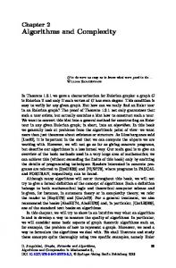
B. COMPARE Algorithm In this section, we propose and analyze a distributed algorithm that compares the total weight associated with two feasible schedules, π[t] and π ˜ [t], with local control signal transmissions, and choose the one with the larger weight as the schedule to be used during the next stage. In the following, we will omit the time index for ease of presentation. The algorithm relies on constructing the conflict graph associated with π and π ˜ which contains information about interfering links in the two schedules. The conflict graph, G 0 (π, π ˜ ) = (N 0 , L0 ), of π and π ˜ can be generated as follows10 : Each link l in π ∪ π ˜ corresponds to a node in the conflict graph, and if links l1 ∈ π and l2 ∈ π ˜ interfere with each other, an edge is drawn between the nodes corresponding to l1 and l2 in the conflict graph. Note that, since both π and π ˜ are feasible schedules, no two links in the same schedule (π or π ˜ ) can interfere with each other, i.e., there is no edge between two nodes of the same schedule in G 0 . Every node in G 0 can compute its own weight [as defined in (1)], and has a list of its neighbors in G 0 by part (iv) of Proposition 1. We will develop the algorithms using the conflict graph G 0 and show at the end of this section that the special structure enables us to map the operations to the graph G. Our C OMPARE Algorithm is composed of two procedures that are implemented consecutively: F IND S PANNING T REE and C OMMUNICATE & D ECIDE. The F IND S PANNING T REE procedure finds a spanning tree for each connected component of G 0 in a distributed fashion. Then, the C OMMUNICATE & D ECIDE procedure exploits the constructed tree structure to communicate and compare the weights of the two schedules in a distributed manner. To illustrate the definitions and operation of the algorithms we consider the grid network depicted in Figure 2. In this network, nodes are located on the corner points of a grid, and each interior node has four links incident to it. To demonstrate 10 We use N 0 , L0 to denote the cardinalities of N 0 , L0 . Also, we will refer to G 0 (π, π ˜ ) simply as G 0 for convenience.
the construction of the conflict graph, suppose we are given two feasible schedules, π and π ˜ . In the figure, solid bold links belong to schedule π, while dashed bold links are in π ˜ . We use dash-dotted thin lines to connect the links of the two schedules that interfere with each other. In general, it is not necessary that the conflict graph be connected. For example, in Figure 2, we observe six disconnected components. The conflict graph corresponding to the largest connected component is given in Figure 3, where links in π are drawn as circular dots, while links in π ˜ are drawn as square dots. Remark 1: Disconnected components of the conflict graph can decide on which schedule to use, independent of each other. This is possible because by construction of the conflict graph the resulting schedule is guaranteed to be feasible even if the choices of two disconnected components are different. This decomposition contributes to the distributed nature of the algorithm. Namely, the size of the graph within which the comparison is to be performed is likely to be reduced. Notice that with this approach, the chosen schedule may be a combination of the two candidate schedules, π and π ˜, because different connected components may prefer different schedules. This merging operation will result in a schedule that is better than both π and π ˜. Based on this remark, henceforth our algorithm will focus on the decision of a single connected component. 1) F IND S PANNING T REE Procedure: The object of the F IND S PANNING T REE procedure is to find, in a distributed fashion, a spanning tree for each of the connected components in the conflict graph. In our model, every node in the conflict graph G 0 corresponds to an undirected link in the original graph G, and has a unique ID11 . In order to compare two link IDs, we use lexicographical ordering12 . 11 In [11], it was shown that unique IDs are required to be able to find a spanning tree in a distributed fashion. 12 Without loss of generality, assume ID(n) < ID(m) and ID(i) < ID(j) : If ID(n) < ID(i), then ID(n, m) < ID(i, j) for all m, j; and if ID(n) = ID(i) and ID(m) < ID(j), then ID(n, m) < ID(i, j).
Our distributed F IND S PANNING T REE procedure is based on token generation and forwarding operations. For the construction of a spanning tree, at least one token needs to be generated within each connected component. This can be guaranteed by requiring every node in the conflict graph that has the lowest ID number among its neighbors to generate a token. Each token, carrying the ID of its generator, performs a depth-first traversal (cf. [6]) within the connected component to construct a spanning tree. This token progressively adds nodes into its spanning tree while avoiding the construction of cycles. An example is depicted in Figure 3 for the largest connected component of Figure 2. minimum token
1
3
2 � �
� �
� �
� �
� �
� �
4 �
�
�
�
�
�
5
X 6
7
� �
� �
� �
� �
� �
� �
9
8
�
�
�
�
�
�
The idea is to convey the necessary information from the leaves up to the root of the tree (i.e. C OMMUNICATE Procedure) so that the schedule with the higher weight is chosen (cf. (4)), and then send back the decision to the leaves (i.e. D ECIDE Procedure). The C OMMUNICATE & D ECIDE procedure can be explained in two parts as follows: C OMMUNICATE : The leaves communicate their weights to their parents. If the parent is in π it adds its weight to the sum of the weights announced by its children. If, on the other hand, it is in π ˜ it subtracts its weight from the sum of its children’s weights. The resulting value becomes the new weight of the parent. Then, the parent acts as a leaf with the updated weight in the next iteration. This recursive update is repeated until the root is reached. D ECIDE : At the end of C OMMUNICATE of P , the weight P the root of the spanning tree will be w − w l l∈π l∈˜ π l. Depending on whether the root’s weight is positive or negative, the root decides π or π ˜ , respectively, as the better schedule, and broadcasts its decision down the tree.
10 π
Σ wi i
� �
� �
� �
� �
� �
� �
∼
- Σ wπi i
11
12
... Fig. 3. A connected component of the conflict graph from which the link crossed is eliminated to obtain a spanning tree. The path of the minimum token is indicated with arrows. The nodes are labeled with numbers for future reference.
... ∼
13 f (n) = O(g(n)) means that there exists a constant c < ∞ such that f (n) ≤ cg(n) for n large enough.
∼
w2π- wπ 1 ∼
w1π
∼
w8π- wπ- wπ 6 7 ∼
w6π
∼
∼
∼
w8π+ w11π- wπ- wπ - wπ- wπ12 6 7 9
3
∼
The above procedure focuses on the operation of a single token generated at one of the nodes within the connected component. In general, there may be multiple tokens generated within the same connected component. Each token attempts to form its spanning tree labeled with its ID number (i.e. the ID number of the token’s generator). Since only one spanning tree is required at the end of the procedure, our algorithm is designed to keep the spanning tree with the smallest ID number, while eliminating the others. This elimination is performed when the token of a spanning tree enters a node that has been traversed by another token. If the incoming token has smaller ID, then the token ignores the previous token and continues the construction of its tree, and if its ID is larger, then it is immediately deleted. We have the following proposition for this algorithm (see [7] for the proof, which is omitted in the interest of space). Proposition 2: Consider the conflict graph G 0 = (N 0 , L0 ), and let D0 denote the maximum degree of G 0 . The F IND S PAN NING T REE Procedure finds a spanning tree of all components of the conflict graph in O(D0 L0 ) time13 , and with O(D0 N 0 ) message exchanges for each n0 ∈ N 0 . In particular, at the termination of the procedure, every node n0 ∈ N 0 has a list of its neighbors in the constructed spanning tree. 2) C OMMUNICATE & D ECIDE Procedure: We use the spanning tree formed on the conflict graph to compare weights.
∼
∼
w2π- wπ1 - wπ
∼
w7π
∼
w11π- wπ12 ∼
wπ12
Fig. 4. The iterative communication of the weights of the two schedules from the leaves to the root for the spanning tree of Figure 3.
An example of this procedure is provided in Figure 4 for the spanning tree given in Figure 3. We have the following complexity result for this procedure (see [7] for the proof). Proposition 3: Consider the conflict graph G 0 = (N 0 , L0 ), and let D0 denote the maximum degree of G 0 . The C OMMUNI CATE & D ECIDE procedure correctly finds the schedule with the larger weight in O(D0 L0 ) time. Notice that the complexity results in the propositions are given in terms of G 0 . We can translate them into bounds on G through the following inequalities: L0 < N 2 , D0 < N . Propositions 1, 2 and 3, together with Theorems 1 and 2 yields the following result. Theorem 3: The distributed implementations of P ICK and C OMPARE Algorithms designed for the two-hop interference model asymptotically achieve throughput-optimality and fairness with O(N 3 ) time and O(N 2 ) message exchanges per node, per stage. ¤
VI. S IMULATIONS In this section, we provide simulation results for the distributed algorithms developed in Section V for the grid topology (see Figure 2). We use the notation [i, j] to refer to the node at the ith row and j th column of the grid. Throughout, we simulate utility functions of the form Ui (x) = γi log(x), which corresponds to weighted proportionally fair allocation (see [13], [23]). Throughput evolution for 6x6 Network with 4 flows
Throughput achieved
0.25
0.2
0.15
0.1
Flow−1 Flow−2 Flow−3 Flow−4
0.05
0
0
1
2
3
4
5
6
Number of Stages
7
8
9
10 4
x 10
Fig. 5. The throughput evolution of the 6x6 network for K = 100, γi = 0.5.
We first consider a network of size 6x6, with four flows: Flow-1 from [1, 1] to [6, 6], Flow-2 from [5, 2] to [6, 3], Flow-
3 from [5, 5] to [5, 1], and Flow-4 from [4, 1] to [1, 4]. Here, we are interested in the evolution of the throughputs of each flow for K = 100 and γi = 0.5 for each i ∈ {1, 2, 3, 4}. The simulation results are depicted in Figure 5. We observe that the throughputs of the flows converge to different values depending on their source-destination separation. For example, Flow-2 achieves the highest throughput since its source is only two hops from its destination. The fluctuations in the evolutions are due to the random nature of the algorithm, which tracks the queue-length evolutions. 0.4
(0,1)
(.1,.9) (.2,.8)
(γ1,γ2)
(.3,.7)
0.35
(.4,.6) 0.3
Thoughput of Flow−2
Before we complete the section, we make a few important remarks on the operation and extension of the algorithms. Remark 2: The algorithms we develop in this section operate over the conflict graph G 0 . These operations can be transformed into operations in the actual graph G. Such a transformation would be difficult for a general conflict graph. However, in our scenario the graph has a special structure that enables the mapping. The critical observation is that transmissions within a feasible schedule has no interference. Thus, links that form π and π ˜ can perform operations in G 0 by partitioning CSI (cf. Figure 1) into two disjoint time intervals. During the first interval, only links that make up π communicate, while in the second interval only nodes that make up π ˜ communicate. The operation of each link can easily be mapped into operations at its two end nodes by assigning one node to each operation, who will then coordinate the operation. With such a separation of time, the operations described for the conflict graph can be translated into operations in the actual network. Remark 3: Recall from Remark 1 that the conflict graph is likely to be composed of multiple disconnected components, which increases the distributed nature of the algorithms. Even though we did not pursue this direction here, this likelihood can be increased by dynamically modifying the activation probabilities, {pn }n , in the P ICK Algorithm so that the picked schedule has more disconnected components. This way, the localized nature of the algorithm can be improved.
(.5,.5) (.6,.4)
0.25
(.7,.3) 0.2
(.8,.2) 0.15
(.9,.1) 0.1
K=100
0.05
K=10 0
0
0.05
0.1
0.15
0.2
K=20
K=40
0.25
0.3
K=60 0.35
K=80 0.4
0.45
Throughput of Flow−1
Fig. 6.
Throughputs of flows with varying K and (γ1 , γ2 ).
Next, we simulate a 10x10 network with two flows: Flow-1 from [1, 1] to [8, 9], and Flow-2 from [9, 2] to [2, 10]. Here, we focus on the throughputs achieved for the flows as a function of K with varying γi for each flow. We aim to observe the average flow rates as functions of K and (γ1 , γ2 ). Notice that each (γ1 , γ2 ) combination corresponds to a different weighting for the weighted-proportionally fair allocation. Thus, for a fixed K, the throughputs corresponding to different (γ1 , γ2 ) combinations actually outline the rate region that the algorithm achieves for that K. Then, as K grows Theorem 2 implies that this region grows at a decreasing rate, until it converges to the stability region Λ. We performed simulations for K varying from 10 to 100, and (γ1 , γ2 ) ranging from (0, 1) to (1, 0) with γ1 + γ2 = 1 at each intermediate point. The simulation results are provided in Figure 6. We observe that for a given K, the rate region is a convex region. Also, as K grows, the region expands at a decreasing rate agreeing with our expectations. We further note that with this algorithmic method, the stability region of a wireless network, that is otherwise difficult to find, can be determined with high accuracy. Finally, for the previous simulation setting, we fix K to 100 and vary (γ1 , γ2 ) as before, and compare the rate region achieved with our policy to the greedy distributed maximal scheduling policy proposed in earlier works [15], [4]. The greedy policy always picks a random maximal schedule, but does not perform any comparison with an earlier schedule. The two regions are plotted in Figure 7. We observe that there
Comparison of Stability regions for K=100 0.4
Our Policy Greedy Policy
0.35
Throughput of Flow−2
0.3
0.25
0.2
0.15
0.1
0.05
0
0
0.05
0.1
0.15
0.2
0.25
0.3
0.35
0.4
Throughput of Flow−1
Fig. 7.
Throughputs of flows with K = 100 and varying (γ1 , γ2 ).
is a considerable gain in throughput when our algorithm is implemented compared to the greedy algorithm. VII. C ONCLUSIONS In this work, we provided a framework for the design of cross-layer algorithms for full utilization of multi-hop wireless networks. We started with generalizing a practical randomized policy, first introduced in [25] for switches, to multi-hop networks. We proved that with a single comparison at each iteration, this policy achieves 100% of the available capacity of the network. Next, we considered the case of elastic flows and provided a decentralized congestion control algorithm that works in parallel with the randomized algorithm. We showed that the resulting cross-layer algorithm achieves fair allocation of the resources despite the imperfect nature of the schedulingrouting algorithm (i.e. the randomized algorithm does not always pick the maximum weighted schedule). Finally, we developed specific distributed algorithms for the two-hop interference model. For this model, existing throughput-optimal strategies require that an NP-hard problem be solved by a centralized controller at every time instant. In this work, we showed that this is not necessary, and full utilization of the network can be achieved with distributed algorithms having only polynomial communication and computational complexity. An important byproduct of our approach is the use of the developed cross-layer algorithms to find (with high accuracy) the stability region of ad-hoc wireless networks, that are otherwise difficult to characterize. R EFERENCES [1] M. Andrews, K. Kumaran, K. Ramanan, A. Stolyar, R. Vijayakumar, and P. Whiting. Scheduling in a queueing system with asynchronously varying service rates, 2000. Bell Laboratories Technical Report. [2] E. Arikan. Some complexity results about packet radio networks. IEEE Transactions on Information Theory, 30:681–685, 1984. [3] D. P. Bertsekas and J. N. Tsitsiklis. Parallel and Distributed Computation: Numerical Methods. Athena Scientific, Belmont, MA, 1997.
[4] L. Bui, A. Eryilmaz, R. Srikant, and X. Wu. Joint asynchronous congestion control and distributed scheduling for wireless networks. Proceedings of IEEE Infocom 2006. [5] P. Chaporkar, K. Kar, and S. Sarkar. Throughput guarantees through maximal scheduling in wireless networks. In Proceedings of the Allerton Conference on Control, Communications and Computing, 2005. [6] T. H. Cormen, C. E. Leiserson, R. L. Rivest, and C. Stein. Introduction to Algorithms. M.I.T. Press, McGraw-Hill, London, England, 2001. [7] A. Eryilmaz, A. Ozdaglar, and E. Modiano. Polynomial complexity algorithms for full utilization of multi-hop wireless networks, 2005. Technical Report, available at http://www.mit.edu/˜eryilmaz/research.html. [8] A. Eryilmaz and R. Srikant. Fair resource allocation in wireless networks using queue-length based scheduling and congestion control. In Proceedings of IEEE Infocom, vol. 3, pages 1794–1803, March 2005. [9] A. Eryilmaz and R. Srikant. Resource allocation of multi-hop wireless networks. In Proceedings of International Zurich Seminar on Communications, February 2006. [10] A. Eryilmaz, R. Srikant, and J. R. Perkins. Stable scheduling policies for fading wireless channels. IEEE/ACM Transactions on Networking, 13:411–425, April 2005. [11] R. G. Gallager, P. A. Humblet, and P. M. Spira. A distributed algorithm for minimum-weight spanning trees. ACM Transactions on Programming Languages and Systems, 5:66–77, 1983. [12] F. P. Kelly. Charging and rate control for elastic traffic. European Transactions on Telecommunications, 8:33–37, 1997. [13] F. P. Kelly, A. Maulloo, and D. Tan. Rate control in communication networks: Shadow prices, proportional fairness and stability. Journal of the Operational Research Society, 49:237–252, 1998. [14] X. Lin and N. Shroff. Joint rate control and scheduling in multihop wireless networks. In Proceedings of IEEE Conference on Decision and Control, Paradise Island, Bahamas, December 2004. [15] X. Lin and N. Shroff. The impact of imperfect scheduling on crosslayer rate control in multihop wireless networks. In Proceedings of IEEE Infocom, Miami, FL, March 2005. [16] S. H. Low and D. E. Lapsley. Optimization flow control, I: Basic algorithm and convergence. IEEE/ACM Transactions on Networking, 7:861–875, December 1999. [17] E. Modiano, D. Shah, and G. Zussman. Maximizing throughput in wireless networks via gossiping. In ACM SIGMETRICS/IFIP Performance, 2006. [18] M.J. Neely, E. Modiano, and C. Li. Fairness and optimal stochastic control for heterogeneous networks. In Proceedings of IEEE Infocom, pages 1723–1734, Miami, FL, March 2005. [19] M.J. Neely, E. Modiano, and C.E. Rohrs. Dynamic power allocation and routing for time varying wireless networks. In Proceedings of IEEE Infocom, pages 745–755, April 2003. [20] L. Peterson and B. Davie. Computer Networks: A Systems Approach. Morgan Kaufmann Publishers, Second edition, 2000. [21] G. Sasaki and B. Hajek. Link scheduling in polynomial time. IEEE Transactions on Information Theory, 32:910–917, 1988. [22] S. Shakkottai and A. Stolyar. Scheduling for multiple flows sharing a time-varying channel: The exponential rule. Translations of the AMS, Series 2, A volume in memory of F. Karpelevich, 207:185–202, 2002. [23] R. Srikant. The Mathematics of Internet Congestion Control. Birkh¨auser, Boston, MA, 2004. [24] A. Stolyar. Maximizing queueing network utility subject to stability: Greedy primal-dual algorithm. Queueing Systems, 50(4):401–457, 2005. [25] L. Tassiulas. Linear complexity algorithms for maximum throughput in radio networks and input queued switches. In Proceedings of IEEE Infocom, pages 533–539, 1998. [26] L. Tassiulas and A. Ephremides. Stability properties of constrained queueing systems and scheduling policies for maximum throughput in multihop radio networks. IEEE Transactions on Automatic Control, 36:1936–1948, December 1992. [27] X. Wu and R. Srikant. Regulated maximal matching: A distributed scheduling algorithm for multi-hop wireless networks with nodeexclusive spectrum sharing. In Proceedings of IEEE Conference on Decision and Control., 2005. [28] X. Wu and R. Srikant. Bounds on the capacity region of multi-hop wireless networks under distributedgreedy scheduling. In Proceedings of IEEE Infocom, 2006. [29] H. Yaiche, R. R. Mazumdar, and C. Rosenberg. A game-theoretic framework for bandwidth allocation and pricing in broadband networks. IEEE/ACM Transactions on Networking, 8(5):667–678, October 2000.