Polynomial Dynamic Time Warping Kernel Support Vector Machines ...

INTERSPEECH 2005

Polynomial Dynamic Time Warping Kernel Support Vector Machines for Dysarthric Speech Recognition with Sparse Training Data Vincent Wan, James Carmichael Department of Computer Science University of Sheffield, Sheffield, UK {v.wan,j.carmichael}@dcs.shef.ac.uk

Abstract

chine learning algorithms, including Gaussian mixture models, they can be made to classify variable length sequences directly and without the aid of a finite state machine (such as HMMs) to capture the temporal information. In this paper, sequence classification is achieved via the well known DTW algorithm, described in section 2. That section also discusses the concept of sequence kernels and introduces the notation used. The formulation of the novel polynomial DTW kernel is outlined in section 3. Experiments comparing the DTW-SVM to a standard DTW system and to a statistical HMM system are described in section 4 and the results presented in 5. Section 6 concludes the paper.

This paper describes a new formulation of a polynomial sequence kernel based on dynamic time warping (DTW) for support vector machine (SVM) classification of isolated words given very sparse training data. The words are uttered by dysarthric speakers who suffer from debilitating neurological conditions that make the collection of speech samples a timeconsuming and low-yield process. Data for building dysarthric speech recognition engines are therefore limited. Simulations show that the SVM based approach is significantly better than standard DTW and hidden Markov model (HMM) approaches when given sparse training data. In conditions where the models were constructed from three examples of each word, the SVM approach recorded a 45% lower error rate (relative) than the DTW approach and a 35% lower error rate than the HMM approach.

2. Background 2.1. Dynamic Time Warping In symmetric DTW [4] a global distance D(X, Y ) between two sequences of vectors X = {x1 , . . . , xNX } and Y = {y1 , . . . , yNY } is determined. In speech recognition tasks, x and y are vectors of cepstral coefficients and N is the the number of vectors in each sequence. Let the local distance be the Euclidean distance between two cepstral vectors, d(xi , yj ) = ||xi − yj ||. Since the two sequences may not be of equal length, an alignment must be defined so that each vector in X is matched with a corresponding vector in Y . This alignment is denoted by φx (k) and φy (k) for k = {1, · · · , K}, where K is the length of the alignment. Using this notation, xφx (k) is matched with yφy (k) . For the purpose of this work, the alignment maintains the temporal sequence within X and Y and no vectors may be omitted. The DTW alignment distance is determined for a given alignment by summing the local distances between matched vectors,

1. Introduction Hidden Markov model (HMM)-based speech recognition systems require a reasonable quantity of training data in order to perform well in real conditions. It is not always possible, however, to collect sufficient data to achieve the desired accuracy. Classification of dysarthric speech is an example of such a task where training corpora are usually severely limited. Debilitating neurological conditions which often accompany dysarthria can make the collection of speech samples from patients a time-consuming and low-yield process [1]. It is often not feasible, therefore, to provide ample corpora for training statistical speech recognition engines. Off-the-shelf HMM speech recognition systems typically employ pretrained models that are, to some extent, speaker-adaptable. Such systems, however, usually record unacceptably high error rates [2] when decoding speech resulting from certain types of dysarthria, particularly the progressive varieties where the patient’s pronunciation becomes increasingly dissimilar from the population norm as articulator control worsens. The usual solution to accommodate variability – training on larger corpora – is not applicable in this instance. This paper presents an isolated word recognition system based on the support vector machine (SVM) with a polynomial dynamic time warping (DTW) kernel (DTW-SVM) for the classification of dysarthric speech. This work is an advancement on the efforts of Green et al. [1]. It has been shown that support vector machines (SVMs) [3] generalise well on sparse training data. Unlike some other ma-

Dalign (X, Y ) =

K 1 X d(xφx (k) , yφy (k) ) K k=1

(1)

The global distance is the alignment distance along the Viterbi path, which is defined by D(X, Y ) = min Dalign (X, Y ).

(2)

A dynamic programming beam search is used to compute the global distance efficiently. 2.2. Support Vector Machines A support vector machine, as described in [5], is a general data classification technique for binary decision problems. The objective is to define a linear boundary that is “midway” between

This work was partly supported by the European Union 6th FWP IST Integrated Project AMI (Augmented Multi-party Interaction), FP6506811, publication AMI-67.

3321

September, 4-8, Lisbon, Portugal

INTERSPEECH 2005

x

two given data groups: the concept is known as margin maximisation. The data points closest to the decision boundary are known as the support vectors since they alone among all the data points define the hyperplane’s exact position. The maximum margin criterion makes the SVM particularly suitable for recognition tasks with limited training data. Although the SVM is based upon a linear discriminator, it is not restricted to making linear hypotheses. Non-linear decisions are made possible by a non-linear mapping of the data to a higher dimensional space. The phenomenon is analogous to folding a flat sheet of paper into any three-dimensional shape and then cutting it into two halves, the resultant non-linear boundary in the two-dimensional space is revealed by unfolding the pieces. The SVM’s non-parametric mathematical formulation allows these transformations to be applied efficiently and implicitly: the SVM’s objective is a function of the dot product between pairs of vectors; the substitution of the original dot products with those computed in another space eliminates the need to transform the original data points explicitly to the higher space. The computation of dot products between vectors without explicitly mapping to another space is performed by a kernel function, examples of such include the radial basis function kernel, « „ 1 2 (3) KRBF (x, y) = exp − 2 (x − y) 2σ

H

dS(^x,^y) a ^x

^y q^x,^y centre of S

S

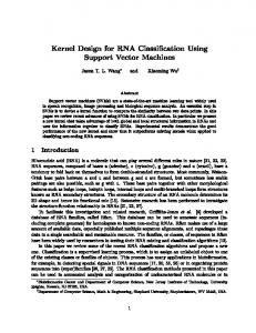
Figure 1: Converting a measure of distance to a dot product.

the sampled vectors x and y normally exist, represented in the figure as a straight line. Let S be a unit hypersphere embedded in a space that has one dimension more than H. Consider two points in H represented by vectors x and y. The spherical normalisation procedure projects each point along the dotted lines onto the surface of S. Each projected point ˆ and y ˆ that originate from the is represented by unit vectors x ˆ is centre of S. The formula for the transformation from x to x » – 1 x ˆ= √ (5) x x2 + α2 α

and the polynomial kernel, Kpoly (x, y) = (x · y)n

y

where α is the perpendicular distance from the centre of S to H. Since the transformation is reversible, there is no loss of information. A detailed description of the properties of spherical normalisation can be found in [11]. ˆ = {ˆ ˆ NX } denote the sequence X after it is Let X x1 , . . . , x mapped onto S and let Yˆ be similarly defined. It is in this new space that distances can be converted readily to dot products. ˆ ), of the geodesic on a unit x, y By definition, the length, dS (ˆ ˆ and hypersphere between two points represented by vectors x ˆ , equals the angle between the two vectors, θxˆ ,ˆy . Instead of y a Euclidean distance, therefore, let the local DTW distance be the shortest distance between two points on the surface of the hypersphere, ˆ ) = θxˆ ,ˆy dS (ˆ x, y (6)

(4)

where σ is the width of the radial basis functions and n is the order of the polynomial. 2.3. Sequence kernels A sequence kernel is a function that operates on two complete sequences. They enable SVMs to perform discriminative classification of sequences of unequal length directly at the sequencelevel. This contrasts with HMM-based techniques where sequences are divided into frames and discrimination is then applied at the frame-level, potentially resulting in the loss of information useful for sequence-level classification. Examples of sequence kernels include the Fisher kernel [6], the pair HMM kernel [7] and the generalised linear discriminant kernel [8]. The well known DTW approach provides a way of computing a ‘distance’ between two sequences that can be exploited to derive sequence kernels. In the approach by Shimodaira et al. [9], the local distance in the DTW algorithm was substituted with a similarity measure defined by the right-hand side of (3) and the global distance redefined to maximise the similarity. However, the resulting alignment path found by this method differs significantly from that obtained when using the Euclidean local distance metric, a factor which can negatively influence recognition accuracy. An alternative approach by Bahlmann et al. [10] kept the Euclidean local distance and replaced the (x − y) term in (3) with the DTW global distance thereby creating a ‘radial basis function DTW kernel’.

ˆ ·y ˆ = cos θxˆ ,ˆy , the new local DTW distance Using the relation x may be expressed in terms of a dot product, ˆ ) = arccos(ˆ ˆ) dS (ˆ x, y x·y

(7)

The same principle can be used to reconvert the DTW global distance measured in S to a dot product, ˆ Yˆ ) = cos DS (X, ˆ Yˆ ) Klinear DTW (X,

(8)

where DS is the global distance computed using the local distance defined by (7). It is important to note that (8) can only be a valid kernel ˆ Yˆ ) = if the symmetric form of DTW is used, i.e. DS (X, ˆ In addition to symmetry, the kernel function must DS (Yˆ , X). satisfy Mercer’s condition [13] or be proven by alternative means to be a valid dot product. By definition, the cosine of the angle between two unit vectors is guaranteed to yield a dot product. From equations (1) and (6), the global distance is the mean of the angles between the pairs of vectors from the two sequences. However, it may be disputed whether the cosine of such a mean is still a dot product. Our simulations have not

3. Polynomial DTW kernel The method employed herein for converting the DTW global distance to a dot product uses a technique called spherical normalisation [11, 12] and the polynomial kernel (4). Figure 1 illustrates the process of derivation. Let H be the space in which

3322

INTERSPEECH 2005

40

encountered any of the expected convergence anomalies if the kernel were invalid. Assuming that equation (8) is a valid dot product, it can be substituted into equation (4), replacing the term (x · y) to obtain higher order non-linear solutions. Thus the polynomial DTW kernel takes the form,

Recognition error rate (%)

ˆ Yˆ ) = cosn DS (X, ˆ Yˆ ) Kpoly DTW (X,

35

(9)

The procedure for computing the polynomial DTW kernel is summarised as follows: 1. Map the vectors of each sequence to a hypersphere using equation (5).

DT

W, dy

sar t

hri c

30 HM

25

M

,d

ys

20 SVM

art

hr

ic

, dy

15

sart hric

10

2. Perform DTW to get the global distance as defined by equation (2) using the local distance defined by equation (7).

DTW, normal HMM, normal

5

SVM, normal

3. Take the cosine of the global distance and raise to the nth power according to equation (9).

0 3

4. Experiments

4

5 6 7 8 9 10 11 12 13 14 Number of training examples per word

15

Figure 2: The error rates of DTW-SVMs, HMMs and standard DTW systems on normal and dysarthric speakers as a function the size of the training set.

Isolated word speech recognition simulations were performed using speech collected from both normal and dysarthric speakers [1]. This is necessarily a speaker dependent task because dysarthric speech can differ enormously between speakers depending upon the severity of their disability. There were 7 dysarthrics and 7 non-dysarthrics, each uttering between 30 and 40 examples of each of the words: alarm, lamp, radio, TV, channel, volume, up, down, on and off. Given the limited quantity of data, N -fold cross-validation was used to increase the number of tests performed so that statistically significant results could be obtained. Cross-validation was performed using training set sizes ranging from 3 to 15 examples per word as follows: for each specified training set size, that number of utterances were randomly selected for model building and the remaining utterances were used for testing; this process was repeated until all of the utterances were selected once for training. This yielded over 17000 individual tests on dysarthric speech when training sets were at the 3-sample minimum and approximately 1700 when training corpus size was maximised to 15 utterances per words. The speech was parameterised using 13 Mel-frequency cepstral coefficients (MFCCs) computed using a 32 millisecond window with a 10 millisecond frame shift, augmented with their first order derivatives and normalised to zero mean and unit diagonal covariance resulting in vectors of 26 dimensions. A Gaussian mixture silence detector, employing smoothing techniques, was used to remove all frames representing silence or containing short bursts of non-speech noise. Three word modelling techniques were compared. The first was a standard DTW system. It used all the utterances in the training selection as its templates and classified a test utterance according to the single closest matching template. The training utterances were manually end-pointed to contain only the relevant speech. During testing, this system required the use of a detector to remove frames of silence. The second technique was the HMM system, Stardust1 , implemented in [15], employing a silence-word-slience grammar, using a continuous density ‘straight-through’ model topology

11-state HMM with 3 Gaussians per state. The silence models also captured any other non-speech noises in the audio. The third was the polynomial DTW-SVM described in section 3. SVMs are binary classifiers so the directed acyclic graphs approach [16] was used to achieve multi-class classification. That approach considers the classes in pairs: an SVM trained to discriminate between those two classes is used to eliminate one of them. The process is repeated until one class remains. Like the standard DTW system, the training utterances were manually end-pointed and the test utterances were stripped of silence frames using an automatic detector.

5. Results Trials on the DTW-SVM system showed that good accuracy could be achieved using a third order polynomial, where n = 3 in (9) and α = 1 in (5). In these simulations, the SVMs were set up to classify separable data (i.e. the regularisation parameter, or upperbound on the Lagrange multipliers, was set to infinity). The average Lagrange multiplier value was of the order 0.1 with maximum values in the range 1 to 5. Due to the paucity of training data, the SVM solutions – save a few exceptions – used all of the training data for support vectors. A summary of the results is shown in figure 2. The standard DTW system returned the highest error rate across all conditions. Results on normal speech showed no significant difference between the DTW-SVM and HMM techniques except when training sets were reduced to 3 examples per word; when so constrained, the SVMs reduced the error rate to 4.0% compared to the HMM’s 7.4%, a 46% relative reduction. On dysarthric speech, when trained on 3 examples per word, the DTW-SVM system had a 19.7% error rate and the HMM 30.1%, a relative reduction of 35%. When training corpus size ranged from 6 to 15 samples per model, the SVM continued to outperform the HMM, with the difference in respective

1 This system was built around the HTK toolkit [14] using a multipass re-estimation strategy that was bootstrapped from manually endpointed speech.

3323

INTERSPEECH 2005

error rates remaining roughly constant at about 2% absolute.

[9] H. Shimodaira, K. Noma, M. Nakai, and S. Sagayama, “Support vector machine with dynamic time-alignment kernel for speech recognition,” in Proc. Eurospeech, 2001.

6. Conclusion

[10] C. Bahlmann, B. Haasdonk, and H. Burkhardt, “On-line handwriting recognition with support vector machines – a kernel approach,” in Proc. 8th International Workshop on Frontiers in Handwriting Recognition, 2002, pp. 49–54.

A novel polynomial DTW kernel SVM was presented in this paper. The new kernel was obtained by converting the DTW distance measure between two sequences into a kernel function appropriate for an SVM. Simulations compared the DTW-SVM with standard DTW and HMM techniques. The new approach was consistently more accurate than both standard DTW and HMM systems when presented with the sparse training data from dysarthric speakers. In tests on normal speech, there was no observable difference in accuracy between the HMM and DTW-SVM techniques except in one condition when the training data was most sparse. In that single condition, the DTW-SVM yielded its greatest relative (46%) reduction in the error rate compared to the HMM. This improvement is of more than just academic interest for this research team: the next phase of investigation will involve the production of a speech-activated environmental control system (SPECS) which, unlike its predecessor, will progress beyond proof-of-concept stage and become a commercially available product. The DTW-SVM’s performance qualifies this technology as a candidate for the SPECS speech recognition engine, a possibility which would represent a refreshing alternative to HMM statistical modelling which seems to predominate the research effort in this domain.

[11] V. Wan, Speaker Verification using Support Vector Machines, Ph.D. thesis, University of Sheffield, June 2003. [12] V. Wan and S. Renals, “Speaker verification using sequence discriminant support vector machines,” IEEE Transactions on Speech and Audio Processing, vol. 13, no. 2, pp. 203–210, March 2005. [13] R. Courant and D. Hilbert, Physics, Interscience, 1953.

Methods of Mathematical

[14] S. J. Young, “The HTK HMM toolkit: Design and philosopy.,” Tech. Rep., Univ. Cambridge, Dept. Eng., 1993. [15] A. Hatzis, P. Green, J. Carmichael, S. Cunningham, R. Palmer, M. Parker, and P. O’Neil, “An integrated toolkit deploying speech technology for computer based speech training to dysarthric speakers,” in Proc. Eurospeech, 2003, pp. 2213–2216. [16] J. Platt, N. Cristianini, and J. Shawe-Taylor, “Large margin DAGs for multiclass classification,” in Advances in Neural Information Processing Systems 12, 2000.

7. Acknowledgements The authours would like to thank Roger Moore for his guidance and contributions.

8. References [1] P. Green, J. Carmichael, A. Hatzis, P. Enderby, M. Hawley, and M. Parker, “Automatic speech recognition with sparse training data for dysarthric speakers,” in Proc. Eurospeech, 2003. [2] J. Deller, D. Hsu, and L. Ferrier, “On the use of hidden Markov modelling for recognition of dysarthric speech,” in Computer Methods and Programmes in Biomedicine, 1991, vol. 35, pp. 125–139. [3] B. Sch¨olkopf, C. Burges, and A. Smola, Eds., Advances in Kernel Methods — Support Vector Learning, MIT Press, 1999. [4] L. Rabiner and B. H. Juang, Fundamentals of Speech Recognition, Prentice Hall, 1993. [5] C. J. C. Burges, “A tutorial on support vector machines for pattern recognition,” Data Mining and Knowledge Discovery, vol. 2, no. 2, pp. 1–47, 1998. [6] T. S. Jaakkola and D. Haussler, “Exploiting generative models in discriminative classifiers,” in Advances in Neural Information Processing Systems 11, M. S. Kearns, S. A. Solla, and D. A. Cohn, Eds. MIT Press, 1998. [7] C. Watkins, “Dynamic alignment kernels,” Tech. Rep., Royal Holloway College, University of London, 1999. [8] W. M. Campbell, “Generalised linear disciminant sequence kernels for speaker recognition,” in Proc. ICASSP, 2002.

3324