Jul 29, 2016 - performance and it is necessary to consider additional form .... js. = ât =tãut s , xiãxji efficiently. If for all i â [n] and for t and s fixed, we ..... ANOVA kernel vs. polynomial kernel. .... Scikit-learn: Machine learning in Python.
arXiv:1607.08810v1 [stat.ML] 29 Jul 2016
Polynomial Networks and Factorization Machines: New Insights and Efficient Training Algorithms
Mathieu Blondel MATHIEU . BLONDEL @ LAB . NTT. CO . JP Masakazu Ishihata ISHIHATA . MASAKAZU @ LAB . NTT. CO . JP Akinori Fujino FUJINO . AKINORI @ LAB . NTT. CO . JP Naonori Ueda UEDA . NAONORI @ LAB . NTT. CO . JP NTT Communication Science Laboratories, 2-4 Hikaridai Seika-cho Soraku-gun, Kyoto 619-0237, Japan
Abstract Polynomial networks and factorization machines are two recently-proposed models that can efficiently use feature interactions in classification and regression tasks. In this paper, we revisit both models from a unified perspective. Based on this new view, we study the properties of both models and propose new efficient training algorithms. Key to our approach is to cast parameter learning as a low-rank symmetric tensor estimation problem, which we solve by multi-convex optimization. We demonstrate our approach on regression and recommender system tasks.
1. Introduction Interactions between features play an important role in many classification and regression tasks. One of the simplest approach to leverage such interactions consists in explicitly augmenting feature vectors with products of features (monomials), as in polynomial regression. Although fast linear model solvers can be used (Chang et al., 2010; Sonnenburg & Franc, 2010), an obvious drawback of this kind of approach is that the number of parameters to estimate scales as O(dm ), where d is the number of features and m is the order of interactions considered. As a result, it is usually limited to second or third-order interactions. Another popular approach consists in using a polynomial kernel so as to implicitly map the data via the kernel trick. The main advantage of this approach is that the number of parameters to estimate in the model is actually independent of d and m. However, the cost of storing and evaluating the model is now proportional to the number of training instances. This is sometimes called the curse of kernelization (Wang et al., 2010). Common ways to address the issue inProceedings of the 33 rd International Conference on Machine Learning, New York, NY, USA, 2016. JMLR: W&CP volume 48. Copyright 2016 by the author(s).
clude the Nystr¨om method (Williams & Seeger, 2001), random features (Kar & Karnick, 2012) and sketching (Pham & Pagh, 2013; Avron et al., 2014). In this paper, in order to leverage feature interactions in possibly very high-dimensional data, we consider models which predict the output y ∈ R associated with an input vector x ∈ Rd by yˆK (x; λ, P ) :=
k X s=1
λs K(ps , x),
(1)
where λ = [λ1 , . . . , λk ]T ∈ Rk , P = [p1 , . . . , pk ] ∈ Rd×k , K is a kernel and k is a hyper-parameter. More specifically, we focus on two specific choices of K which allow us to use feature interactions: the homogeneous polynomial and the ANOVA kernels. Our contributions are as follows. We show (Section 3) that choosing one kernel or the other allows us to recover polynomial networks (PNs) (Livni et al., 2014) and, surprisingly, factorization machines (FMs) (Rendle, 2010; 2012). Based on this new view, we show important properties of PNs and FMs. Notably, we show for the first time that the objective function of arbitrary-order FMs is multi-convex (Section 4). Unfortunately, the objective function of PNs is not multiconvex. To remedy this problem, we propose a lifted approach, based on casting parameter estimation as a lowrank tensor estimation problem (Section 5.1). Combined with a symmetrization trick, this approach leads to a multiconvex problem, for both PNs and FMs (Section 5.2). We demonstrate our approach on regression and recommender system tasks. Notation. We denote vectors, matrices and tensors using lower-case, upper-case and calligraphic bold, e.g., w, W m times z }| { and W. We denote the set of d × · · · × d real tensors by m m Rd and the set of symmetric real tensors by Sd . We use h·, ·i to denote vector, matrix and tensor inner product. Given x, we define a symmetric rank-one tensor by
Polynomial Networks and Factorization Machines: New Insights and Efficient Training Algorithms m
x⊗m := x ⊗ · · · ⊗ x ∈ Sd , where (x⊗m )j1 ,j2 ,...,jm = xj1 xj2 . . . xjm . We use [d] to denote the set {1, . . . , d}.
2. Related work
Hm (p, x) := P0m (p, x) = hp, xim . Let p = [p1 , . . . , pd ]T and x = [x1 , . . . , xd ]T . Then,
2.1. Polynomial networks Polynomial networks (PNs) (Livni et al., 2014) of degree m = 2 predict the output y ∈ R associated with x ∈ Rd by yˆPN (x; w, λ, P ) := hw, xi + hσ(P T x), λi,
(2)
where w ∈ R , P ∈ R , λ ∈ R and σ(u) := u is evaluated element-wise. Intuitively, the right-hand term can be interpreted as a feedforward neural network with one hidden layer of k units and with activation function σ(u). Livni et al. (2014) also extend (2) to the case m = 3 and show theoretically that PNs can approximate feedforward networks with sigmoidal activation. A similar model was independently shown to perform well on dependency parsing (Chen & Manning, 2014). Unfortunately, the objective function of PNs is non-convex. In Section 5, we derive a multi-convex objective based on low-rank symmetric tensor estimation, suitable for training arbitrary-order PNs. d
where m ∈ N is the degree and γ > 0 is a hyper-parameter. We define the homogeneous polynomial kernel by
d×k
k
2
2.2. Factorization machines One of the simplest way to leverage feature interactions is polynomial regression (PR). For example, for second-order interactions, in this approach, we compute predictions by X yˆPR (x; w, W ) := hw, xi + W j,j 0 xj xj 0 , j 0 >j
2
where w ∈ Rd and W ∈ Rd . Obviously, model size in PR does not scale well w.r.t. d. The main idea of (secondorder) factorization machines (FMs) (Rendle, 2010; 2012) is to replace W with a factorized matrix P P T : X yˆFM (x; w, P ) := hw, xi + (P P T )jj 0 xj xj 0 , j 0 >j
where P ∈ R . FMs have been increasingly popular for efficiently modeling feature interactions in highdimensional data, see (Rendle, 2012) and references therein. In Section 4, we show for the first time that the objective function of arbitrary-order FMs is multi-convex. d×k
3. Polynomial and ANOVA kernels
Hm (p, x) =
d X j1 =1
...
d X
pj1 xj1 . . . pjm xjm .
jm =1
We thus see that Hm uses all monomials of degree m (i.e., all combinations of features with replacement). A much lesser known kernel is the ANOVA kernel (Stitson et al., 1997; Vapnik, 1998). Following (Shawe-Taylor & Cristianini, 2004, Section 9.2), the ANOVA kernel of degree m, where 2 ≤ m ≤ d, can be defined as X Am (p, x) := pj1 xj1 . . . pjm xjm . (3) jm >···>j1
As a result, Am uses only monomials composed of distinct features (i.e., feature combinations without replacement). For later convenience, we also define A0 (p, x) := 1 and A1 (p, x) := hp, xi.
With Hm and Am defined, we are now in position to state the following lemma. Lemma 1 Expressing PNs and FMs using kernels Let yˆK (x; λ, P ) be defined as in (1). Then, yˆPN (x; w, λ, P ) = hw, xi + yˆH2 (x; λ, P )
yˆFM (x; w, P ) = hw, xi + yˆA2 (x; 1, P ).
The relation easily extends to higher orders. This new view allows us to state results that will be very useful in the next sections. The first one is that Hm and Am are homogeneous functions, i.e., they satisfy λm K(p, x) = K(λp, x) ∀λ ∈ R, ∀m ∈ N+ . Another key property of Am (p, x) is multi-linearity.1 Lemma 2 Multi-linearity of Am (p, x) w.r.t. p1 , . . . , pd Let p, x ∈ Rd , j ∈ [d] and 1 ≤ m ≤ d. Then,
Am (p, x) = Am (p¬j , x¬j ) + pj xj Am−1 (p¬j , x¬j )
In this section, we show that the prediction functions used by polynomial networks and factorization machines can be written using (1) for a specific choice of kernel.
where p¬j denotes the (d − 1)-dimensional vector with pj removed and similarly for x¬j .
The polynomial kernel is a popular kernel for using combinations of features. The kernel is defined as
That is, everything else kept fixed, Am (p, x) is an affine function of pj , ∀j ∈ [d]. Proof is given in Appendix B.1.
Pγm (p, x) := (γ + hp, xi)m ,
1 A function f (θ1 , . . . , θk ) is called multi-linear (resp. multiconvex) if it is linear (resp. convex) w.r.t. θ1 , . . . , θk separately.
Polynomial Networks and Factorization Machines: New Insights and Efficient Training Algorithms
Assuming p is dense and x sparse, the cost of naively computing Am (p, x) by (3) is O(nz (x)m ), where nz (x) is the number of non-zero features in x. To address this issue, we will make use of the following lemma for computing Am in nearly O(mnz (x)) time when m ∈ {2, 3}. Lemma 3 Efficient computation of ANOVA kernel � 1 � 2 A2 (p, x) = H (p, x) − D2 (p, x) 2 � 1 � 3 A3 (p, x) = H (p, x) − 3D2,1 (p, x) + 2D3 (p, x) 6 Pd m where we defined Dm (p, x) := and j=1 (pj xj ) Dm,n (p, x) := Dm (p, x)Dn (p, x). See Appendix B.2 for a derivation.
4. Direct approach Let us denote the training set by X = [x1 , . . . , xn ] ∈ Rd×n and y = [y1 , . . . , yn ]T ∈ Rn . The most natural approach to learn models of the form (1) is to directly choose λ and P so as to minimize some error function n X DK (λ, P ) := ` (yi , yˆK (xi ; λ, P )) , (4)
5. Lifted approach 5.1. Conversion to low-rank tensor estimation problem If we set K = Hm in (4), the resulting optimization problem is neither convex nor multi-convex w.r.t. P . In (Blondel et al., 2015), for m = 2, it was proposed to cast parameter estimation as a low-rank symmetric matrix estimation problem. A similar idea was used in the context of phase retrieval in (Cand`es et al., 2013). Inspired by these works, we propose to convert the problem of estimating λ and P to m that of estimating a low-rank symmetric tensor W ∈ Sd . Combined with a symmetrization trick, this approach leads to an objective that is multi-convex, for both K = Am and K = Hm (Section 5.2). We begin by rewriting the kernel definitions using rank-one tensors. For Hm (p, x), it is easy to see that Hm (p, x) = hp⊗m , x⊗m i.
(5)
For Am (p, x), we need to ignore irrelevant monomials. For convenience, we introduce the following notation: X m hW, X i> := W j1 ,...,jm X j1 ,...,jm ∀ W, X ∈ Sd . jm >···>j1
i=1
where `(yi , yˆi ) is a convex loss function. Note that (4) is a convex objective w.r.t. λ regardless of K. However, it is in general non-convex w.r.t. P . Fortunately, when K = Am , we can show that (4) is multi-convex. Theorem 1 Multi-convexity of (4) when K = Am DAm is convex in λ and in each row of P separately.
We can now concisely rewrite the ANOVA kernel as Am (p, x) = hp⊗m , x⊗m i> .
(6)
Our key insight is described in the following lemma. Lemma 5 Link between tensors and kernel expansions m
Proof is given in Appendix B.3. As a corollary, the objective function of FMs of arbitrary order is thus multi-convex. Theorem 1 suggests that we can minimize (4) efficiently when K = Am by solving a succession of convex problems w.r.t. λ and the rows of P . We next show that when m is odd, we can just fix λ = 1 without loss of generality. Lemma 4 When is it useful to fit λ? Let K = Hm or Am . Then λ∈Rk ,P ∈Rd×k
min
DK (λ, P ) = min DK (1, P ) if m is odd.
λ∈Rk ,P ∈Rd×k
W=
P ∈Rd×k
P ∈Rd×k
The result stems from the fact that Hm and Am pare homogeneous functions. If we define v := sign(λ) m |λ|p, then we obtain λHm (p, x) = Hm (v, x) ∀λ if m is odd, and similarly for Am . That is, λ can be absorbed into v without loss of generality. When m is even, λ < 0 cannot be absorbed unless we allow complex numbers. Because FMs fix λ = 1, Lemma 4 shows that the class of functions that FMs can represent is possibly smaller than our framework.
k X
λs p⊗m s .
(7)
s=1
Let λ = [λ1 , . . . , λk ]T and P = [p1 , . . . , pk ]. Then, hW, x⊗m i = yˆHm (x; λ, P ) ⊗m
DK (λ, P ) ≤ min DK (1, P ) if m is even
min
Let W ∈ Sd have a symmetric outer product decomposition (Comon et al., 2008)
hW, x
i> = yˆ
Am
(8)
(x; λ, P ).
(9)
The result follows immediately from (5) and (6), and from m the linearity of h·, ·i and h·, ·i> . Given W ∈ Sd , let us define the following objective functions LHm (W) :=
n X i=1
LAm (W) :=
n X i=1
` yi , hW, x⊗m i i
�
� ` yi , hW, x⊗m i> . i
If W is decomposed as in (7), then from Lemma 5, we obtain LK (W) = DK (λ, P ) for K = Hm or Am . This
Polynomial Networks and Factorization Machines: New Insights and Efficient Training Algorithms
suggests that we can convert the problem of learning λ and P to that of learning a symmetric tensor W of (symmetric) rank k. Thus, the problem of finding a small number of bases p1 , . . . , pk and their associated weights λ1 , . . . , λk is converted to that of learning a low-rank symmetric tensor. Following (Cand`es et al., 2013), we call this approach lifted. Intuitively, we can think of W as a tensor that contains the weights for predicting y of monomials of degree m. For instance, when m = 3, W i,j,k is the weight corresponding to the monomial xi xj xk . 5.2. Multi-convex formulation m
Estimating a low-rank symmetric tensor W ∈ Sd for arbitrary integer m ≥ 2 is in itself a difficult non-convex problem. Nevertheless, based on a symmetrization trick, we can convert the problem to a multi-convex one, which we can easily minimize by alternating minimization. We first present our approach for the case m = 2 to give intuitions then explain how to extend it to m ≥ 3. Intuition with the second-order case. For the case m = 2, we need to estimate a low-rank symmetric matrix W ∈ 2 Sd . Naively parameterizing W = P diag(λ)P T and solving for λ and P does not lead to a multi-convex formulation for the case K = H2 . This is due to the fact that hP diag(λ)P T , x⊗2 i is quadratic in P . Our key idea is to parametrize W = S(U V T ) where U , V ∈ Rd×r and 2 S(M ) := 12 (M + M T ) ∈ Sd is the symmetrization of 2 M ∈ Rd . We then minimize LK (S(U V T )) w.r.t. U , V .
The main advantage is that both hS(U V T ), ·i and hS(U V T ), ·i> are bi-linear in U and V . This implies that LK (S(U V T )) is bi-convex in U and V and can therefore be efficiently minimized by alternating minimization. Once we obtained W = S(U V T ), we can optionally compute its eigendecomposition W = P diag(λ)P T , with k = rank(W ) and r ≤ k ≤ 2r, then apply (8) or (9) to obtain the model in kernel expansion form. Extension to higher-order case. For m ≥ 3, we now esm timate a low-rank symmetric tensor W = S(M) ∈ Sd , m where M ∈ Rd and S(M) is the symmetrization of M (cf. Appendix A.2). We decompose M using m matrices of size d × r. Let us call these matrices {U t }m t=1 and their columns uts = [ut1s , . . . , utds ]T . Then the decomposition of M can be expressed as a sum of rank-one tensors r X M= u1s ⊗ · · · ⊗ um (10) s . s=1
Due to multi-linearity of (10) w.r.t. U 1 , . . . , U m , the objective function LK is multi-convex in U 1 , . . . , U m . Computing predictions efficiently. When K = Hm , predictions are computed by hW, x⊗m i. To compute them efficiently, we use the following lemma.
Lemma 6 Symmetrization does not affect inner product hS(M), X i = hM, X i
m
m
∀ M ∈ Rd , X ∈ Sd , m ≥ 2. (11) m
Proof is given in Appendix A.2. Using x⊗m ∈ Sd , W = S(M) and (10), we then obtain hW, x⊗m i = hM, x⊗m i =
r Y m X
huts , xi.
s=1 t=1
As a result, we never need to explicitly compute the symmetrized tensor. For the case K = A2 , cf. Appendix D.3.
6. Regularization In some applications, the number of bases or the rank constraint are not enough for obtaining good generalization performance and it is necessary to consider additional form of regularization. For the lifted objective with K = H2 or A2 , we use the typical Frobenius-norm regularization ˜ K (U , V ) := LK (S(U V T ))+ β (kU k2F +kV k2F ), (12) L 2 where β > 0 is a regularization hyper-parameter. For the direct objective, we introduce the new regularization k X ˜ K (λ, P ) := DK (λ, P ) + β D |λs | kps k2 . (13) s=1
This allows us to regularize λ and P with a single hyperparameter. Let us define the following nuclear norm penalized objective: ¯ K (M ) := LK (S(M )) + βkM k∗ . L
(14)
We can show that (12), (13) and (14) are equivalent in the following sense. Theorem 2 Equivalence of regularized problems Let K = H2 or A2 , then
¯ K (M ) = min L ˜ K (U , V ) = min D ˜ K (λ, P ) min L
M ∈Rd2
U ∈Rd×r V ∈Rd×r
λ∈Rk P ∈Rd×k
¯ K (M ). where rank(M ∗ ) ≤ r = k and M ∗ ∈ argmin L M ∈Rd2
Proof is given in Appendix C. Our proof relies on the variational form of the nuclear norm and is thus limited to m = 2. One of the key ingredients of the proof is to show that the minimizer of (14) is always a symmetric matrix. In addition to Theorem 2, from (Abernethy et al., 2009), we also know that every local minimum U , V of (12) gives a global solution U V T of (14) provided that rank(M ∗ ) ≤ r. Proving a similar result for (13) is a future work. When m ≥ 3, as used in our experiments, a squared Frobenius norm penalty on P (direct objective) or on {U t }m t=1 (lifted objective) works well in practice, although we lose the theoretical connection with the nuclear norm.
Polynomial Networks and Factorization Machines: New Insights and Efficient Training Algorithms
7. Coordinate descent algorithms
anteed following (Bertsekas, 1999, Proposition 2.7.1).
We now describe how to learn the model parameters by coordinate descent, which is a state-of-the-art learningrate free solver for multi-convex problems (e.g., Yu et al. (2012)). In the following, we assume that ` is µ-smooth.
8. Inhomogeneous polynomial models
Direct objective with K = Am for m ∈ {2, 3}. First, we note that minimizing (13) w.r.t. λ can be reduced to a standard `1 -regularized convex objective via a simple change of variable. Hence we focus on minimization w.r.t. P . Let us denote the elements of P by pjs . Then, our algorithm cyclically performs the following update for all s ∈ [k] and j ∈ [d]: # " n X ∂ yˆi −1 0 + 2β|λs |pjs , pjs ← pjs − η ` (yi , yˆi ) ∂pjs i=1 Pn � ∂ yˆi �2 where η := µ i=1 ∂p + 2β|λs |. Note that when js ` is the squared loss, the above is equivalent to a Newton update and is the exact coordinate-wise minimizer. The key challenge to use CD is computing m
λs ∂A ∂p(pjss ,xi )
∂ yˆi ∂pjs
=
efficiently. Let us denote the elements of
X by xji . Using Lemma 3, we obtain
∂A2 (ps ,xi ) ∂pjs
=
3 (ps ,xi ) hps , xi ixji − pjs x2ji and ∂A ∂p = A2 (ps , xi )xji − js pjs x2ji hps , xi i + p2js x3ji . If for all i ∈ [n] and for s fixed, we maintain hps , xi i and A2 (ps , xi ) (i.e., keep in sync af∂ yˆi ter every update of pjs ), then computing ∂p takes O(m) js
time. Hence the cost of one epoch, i.e. updating all elements of P once, is O(mknz (X)). Complete details and pseudo code are given in Appendix D.1. To our knowledge, this is the first CD algorithm capable of training third-order FMs. Supporting arbitrary m ∈ N is an important future work. Lifted objective with K = Hm . Recall that we want to learn the matrices {U t }m t=1 , whose columns we denote by uts = [ut1s , . . . , utds ]T . Our algorithm cyclically performs the following update for all t ∈ [m], s ∈ [r] and j ∈ [d]: " n # X ∂ yˆi t t −1 0 t ujs ← ujs − η ` (yi , yˆi ) t + βujs , ∂ujs i=1 Pn � ∂ yˆi �2 where η := µ i=1 ∂ut + β. The main difficulty Qjs ∂ yˆi t0 is computing ∂ut = t0 6=t hus , xi ixji efficiently. If js for all i ∈ [n] and for t and s fixed, we maintain ξi := Q ∂ yˆi t0 t0 6=t hus , xi i, then the cost of computing ∂ut is O(1).
The algorithms presented so far are designed for homogeneous polynomial kernels Hm and Am . These kernels only use monomials of the same degree m. However, in many applications, we would like to use monomials of up to some degree. In this section, we propose a simple idea to do so using the algorithms presented so far, unmodified. Our key observation is that we can easily turn homogeneous polynomials into inhomogeneous ones by augmenting the dimensions of the training data with dummy features. We begin by explaining how to learn inhomogeneous polynomial models using Hm . Let us denote p˜T := [γ, pT ] ∈ Rd+1 and x ˜T := [1, xT ] ∈ Rd+1 . Then, we obtain Hm (p, ˜x ˜) = hp, ˜x ˜im = (γ + hp, xi)m = Pγm (p, x). Therefore, if we prepare the augmented training set x ˜ ,...,x ˜n , the problem of learning a model of the form P1k m λ s=1 s Pγs (ps , x) can be converted to that of learning a m rank-k symmetric tensor W ∈ S(d+1) using the method presented in Section 5. Note that the parameter γs is automatically learned from data for each basis ps . Next, we explain how to learn inhomogeneous polynomial models using Am . Using Lemma 2, we immediately obtain for 1 ≤ m ≤ d: Am (p, ˜x ˜) = Am (p, x) + γAm−1 (p, x).
(15)
For instance, when m = 2, we obtain A2 (p, ˜x ˜) = A2 (p, x) + γA1 (p, x) = A2 (p, x) + γhp, xi. Therefore, if we prepare the augmented training set x ˜1 , . . . , x ˜n , we can easily learn a combination of linear kernel and second-order ANOVA kernel using methods presented in Section 4 or Section 5. Note that (15) only states the relation between two ANOVA kernels of consecutive degrees. Fortunately, we can also apply (15) recursively. Namely, by adding m − 1 dummy features, we can sum the kernels from Am down to A1 (i.e., linear kernel).
9. Experimental results In this section, we present experimental results, focusing on regression tasks. Datasets are described in Appendix E. In all experiments, we set `(y, yˆ) to the squared loss.
js
Hence the cost of one epoch is O(mrnz (X)), the same as SGD. Complete details are given in Appendix D.2.
Convergence. The above updates decrease the objective monotonically. Convergence to a stationary point is guar-
9.1. Direct optimization: is it useful to fit λ? As explained in Section 4, there is no benefit to fitting λ when m is odd, since Am and Hm can absorb λ into P . This is however not the case when m is even: Am and Hm
Polynomial Networks and Factorization Machines: New Insights and Efficient Training Algorithms
9.2. Direct vs. lifted optimization
(a) K = A2
(b) K = H2 Figure 1. Effect of fitting λ when using direct optimization on the diabetes dataset with m = 2, β = 10 and k = 4. Objective values were computed by (13) and were normalized by the worst initialization’s objective value.
can absorb absolute values but not negative signs (unless complex numbers are allowed for parameters). Therefore, when m is even, the class of functions we can represent with models of the form (1) is possibly smaller if we fix λ = 1 (as done in FMs). To check that this is indeed the case, on the diabetes dataset, we minimized (13) with m = 2 as follows: a) minimize w.r.t. both λ and P alternatingly, b) fix λs = 1 for s ∈ [k] and minimize w.r.t. P , c) fix λs = ±1 with proba. 0.5 and minimize w.r.t. P . We initialized elements of P by pjs ∼ N (0, 0.01) for all j ∈ [d], s ∈ [k]. Our results are shown in Figure 1. For K = A2 , we use CD and for K = H2 , we use L-BFGS. Note that since (13) is convex w.r.t. λ, a) is insensitive to the initialization of λ as long as we fit λ before P . Not surprisingly, fitting λ allows us to achieve a smaller objective value. This is especially apparent when K = H2 . However, the difference is much smaller when K = A2 . We give intuitions as to why this is the case in Section 10. We emphasize that this experiment was designed to confirm that fitting λ does indeed improve representation power of the model when m is even. In practice, it is possible that fixing λ = 1 reduces overfitting and thus improves generalization error. However, this highly depends on the data.
In this section, we compare the direct and lifted optimization approaches on high-dimensional data when m = 2. To compare the two approaches fairly, we propose the following initialization scheme. Recall that, at the end of the day, both approaches are essentially learning a low rank symmetric matrix: W = S(U V T ) for lifted and W = P diag(λ)P T for direct optimization. This suggests that we can easily convert the matrices U , V ∈ Rd×r used for initializing lifted optimization to P ∈ Rd×k and λ ∈ Rd×k by computing the (reduced) eigendecomposition of S(U V T ). Note that because we solve the lifted optimization problem by coordinate descent, U V T is never symmetric and therefore the rank of S(U V T ) is usually twice that of U V T . Hence, in practice, we have that r = k/2. In our experiment, we compared four methods: lifted objective solved by CD, direct objective solved by CD, LBFGS and SGD. For lifted optimization, we initialized the elements of U and V by sampling from N (0, 0.01). For direct optimization, we obtained P and λ as explained. Results on the E2006-tfidf high-dimensional dataset are shown in Figure 2. For K = A2 , we find that Lifted (CD) and Direct (CD) have similar convergence speed and both outperform Direct (L-BFGS). For K = H2 , we find that Lifted (CD) outperforms both Direct (L-BFGS) and Direct (SGD). Note that we did not implement Direct (CD) for K = H2 since the direct optimization problem is not coordinate-wise convex, as explained in Section 5. 9.3. Recommender system experiment To confirm the ability of the proposed framework to infer the weights of unobserved feature interactions, we conducted experiments on Last.fm and Movielens 1M, two standard recommender system datasets. Following (Rendle, 2012), matrix factorization can be reduced to FMs by creating a dataset of (xi , yi ) pairs where xi contains the one-hot encoding of the user and item and yi is the corresponding rating (i.e., number of training instances equals number of ratings). We compared four models: a) b) c) d)
K = A2 (augment): yˆ = yˆA2 (˜ x), with x ˜T := [1, xT ], 2 K = A (linear combination): yˆ = hw, xi + yˆA2 (x), K = H2 (augment): yˆ = yˆH2 (˜ x) and K = H2 (linear combination): yˆ = hw, xi + yˆH2 (x),
where w ∈ Rd is a vector of first-order weights, estimated from training data. Note that b) and d) are exactly the same as FMs and PNs, respectively. Results are shown in Figure 3. We see that A2 tends to outperform H2 on these tasks. We hypothesize that this the case because features are binary (cf., discussion in Section 10). We also see that simply augmenting the features as suggested in Section 8 is comparable or better than learning additional first-order feature weights, as done in FMs and PNs.
Polynomial Networks and Factorization Machines: New Insights and Efficient Training Algorithms
(a) K = A2
(a) Last.fm
(b) K = H2
(b) Movielens 1M
Figure 2. Comparison of the direct and lifted optimization approaches on the E2006-tfidf high-dimensional dataset with m = 2, β = 100 and r = k/2 = 10. In order to learn an inhomogeneous polynomial, we added a dummy feature to all training instances, as explained in Section 8. Objective values shown were computed by (13) and (12) and normalized by the initialization’s objective value.
Figure 3. Predicted rating error on the Last.fm and Movielens 1M datasets. The metric used is RMSE on the test set (lower is better). The hyper-parameter β was selected from 10 log-spaced values in the interval [10−3 , 103 ] by 5-fold cross-validation.
9.4. Low-budget non-linear regression experiment In this experiment, we demonstrate the ability of the proposed framework to reach good regression performance with a small number of bases k. We compared: a) b) c) d)
Proposed with K = H3 (with augmented features), Proposed with K = A3 (with augmented features), Nystr¨om method with K = P13 and Random Selection: choose p1 , . . . , pk uniformly at random from training set and use K = P13 .
For a) and b) we used the lifted approach. For fair comparison in terms of model size (number of floats used), we set r = k/3. Results on the abalone, cadata and cpusmall datasets are shown in Figure 4. We see that i) the proposed framework reaches the same performance as kernel ridge regression with much fewer bases than other methods and ii) H3 tends to outperform A3 on these tasks. Similar trends were observed when using K = H2 or A2 .
10. Discussion Ability to infer weights of unobserved interactions. In our view, one of the strengths of PNs and FMs is their
ability to infer the weights of unobserved feature interactions, unlike traditional kernel methods. To see why, recall that in kernel methods, predictions are computed by yˆ = P n m or Am , by Lemma 5, i=1 αi K(xi , x). When K = H f x⊗m i or hW, f x⊗m i> if we this is equivalent to yˆ = hW, Pn ⊗m f set W := . Thus, in kernel methods, the i=1 αi xi weight associated with xj1 . . . xjm can be written as a linear combination of the training data’s monomials: f j ,...,j = W 1 m
n X
αi xj1 i . . . xjm i .
i=1
Assuming binary features, the weights of monomials that were never observed in the training set are zero. In conPk trast, in PNs and FMs, we have W = s=1 λi p⊗m and s therefore the weight associated with xj1 . . . xjm becomes W j1 ,...,jm =
k X
λs pj1 s . . . pjm s .
s=1
Because parameters are shared across monomials, PNs and FMs are able to interpolate the weights of monomials that were never observed in the training set. This is the key property which makes it possible to use them on recommender system tasks. In future work, we plan to apply PNs and FMs to biological data, where this property should be
Polynomial Networks and Factorization Machines: New Insights and Efficient Training Algorithms
(a) abalone
(b) cadata
(c) cpusmall
Figure 4. Regression performance as a function of the number of bases. The metric used is the coefficient of determination on the test set (higher is better). Regularization parameter was selected from 10 log-spaced values in [10−4 , 104 ] by 5-fold cross-validation.
very useful, e.g., for inferring higher-order interactions between genes. ANOVA kernel vs. polynomial kernel. One of the key properties of the ANOVA kernel Am (p, x) is multilinearity w.r.t. elements of p (Lemma 2). This is the key difference with Hm (p, x) which makes the direct optimization objective multi-convex when K = Am (Theorem 1). However, because we need to ignore irrelevant monomials, computing the kernel and its gradient is more challenging. Deriving efficient training algorithms for arbitrary m ∈ N is an important future work. In our experiments in Section 9.1, we showed that fixing λ = 1 works relatively well when K = A2 . To see intuitively why this is the case, note that fixing λ = 1 is equivalent to constraining the weight matrix W to be positive semidefinite, i.e., ∃P s.t. W = P P T . Next, observe that we can rewrite the prediction function as yˆA2 (x; 1, P ) = hP P T , x⊗2 i> = hU(P P T ), x⊗2 i, where U(M ) is a mask which sets diagonal and lowerdiagonal elements of M to zero. We therefore see that when using K = A2 , we are learning a strictly uppertriangular matrix, parametrized by P P T . Importantly, the matrix U(P P T ) is not positive semidefinite. This is what gives the model some degree of freedom, even though P P T is positive semidefinite. In contrast, when using K = H2 , if we fix λ = 1, then we have that yˆH2 (x; 1, P ) = hP P T , x⊗2 i = xT P P T x ≥ 0 and therefore the model is unable to predict negative values. Empirically, we showed in Section 9.4 that Hm outperforms Am for low-budget non-linear regression. In contrast, we showed in Section 9.3 that Am outperforms Hm for recommender systems. The main difference between the two experiments is the nature of the features used: continuous for the former and binary for the latter. For binary features, squared features x21 , . . . , x2d are redundant with
x1 , . . . , xd and are therefore not expected to help improve accuracy. On the contrary, they might introduce bias towards first-order features. We hypothesize that the ANOVA kernel is in general a better choice for binary features, although this needs to be verified by more experiments, for instance on natural language processing (NLP) tasks. Direct vs. lifted optimization. The main advantage of direct optimization is that we only need to estimate λ ∈ Rk and P ∈ Rd×k and therefore the number of parameters to estimate is independent of the degree m. Unfortunately, the approach is neither convex nor multi-convex when using K = Hm . In addition, the regularized objective (13) is non-smooth w.r.t. λ. In Section 5, we proposed to reformulate the problem as one of low-rank symmetric tensor estimation and used a symmetrization trick to obtain a multiconvex smooth objective function. Because this objective involves the estimation of m matrices of size d×r, we need to set r = k/m for fair comparison with the direct objective in terms of model size. When K = Am , we showed that the direct objective is readily multi-convex. However, an advantage of our lifted objective when K = Am is that it is convex w.r.t. larger block of variables than the direct objective.
11. Conclusion In this paper, we revisited polynomial networks (Livni et al., 2014) and factorization machines (Rendle, 2010; 2012) from a unified perspective. We proposed direct and lifted optimization approaches and showed their equivalence in the regularized case for m = 2. With respect to PNs, we proposed the first CD solver with support for arbitrary integer m ≥ 2. With respect to FMs, we made several novel contributions including making a connection with the ANOVA kernel, proving important properties of the objective function and deriving the first CD solver for third-order FMs. Empirically, we showed that the proposed algorithms achieve excellent performance on non-linear regression and recommender system tasks.
Polynomial Networks and Factorization Machines: New Insights and Efficient Training Algorithms
Acknowledgments This work was partially conducted as part of “Research and Development on Fundamental and Applied Technologies for Social Big Data”, commissioned by the National Institute of Information and Communications Technology (NICT), Japan. We also thank Vlad Niculae, Olivier Grisel, Fabian Pedregosa and Joseph Salmon for their valuable comments.
References Abernethy, Jacob, Bach, Francis, Evgeniou, Theodoros, and Vert, Jean-Philippe. A new approach to collaborative filtering: Operator estimation with spectral regularization. J. Mach. Learn. Res., 10:803–826, 2009. Avron, Haim, Nguyen, Huy, and Woodruff, David. Subspace embeddings for the polynomial kernel. In Advances in Neural Information Processing Systems 27, pp. 2258–2266. 2014. Bertsekas, Dimitri P. Nonlinear programming. Athena scientific Belmont, 1999.
Livni, Roi, Shalev-Shwartz, Shai, and Shamir, Ohad. On the computational efficiency of training neural networks. In Advances in Neural Information Processing Systems, pp. 855–863, 2014. Mazumder, Rahul, Hastie, Trevor, and Tibshirani, Robert. Spectral regularization algorithms for learning large incomplete matrices. The Journal of Machine Learning Research, 11:2287–2322, 2010. Pedregosa, F., Varoquaux, G., Gramfort, A., Michel, V., Thirion, B., Grisel, O., Blondel, M., Prettenhofer, P., Weiss, R., Dubourg, V., Vanderplas, J., Passos, A., Cournapeau, D., Brucher, M., Perrot, M., and Duchesnay, E. Scikit-learn: Machine learning in Python. Journal of Machine Learning Research, 12:2825–2830, 2011. Pham, Ninh and Pagh, Rasmus. Fast and scalable polynomial kernels via explicit feature maps. In Proceedings of the 19th KDD conference, pp. 239–247, 2013. Rendle, Steffen. Factorization machines. In Proceedings of International Conference on Data Mining, pp. 995– 1000. IEEE, 2010. Rendle, Steffen. Factorization machines with libfm. ACM Transactions on Intelligent Systems and Technology (TIST), 3(3):57–78, 2012.
Blondel, Mathieu, Fujino, Akinori, and Ueada, Naonori. Convex factorization machines. In Proceedings of European Conference on Machine Learning and Principles and Practice of Knowledge Discovery in Databases (ECML PKDD), 2015.
Shawe-Taylor, John and Cristianini, Nello. Kernel Methods for Pattern Analysis. Cambridge University Press, 2004.
Cand`es, Emmanuel J., Eldar, Yonina C., Strohmer, Thomas, and Voroninski, Vladislav. Phase retrieval via matrix completion. SIAM Journal on Imaging Sciences, 6(1):199–225, 2013.
Sonnenburg, S¨oren and Franc, Vojtech. Coffin: A computational framework for linear svms. In Proceedings of the 27th International Conference on Machine Learning, pp. 999–1006, 2010.
Chang, Yin-Wen, Hsieh, Cho-Jui, Chang, Kai-Wei, Ringgaard, Michael, and Lin, Chih-Jen. Training and testing low-degree polynomial data mappings via linear svm. Journal of Machine Learning Research, 11:1471–1490, 2010.
Stitson, Mark, Gammerman, Alex, Vapnik, Vladimir, Vovk, Volodya, Watkins, Chris, and Weston, Jason. Support vector regression with anova decomposition kernels. Technical report, Royal Holloway University of London, 1997.
Chen, Danqi and Manning, Christopher D. A fast and accurate dependency parser using neural networks. In Proceedings of the 2014 Conference on Empirical Methods in Natural Language Processing (EMNLP), volume 1, pp. 740–750, 2014.
Vapnik, Vladimir. Statistical learning theory. Wiley, 1998. Wang, Z., Crammer, K., and Vucetic, S. Multi-class pegasos on a budget. In Proceedings of the 27th International Conference on Machine Learning (ICML), pp. 1143–1150, 2010.
Comon, Pierre, Golub, Gene, Lim, Lek-Heng, and Mourrain, Bernard. Symmetric tensors and symmetric tensor rank. SIAM Journal on Matrix Analysis and Applications, 30(3):1254–1279, 2008.
Williams, Christopher K. I. and Seeger, Matthias. Using the nystr¨om method to speed up kernel machines. In Advances in Neural Information Processing Systems 13, pp. 682–688. 2001.
Kar, Purushottam and Karnick, Harish. Random feature maps for dot product kernels. In Proceedings of the International Conference on Artificial Intelligence and Statistics, pp. 583–591, 2012.
Yu, Hsiang-Fu, Hsieh, Cho-Jui, Si, Si, and Dhillon, Inderjit S. Scalable coordinate descent approaches to parallel matrix factorization for recommender systems. In ICDM, pp. 765–774, 2012.
Polynomial Networks and Factorization Machines: New Insights and Efficient Training Algorithms x2 x3 x1
x4 x3 x2
x1
x2
x3
x4
x1
x1
x1
=
x2 x3
x2
x3
x4
x1
= λ1
x2
+ ...
+ λ2
x3
x4
x4 x1
x2
x3
x4
x⊗3
p⊗3 1
3
W ∈ Sd
x⊗x⊗x
p⊗3 2
Figure 5. Illustration of symmetric rank-one tensor (left) and symmetric outer product decomposition (right).
Supplementary material A. Symmetric tensors A.1. Background Let Rd1 ×···×dm be the set of d1 × · · · × dm real m-order tensors. In this paper, we focus on cubical tensors, i.e., d1 = · · · = m m dm = d. We denote the set of m-order cubical tensors by Rd . We denote the elements of M ∈ Rd by Mj1 ,...,jm , where j1 , . . . , jm ∈ [d]. m
m
Let σ = [σ1 , . . . , σm ] be a permutation of {1, . . . , m}. Given M ∈ Rd , we define Mσ ∈ Rd as the tensor such that (Mσ )j1 ,...,jm := Mjσ1 ,...,jσm
∀j1 , . . . , jm ∈ [d].
In other words Mσ is a copy of M with its axes permuted. This generalizes the concept of transpose to tensors. m
Let Pm be the set of all permutations of {1, . . . , m}. We say that a tensor X ∈ Rd is symmetric if and only if Xσ = X
∀σ ∈ Pm .
m
We denote the set of symmetric tensors by Sd . m
Given M ∈ Rd , we define the symmetrization of M by S(M) = Note that when m = 2, then S(M ) =
1 2 (M
1 X Mσ . m! σ∈Pm
T
+ M ). m
Given x ∈ Rd , we define a symmetric rank-one tensor by x⊗m := x ⊗ · · · ⊗ x ∈ Sd , i.e., (x⊗m )j1 ,j2 ,...,jm = | {z } m times
m
xj1 xj2 . . . xjm . We denote the symmetric outer product decomposition (Comon et al., 2008) of W ∈ Sd by W=
k X
λs p⊗m s ,
s=1
where k is called the symmetric rank of W. This generalizes the concept of eigendecomposition to tensors. These two concepts are illustrated in Figure 5.
Polynomial Networks and Factorization Machines: New Insights and Efficient Training Algorithms
A.2. Proof of Lemma 6 m
m
Assume M ∈ Rd and X ∈ Sd . Then, 1 X hMσ , X i m! σ∈Pm 1 X = h(Mσ )σ−1 , X σ−1 i m! σ∈Pm 1 X hM, X σ−1 i = m! σ∈Pm 1 X hM, X i = m!
hS(M), X i =
by definition of S(M) and by linearity m
since hA, Bi = hAσ , Bσ i ∀A, B ∈ Rd , ∀σ ∈ Pm by definition of inverse permutation m
since X ∈ Sd
σ∈Pm
= hM, X i.
B. Proofs related to ANOVA kernels B.1. Proof of multi-linearity (Lemma 2) For m = 1, we have A1 (p, x) = =
d X
pj xj
j=1
X
pk xk + pj xj
k6=j
= A1 (p¬j , x¬j ) + pj xj A0 (p¬j , x¬j ) where we used A0 (p, x) = 1. For 1 < m ≤ d, first notice that we can rewrite (3) as X Am (p, x) = pj1 xj1 . . . pjm xjm jm >···>j1
=
d−m+1 X d−m+2 X j1 =1 j2 =j1 +1
···
d X
jk ∈ [d], k ∈ [m] pj1 xj1 . . . pjm xjm .
jm =jm−1 +1
Then, m
A (p, x) = =
d−m+1 X d−m+2 X j1 =1 j2 =j1 +1 d−m+2 X j2 =j1 +1
···
···
d X
pj1 xj1 pj2 xj2 . . . pjm xjm
jm =jm−1 +1
d X
p1 x1 pj2 xj2 . . . pjm xjm +
jm =jm−1 +1
d−m+1 X d−m+2 X j1 =2 j2 =j1 +1
···
d X
pj1 xj1 pj2 xj2 . . . pjm xjm
jm =jm−1 +1
= p1 x1 Am−1 (p¬1 , x¬1 ) + Am (p¬1 , x¬1 ). We can always permute the elements of p and x without changing Am (p, x). It follows that Am (p, x) = pj xj Am−1 (p¬j , x¬j ) + Am (p¬j , x¬j ) ∀j ∈ [d].
Polynomial Networks and Factorization Machines: New Insights and Efficient Training Algorithms
B.2. Efficient computation when m ∈ {2, 3} Using the multinomial theorem, we can expand the homogeneous polynomial kernel as m
m
H (p, x) = hp, xi where
�
�
X
=
k1 +···+kd =m
m k1 , . . . , kd
� :=
m k1 , . . . , k d
�Y d
(pj xj )kj
(16)
j=1
m! k1 ! . . . kd !
� m is the multinomial coefficient and kj ∈ {0, 1, . . . , m}. Intuitively, k1 ,...,k is the weight of the monomial d � 3 (p1 x1 )k1 . . . (pd xd )kd in the expansion. For instance, if p, x ∈ R3 , then the weight of p1 x1 p23 x23 is 1,0,2 = 3. The main observation is that monomials where all k1 , . . . , kd are in {0, 1} correspond to monomials of (3). If we can compute all other monomials efficiently, then we just need to subtract them from the homogeneous kernel in order to obtain (3). To simplify notation, we define the shorthands ρj := pj xj ,
m
D (p, x) :=
d X
ρm j
Dm,n (p, x) := Dm (p, x)Dn (p, x).
and
j=1
Case m = 2 For m = 2, the possible monomials are of the form ρ2j for all j and ρi ρj for j > i. Applying (16), we obtain H2 (p, x) =
d X
ρ2j + 2
X
j=1
ρi ρj
j>i
= D2 (p, x) + 2A2 (p, x) and therefore A2 (p, x) =
� 1� 2 H (p, x) − D2 (p, x) . 2
This formula was already mentioned in (Stitson et al., 1997). It was also rediscovered in (Rendle, 2010; 2012), although the connection with the ANOVA kernel was not identified. Case m = 3 For m = 3, the possible monomials are of the form ρ3j for all j, ρi ρ2j for i 6= j and ρi ρj ρk for k > j > i. Applying (16), we obtain d X X X H3 (p, x) = ρ3j + 3 ρi ρ2j + 6 ρi ρj ρk j=1
i6=j
3
= D (p, x) + 3
X
k>i>i
ρi ρ2j
+ 6A3 (p, x).
i6=j
We can compute the second term efficiently by using X i6=j
ρi ρ2j =
d X i,j=1
=D We therefore obtain
2,1
ρi ρ2j −
d X
ρ3j
j=1
(p, x) − D3 (p, x).
�� 1� 3 H (p, x) − D3 (p, x) − 3 D2,1 (p, x) − D3 (p, x) 6 � 1� 3 = H (p, x) − 3D2,1 (p, x) + 2D3 (p, x) . 6
A3 (p, x) =
Polynomial Networks and Factorization Machines: New Insights and Efficient Training Algorithms
B.3. Proof of multi-convexity (Theorem 1) Let us denote the rows of P by p¯1 , . . . , p¯d ∈ Rk . Using Lemma 2, we know that there exists constants as and bs such that for all j ∈ [d] yˆAm (x; λ, P ) =
k X s=1
=
k X
λs Am (ps , x) λs (pjs xj as + bs )
s=1
=
k X
pjs λs xj as + const
s=1
= hp¯j , µ ¯ j i + const
µ ¯ j := [λ1 xj a1 , . . . , λk xj ak ]T .
where
Hence yˆAm (x; λ, P ) is an affine function of p¯1 , . . . , p¯d . The composition of a convex loss function and an affine function is convex. Therefore, (4) is convex in p¯j ∀j ∈ [d]. Convexity w.r.t. λ is obvious.
C. Proof of equivalence between regularized problems (Theorem 2) First, we are going to prove that the optimal solution of the nuclear norm penalized problem is a symmetric matrix. For that, we need the following lemma. Lemma 7 Upper-bound on nuclear norm of symmetrized matrix 2
∀M ∈ Rd
kS(M )k∗ ≤ kM k∗ Proof.
1 kS(M )k∗ = k (M + M T )k∗ 2 1 = (kM + M T k∗ ) 2 1 ≤ (kM k∗ + kM T k∗ ) 2 = kM k∗ ,
with equality in the third line holding if and only if M = M T . The second and third lines use absolute homogeneity and subadditivity, two properties that matrix norms satisfy. The last line uses the fact that kM k∗ = kM T k∗ . � Lemma 8 Symmetry of optimal solution of nuclear norm penalized problem ¯ K (M ) := LK (S(M )) + βkM k∗ ∈ Sd argmin L
2
d2
M ∈R
2
Proof. From any (possibly asymmetric) square matrix A ∈ Rd , we can construct M = S(A). We obviously have ¯ K (M ) ≤ L ¯ K (A). Therefore we can always LK (S(A)) = LK (S(M )). Combining this with Lemma 7, we have that L achieve the smallest objective value by choosing a symmetric matrix. � Next, we recall the variational formulation of the nuclear norm based on the SVD. Lemma 9 Variational formulation of nuclear norm based on SVD kM k∗ =
min
U ,V M =U V T
2 1 (kU k2F + kV k2F ) ∀M ∈ Rd 2
(17)
Polynomial Networks and Factorization Machines: New Insights and Efficient Training Algorithms Table 1. Examples of convex loss functions. We defined τ = 1+e1−yyˆ . Domain of y `(y, yˆ) `0 (y, yˆ) `00 (y, yˆ) Loss 2 1 Squared R (ˆ y − y) yˆ − y 1 2 Squared hinge {−1, 1} max(1 − y yˆ, 0)2 −2y max(1 − y yˆ, 0) 2δ[ˆyy = 2 s=1
where ◦ indicates element-wise product. The coordinate-wise derivatives are given by � 1� ∂yi = hv s , xixji − vjs x2ji ∂ujs 2
and
� 1� ∂yi = hus , xixji − ujs x2ji . ∂vjs 2
Generalizing this to arbitrary m is a future work.
E. Datasets For regression experiments, we used the following public datasets. Dataset abalone cadata cpusmall diabetes E2006-tfidf
n (train) 3,132 15,480 6,144 331 16,087
n (test) 1,045 5,160 2,048 111 3,308
d 8 8 12 10 150,360
Description Predict the age of abalones from physical measurements Predict housing prices from economic covariates Predict a computer system activity from system performance measures Predict disease progression from baseline measurements Predict volatility of stock returns from company financial reports
The diabetes dataset is available in scikit-learn (Pedregosa et al., 2011). Other datasets are available from http://www. csie.ntu.edu.tw/˜cjlin/libsvmtools/datasets/. For recommender system experiments, we used the following two public datasets. Dataset Movielens 1M Last.fm
n 1,000,209 (ratings) 108,437 (tag counts)
d 9,940 = 6,040 (users) + 3,900 (movies) 24,078 = 12,133 (artists) + 11,945 (tags)
For Movielens 1M, the task is to predict ratings between 1 and 5 given by users to movies, i.e., y ∈ {1, . . . , 5}. For Last.fm, the task is to predict the number of times a tag was assigned to an artist, i.e., y ∈ N. The design matrix X was constructed following (Rendle, 2010; 2012). Namely, for each rating yi , the corresponding xi is set to the concatenation of the one-hot encodings of the user and item indices. Hence the number of samples n is the number of ratings and the number of features is equal to the sum of the number of users and items. Each sample contains exactly two non-zero features. It is known that factorization machines are equivalent to matrix factorization when using this representation (Rendle, 2010; 2012). We split samples uniformly at random between 75% for training and 25% for testing.