Polynomial Optimization Problems are Eigenvalue Problems

Polynomial Optimization Problems are Eigenvalue Problems Philippe Dreesen and Bart De Moor

To our good friend and colleague Okko Bosgra For the many scientific interactions, the wise and thoughtful advise at many occasions The stimulating and pleasant social interactions Okko, ad multos annos!

Abstract Many problems encountered in systems theory and system identification require the solution of polynomial optimization problems, which have a polynomial objective function and polynomial constraints. Applying the method of Lagrange multipliers yields a set of multivariate polynomial equations. Solving a set of multivariate polynomials is an old, yet very relevant problem. It is little known that behind the scene, linear algebra and realization theory play a crucial role in understanding this problem. We show that determining the number of roots is essentially a linear algebra question, from which we derive the inspiration to develop a root-finding algorithm based on realization theory, using eigenvalue problems. Moreover, since one is only interested in the root that minimizes the objective function, power iterations can be used to obtain the minimizing root directly. We highlight applications in systems theory and system identification, such as analyzing the convergence behaviour of prediction error methods and solving structured total least squares problems.

1 Introduction Solving a polynomial optimization problem is a core problem in many scientific and engineering applications. Polynomial optimization problems are numerical optimization problems where both the objective function and the constraints are multivariate polynomials. Applying the method of Lagrange multipliers yields necessary conditions for optimality, which, in the case of polynomial optimization, results in a set of multivariate polynomial equations. Katholieke Universiteit Leuven, Department of Electrical Engineering – ESAT/SCD, Kasteelpark Arenberg 10, 3001 Leuven, Belgium. e-mail: {philippe.dreesen,bart.demoor}@ esat.kuleuven.be

1

2

Philippe Dreesen and Bart De Moor

Solving a set of multivariate polynomial equations, i.e., calculating its roots, is an old problem, which has been studied extensively. For a brief history and a survey of relevant notions regarding both algebraic geometry and optimization theory, we refer to the excellent text books [5, 6] and [35], respectively. The technique presented in this contribution explores formulations based on the Sylvester and Macaulay constructions [27, 28, 42], which ‘linearize’ a set of polynomial equations in terms of linear algebra. The resulting task can then be tackled using well-understood matrix computations, such as eigenvalue calculations. We present an algorithm, based on realization theory, to obtain all solutions of the original set of equations from a (generalized) eigenvalue problem. Since in most cases, one is only interested in the root that minimizes the given objective function, the global minimizer can be determined directly as a maximal eigenvalue. This can be achieved using well-understood matrix computations such as power iterations [15]. Applications are ubiquitous, and include solving and analyzing the convergence behaviour of prediction error system identification methods [24], and solving structured total least squares problems [7, 8, 9, 10, 11]. This contribution comprises a collection of ideas and research questions. We aim at revealing and exploring vital connections between systems theory and system identification, optimization theory, and algebraic geometry. For convenience, we assume that the coefficients of the polynomials used are real, and we also assume that the sets of polynomial equations encountered in our examples describe zerodimensional varieties (the set of polynomial equations has a finite number of solutions). In order to clarify ideas, we limit the mathematical content, and illustrate the presented methods with several simple instructional examples. The purpose of this paper is to share some interesting ideas. The real challenges lie in deriving the proofs, and moreover in the development of efficient algorithms to overcome numerical and combinatorial issues. The remainder of this paper is organized as follows: Section 2 gives the outline of the proposed technique; We derive a rank test that counts the number of roots, and a method to retrieve the solutions. Furthermore, we propose a technique that allows to identify the minimizing root of a polynomial cost criterion, and we briefly survey the most important current methods for solving systems of multivariate polynomial equations. In Section 3, a list of relevant applications is outlined. Finally, Section 4 provides the conclusions and describes the main research problems and future work.

2 General Theory 2.1 Introduction In this section, we lay out a path from polynomial optimization problems to eigenvalue problems. The main steps are phrasing the task at hand as a set of polynomial equations by applying the method of Lagrange multipliers, casting the problem of

Polynomial Optimization Problems are Eigenvalue Problems

3

solving a set of polynomial equations into an eigenvalue problem, and applying matrix algebra methods to solve it.

2.2 Polynomial Optimization is Polynomial System Solving Consider a polynomial optimization problem min J(x)

(1)

x∈C p

s. t. gi (x) = 0,

i = 1, . . . , q,

where J : C p → R is the polynomial objective function, and gi : C p → R represent q polynomial equality constraints in the unknowns x = (x1 , . . . , x p )T ∈ C p . We assume that all coefficients in J(·) and gi (·) are real. The Lagrange multipliers method yields the necessary first-order conditions for optimality: they are found from the stationary points of the Lagrangian function, for which we introduce a vector a = (α1 , . . . , αq )T ∈ Rq , containing the Lagrange multipliers αi : p

L (x, a) = J(x) + ∑ αi gi (x).

(2)

i=1

This results in

∂ L (x, a) = 0, ∂ xi ∂ L (x, a) = 0, ∂ αi

i = 1, . . . , p, i = 1, . . . , q.

and

(3) (4)

In the case of a polynomial optimization problem, it is easy to see that the result is a set of m = p + q polynomial equations in n = p + q unknowns. Example 1. Consider min J = x2

(5)

s. t. (x − 1)(x − 2) = 0.

(6)

x

Since the constraint has only two solutions (x = 1 and x = 2), it is easily verified that the solution of this problem corresponds to x = 1, for which the value of the objective function J is 1. In general, this type of problem can be tackled using Lagrange multipliers. The Lagrangian function is given by L (x, α ) = x2 + α (x − 1)(x − 2),

(7)

where α denotes a Lagrange multiplier. We find the necessary conditions for optimality from the stationary points of the Lagrangian function as a set of two polyno-

4


mial equations in the unknowns x and α :

∂L (x, α ) = 0 ∂x ∂L (x, α ) = 0 ∂α

⇐⇒

2x + 2xα − 3α = 0,

(8)

⇐⇒

x2 − 3x + 2 = 0.

(9)

In this example, the stationary points (x, α ) are indeed found as (1, 2) and (2, −4). The minimizing solution of the optimization problem is found as (x, α ) = (1, 2). The conclusion of this section is that solving polynomial optimization problems results in finding roots of sets of multivariate polynomial equations.

2.3 Solving a System of Polynomial Equations is Linear Algebra 2.3.1 Motivational Example It is little known that behind the scenes, the task of solving a set of polynomial equations is essentially a linear algebra question. In order to illustrate this, a motivational example is introduced to which we will return throughout the remainder of this paper. Example 2. Consider a simple set of two equations in x and y, borrowed from [41]: p1 (x, y) = 3 + 2y − xy − y2 + x2 = 0

(10)

p2 (x, y) = 5 + 4y + 3x + xy − 2y2 + x2 = 0.

(11)

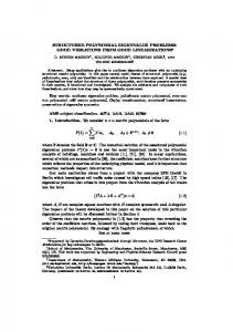
This system has four solutions for (x, y); two real solutions and a complex conjugated pair: (0.08, 2.93), (−4.53, −2.58), and (0.12 ∓ 0.70i, −0.87 ± 0.22i). The system is visualized in Fig. 1.

2.3.2 Preliminary Notions We start by constructing bases of monomials. Let n denote the number of unknowns. In accordance with example Eq. (10)–(11), we consider the case of n = 2 unknowns x and y. Let wδ be a basis of monomials of degree δ in two unknowns x and y, constructed as (12) wδ = (xδ , xδ −1 y, . . . , yδ )T . Given a maximum degree d, a column vector containing a full basis of monomials vd is constructed by stacking bases wδ of degrees δ ≤ d: vd = (w0 ; w1 ; . . . ; wd ).

(13)


5

Fig. 1 A simple set of two polynomials p1 (x, y) = 0 and p2 (x, y) = 0, see Eq. (10) (dot-dashed line) and Eq. (11) (solid line), respectively. This system has four (complex) solutions (x, y): (0.08, 2.93), (−4.53, −2.58), and (0.12 ∓ 0.70i, −0.87 ± 0.22i). Level sets of a polynomial objective function J = x2 + y2 are also shown (dotted lines).

Example 3. For the case of two unknowns x and y, and δ ≤ 3, we have w0 w1 w2 w3

= = = =

(1)T , (x, y)T , (x2 , xy, y2 )T , (x3 , x2 y, xy2 , y3 )T ,

v0 v1 v2 v3

= (1)T , = (1, x, y)T , = (1, x, y, x2 , xy, y2 )T , = (1, x, y, x2 , xy, y2 , x3 , x2 y, xy2 , y3 )T .

(14)

Observe the ‘shift properties’ inherent in this formulation, which will turn out to play a fundamental role in our root-counting technique and root-finding algorithm. By shift properties, we mean that by multiplication with a certain monomial, e.g., x or y, monomials of low degree are mapped to monomials of higher degree. For example: (1, x, y, x2 , xy, y2 )T x = (x, x2 , xy, x3 , x2 y, xy2 )T , (15) (1, x, y, x2 , xy, y2 )T y = (y, xy, y2 , x2 y, xy2 , y3 )T . Let us end with some remarks. Firstly, as the number of unknowns used should be clear in each example, we have dismissed the explicit dependence of vd and wδ on n for notational convenience. Secondly, we have used a specific monomial order, i.e., graded lexicographic order: monomials are first ordered by their total degree, terms of equal total degree are then ordered lexicographically. The techniques illustrated

6


here can be easily generalized to other monomial orders. Thirdly, we have only discussed the case of n = 2 unknowns, however, the general case of n > 2 unknowns can be worked out in a similar fashion.

2.3.3 Constructing Matrices Md We outline an algorithm to construct so-called Macaulay-like matrices Md , satisfying Md vd = 0, where vd is a column vector containing a full basis of monomials, as defined above. This construction will allow us to cast the problem at hand into a linear algebra question. Given a set of m polynomial equations pi , i = 1, 2, . . . , m of degrees di in n unknowns. We will assume that the number of multivariate polynomial equations m equals the number of unknowns n, as this is the case for all the examples we will discuss in this paper. Also recall that only cases with few unknowns are encountered, hence, for notational convenience, unknowns are denoted by x, y, etc. Let d ◦ = max(di ) and let d ≥ d ◦ denote the degree of the full basis of monomials vd to be used. The construction of Md proceeds as follows: The columns of Md index monomials of degrees d or less, i.e., the elements of vd . The rows of Md are found from the forms r · pi , where r is a monomial for which deg(r · pi ) ≤ d. The entries of a row are hence found by writing the coefficients of the corresponding forms r · pi in the appropriate columns. In this way, each row of Md corresponds to one of the input polynomials pi . Example 4. This process is illustrated using Eq. (10)–(11). The 2 × 6 matrix M2 is found from the original set of equations directly as   1 x    3 0 2 1 −1 −1   y2  = 0. M2 v2 = 0 or (16)  5 3 4 1 1 −2  x    xy  y2 We now increase d to d = 3, and add rows to complete M3 , yielding a 6 × 10 matrix. By increasing the degree d to 4, we obtain a 12 × 15 matrix M4 . This process is shown in Tab. 1. In general, the matrices generated in this way are very sparse, and typically quasiToeplitz structured [32]. As d is increased further, the number of monomials in the corresponding bases of monomials vd of the matrices Md grows. The number of monomials of given degree d in n unknowns is given by the relation N(n, d) =

(d + n − 1)! . d! (n − 1)!

(17)


7

Table 1 The construction of matrices Md . Columns of Md are indexed by monomials of degrees d and less. Rows of Md are found from the forms r · pi , where r is a monomial and deg(r · pi ) ≤ d; the entries of each row are found by writing the coefficients of the input polynomials in the appropriate columns. The construction process is shown for d = 2 (resulting in a 2 × 6 matrix), up to d = 4 (resulting in a 12 × 15 matrix). Empty spaces represent zero elements.

d◦

=2

p1 p2 d = 3 x · p1 y · p1 x · p2 y · p2 d = 4 x2 · p1 xy · p1 y2 · p1 x2 · p2 xy · p2 y2 · p2 .. .

1 x y x2 xy y2 x3 x2 y xy2 y3 x4 x3 y x2 y2 xy3 y4 . . . 3 2 1 −1 −1 5 3 4 1 1 −2 3 2 1 −1 −1 3 2 1 −1 −1 5 3 4 1 1 −2 5 3 4 1 1 −2 3 2 1 −1 −1 3 2 1 −1 −1 3 2 1 −1 −1 5 3 4 1 1 −2 5 3 4 1 1 −2 5 3 4 1 1 −2

As d increases, the row-size (number of forms r · pi ) increases too. It can be verified that the number of rows in Md grows faster than the number of monomials in vd , since each input polynomial is multiplied by a set of monomials, the number of which increases according to Eq. (17). Therefore, a degree d ⋆ exists, for which the corresponding matrix Md ⋆ has more rows than columns. It turns out that the number of solutions, and, moreover, the solutions themselves, can be retrieved from the ‘overdetermined’ matrix Md ⋆ , as will be illustrated in the following sections. For the example of Eq. (10)–(11), we find d ⋆ = 6, and a corresponding 30 × 28 matrix M6 . Due to the relatively large size, this matrix is not printed, however, its construction is straightforward, and proceeds as illustrated in Tab. 1. Observe that in Eq. (10)–(11), the given polynomials are both of degree two. If the input polynomials are not of the same degree, one also has to shift the input polynomial(s) of lower degree internally: For example, consider the case of two (univariate) polynomials a 3 x3 + a 2 x2 + a 1 x + a 0 = 0 b2 x2 + b1x + b0 = 0,

(18) (19)

then, for d = 3, one easily finds  1 a0 a1 a2 a3    b0 b1 b2 0   x2  = 0, x  0 b0 b1 b2 x3 





(20)

8


where the third row in the matrix is found by multiplying the second polynomial with x. Increasing d to 4 yields the classical 5 × 5 Sylvester matrix.

2.4 Determining the Number of Roots From the construction we just described, it is easy to verify that the constructed matrices Md are rank-deficient: by evaluating the basis of monomials vd at the (for the moment unknown) roots, a solution for Md vd = 0 is found. By construction, in the null space of the matrices Md , we find vectors vd containing the roots of the set of multivariate polynomial equations. As a matter of fact, every solution generates a different vector vd in the null space of Md . Obviously, when Md is overdetermined, it must become rank deficient because of the vectors vd in the kernel of Md . Contrary to what one might think, the co-rank of Md , i.e., the dimension of the null space, does not provide the number of solutions directly; It represents an upper bound. The reason for this is that certain vectors in the null space are ‘spurious’: they do not contain information on the roots. Based on these notions, we will now work out a root-counting technique: we reason that the exact number of solutions derives from the notion of a truncated co-rank, as will be illustrated in this section. Observe in Tab. 1 that the matrices Md of low degrees are embedded in those of high degree, e.g., M2 occurs as the upper-left block in an appropriately partitioned M3 , M3 in M4 , etc. For Eq. (10)–(11), one has the following situation: d 2(= d ◦ ) 3 4 5 6(= d ⋆ ) 7

w0 × 0 0 0 0 0

w1 × × 0 0 0 0

w2 × × × 0 0 0

w3 0 × × × 0 0

w4 0 0 × × × 0

w5 0 0 0 × × ×

w6 0 0 0 0 × ×

w7 0 0 0 0 0 ×

size Md 2×6 6 × 10 12 × 15 20 × 21 30 × 28 42 × 36

(21)

In the left-most column, the degree d is indicated. The right-most column shows the size of the corresponding matrix Md . The middle part represents the matrix Md . The columns of Md are indexed (block-wise) by bases of monomials wδ . Zeros in Md represent zero-blocks, and blocks of non-zero entries are indicated by ×. For Eq. (10)–(11) we have found that for d ⋆ = 6, the matrix Md ⋆ becomes overdetermined. Let us now investigate what happens to the matrices Md when increasing d. Consider the transition from, say, d = 6 to d = 7. We partition M6 as follows (cf. Eq. (21)):   ××× 0 0 0 0 0 ××× 0 0 0    (22) M6 =   0 0 × × × 0 0  = K6 L6 . 0 0 0 ××× 0 0 0 0 0 ×××


9

where the number of columns in K6 corresponds to the number of monomials in the bases of monomials w0 to w4 . Since M6 is embedded in M7 , we can also identify K6 and L6 in M7 . We partition M7 accordingly:   ××× 0 0 0 0 0 0 ××× 0 0 0 0   0 0 ××× 0 0 0 K6 L6 0   (23) M7 =   = 0 D7 E7 0 0 0 ××× 0 0 0 0 0 0 ××× 0 0 0 0 0 0 ××× Let Z6 and Z7 denote (numerically computed) kernels of M6 and M7 , respectively. The kernels Z6 and Z7 are now partitioned accordingly, such that: T6 M6 Z6 = K6 L6 , and (24) B6 K6 G7 T7 M7 Z7 = , (25) 0 H7 B7 where G7 = L6 0 , H7 = D7 E7 .

and

(26) (27)

Due to the zero block in M7 below K6 , we have rank(T6 ) = rank(T7 ),

(28)

which we will call the truncated co-rank of Md ⋆ . In other words, for d ≥ d ⋆ , the rank of the appropriately truncated bases for the null spaces, stabilizes. We call the rank at which it stabilizes the truncated co-rank of Md . It turns out that the number of solutions corresponds to the truncated co-rank of Md , given that a sufficiently high degree d is chosen, i.e., d ≥ d ⋆ . Correspondingly, we will call the matrices T6 and T7 the truncated kernels, from which the solutions can be retrieved, as explained in the following section.

2.5 Finding the Roots The results from the previous section allow us to find the number of roots as a rank test on the matrices Md and their truncated kernels. We will now present a rootfinding algorithm, inspired by realization theory and the shift property Eq. (15), which reduces to the solution of a generalized eigenvalue problem. We will also point out other approaches to phrase the task at hand as an eigenvalue problem.

10


2.5.1 Realization Theory We will illustrate the approach using the example Eq. (10)–(11). Example 5. A matrix Md of sufficiently high degree was constructed in Section 2.3.3: we found d ⋆ = 6 and constructed M6 . One can verify that the truncated co-rank of M6 is four, hence there are four solutions. Note that one can always construct a canonical form of the (truncated) kernel Vd of Md as follows, e.g., for d = 6 and four different roots:   1 1 1 1  x1 x2 x3 x4     y1 y2 y3 y4   2   x1 x22 x23 x24     x1 y1 x2 y2 x3 y3 x4 y4   2  2 2 2   V6 =  y 1 y 2 y 3 y 4  , (29)  x3 x3 x3 x3  2 3 4   1  x2 y1 x2 y2 x2 y3 x2 y4  2 3 4   1  x1 y2 x2 y2 x3 y2 x4 y2  2 3 4  1  y3 y3 y3 y3  2 3 4   1 .. .. .. .. . . . . where (xi , yi ), i = 1, . . . , 4 represent the four roots of Eq. (10)–(11). Note that the truncated kernels are used to retrieve the roots, this means that certain rows are omitted from the full kernels, in accordance with the specific partitioning discussed in Section 2.4. Observe that the columns of this generalized Vandermonde matrix Vd are nothing more than all roots evaluated in the monomials indexing the columns of Md . Let us recall the shift property Eq. (15): if we multiply the upper part of one of the columns of V6 with x, we have:     1 x  x2  x       y   x =  xy3  . (30) x   x2   2    x y  xy  2 xy2 y Let D = diag(x1 , x2 , x3 , x4 ) be a diagonal matrix with the (for the moment unknown) x-roots. In accordance with the shift property Eq. (15), we can write S1 V6 D = S2 V6 ,

(31)

where S1 and S2 are so-called row selection matrices: S1 V6 selects the first rows of V6 , corresponding to degrees 1 to 5(= 6 − 1). S2 V6 represents rows 2, 4, 5, 7, 8, 9, etc. of V6 , in order to perform the multiplication with x. In general, the kernel Vd is not available in the canonical form as in Eq. (29). Instead, a kernel Zd is calculated numerically as


Md Zd = 0,

11

(32)

where Zd = Vd T, for a certain non-singular matrix T. Hence, S1 Zd (T−1 DT) = S2 Zd ,

(33)

and the root-finding problem is reduced to a generalized eigenvalue problem: (ZTd ST1 S2 Zd )u = λ (ZTd ST1 S1 Zd )u.

(34)

We revisit example Eq. (10)–(11). A kernel of M6 , i.e., Z6 , is computed numerically using a singular value decomposition. The number of solutions was obtained in the previous sections as four. After constructing appropriate selection matrices S1 and S2 , and solving the resulting generalized eigenvalue problem, the roots (x, y) are found as in Example 2.

2.5.2 The Stetter-Möller Eigenvalue Problem It is a well-known fact that the roots of a univariate polynomial correspond to the eigenvalues of the corresponding Frobenius companion matrix (this is how the roots are computed using the roots command in MATLAB). The notion that a set of multivariate polynomial equations can also be reduced to an eigenvalue problem was known to Sylvester and Macaulay already in the late 19th and early 20th century, but was only recently rediscovered by Stetter and coworkers (cf. [1, 31, 39], similar approaches are [19, 21, 30]). We will recall the main ideas from this framework, and illustrate the technique using example Eq. (10)–(11). In order to phrase the problem of solving a set of multivariate polynomial equations as an eigenvalue problem, one needs to construct a monomial basis, prove that it is closed for multiplication with the unknowns for which one searches the roots. Furthermore, one needs to construct associated multiplication matrices (cf. [39, 40]). In practice, this can be accomplished easily after applying a normal form algorithm, such as the Gröbner basis method [3]. Example 6. Consider the example Eq. (10)–(11). It can be verified that (1, x, y, xy)T is closed for multiplication with both x and y, meaning that the monomials x2 , y2 , x2 y, and xy2 can be written as linear functions of (1, x, y, xy)T : From Eq. (10), we find y2 = x2 − xy + 2y + 3. After substitution of y2 in Eq. (11), we find x2 = −1 + 3x + 3xy.

(35)

Multiplication of Eq. (35) with y yields x2 y − 3xy2 = −y + 3xy.

(36)

From Eq. (11), we find x2 = 2y2 − xy − 3x − 4y − 5. After substitution of x2 in Eq. (10), we find y2 = 2 + 2y + 2xy + 3x. (37)

12


Multiplication of Eq. (37) with x yields x2 y − 3xy2 = −y + 3xy.

(38)

We can therefore write Eq. (35)–(38) as    2    x 1 −1 3 0 3 10 0 0  0 1 0 0   y2   2 3 2 2   x         −3 0 −2 1   x2 y  =  0 2 0 2   y  , xy 0 0 −1 3 0 0 1 −3 xy2

(39)

in which the 4 × 4 matrix in the left-hand side of the equation is invertible. This implies    2   x −1 3 0 3 1    y2   2 3 2 2  x ,  2 = (40)  x y   1.8 −6.6 0.2 −7.2   y  0.6 −2.2 0.4 −3.4 xy xy2 from which we easily find the equivalent eigenvalue problems Ax u = x u,

and Ay u = y u,

(41)

or     1 1 0 1 0 0  x   x   0 0 0 1    =   x,   −1 3 0 3  y   y  xy xy 1.8 −6.6 .2 −7.2      1 1 0 0 1 0  x   x   2 3 2 2    =   y,   0 0 0 1  y   y  xy xy .6 −2.2 .4 −3.4 

and

(42)

(43)

from which the solutions (x, y) follow, either from the eigenvalues or the eigenvectors. There are several other interesting properties we can deduce from this example. For example, since Ax and Ay share the same eigenvectors, they commute: Ax Ay = Ay Ax , and therefore also, any polynomial function of Ax and Ay will have the same eigenvectors.

2.6 Finding the Minimizing Root as a Maximal Eigenvalue In many practical cases, and certainly in the polynomial optimization problem we started from in Section 2.2, we are interested in only one specific solution of the set of multivariate polynomials, namely the one that minimizes the polynomial objective function. As the problem is transformed into a (generalized) eigenvalue prob-


13

lem, we can now show that the minimal value of the given polynomial cost criterion corresponds to the maximal eigenvalue of the generalized eigenvalue problem. Example 7. We illustrate this idea using a very simple optimization problem, shown in Fig. 2: min J = x2 + y2

(44)

s. t. y = (x − 1)2 ,

(45)

x, y

the solution of which is found at (x, y) = (0.41, 0.35) with a corresponding cost J = 0.86. The Lagrangian function is given by

Fig. 2 A simple optimization problem, see Eq. (45). The constraint y = (x − 1)2 (solid line) and level sets of J = x2 + y2 (dotted lines) are shown. The solution is found at (x, y) = (0.41, 0.35), for which J = 0.86.

L (x, y, α ) = x2 + y2 + α y − (x − 1)2 .

(46)

The Lagrange multipliers method results in a system of polynomial equations in x, y, and α :

14


∂L (x, y, α ) = 0 ∂x ∂L (x, y, α ) = 0 ∂y ∂L (x, y, α ) = 0 ∂α

⇐⇒

2x − 2xα + 2α = 0,

(47)

⇐⇒

2y + α = 0,

(48)

⇐⇒

y − x2 + 2x − 1 = 0.

(49)

Construct a matrix Md ⋆ as described above. In this example, d ⋆ = 4, for which the dimension of M4 is 40 × 35. The truncated co-rank of Md ⋆ indicates there are three solutions. The corresponding ‘canonical form’ of the (truncated) kernel V4 is given by   1 1 1  x1 x2 x3     y1 y2 y3     α1 α2 α3     x21 x22 x23     x1 y1 x2 y2 x3 y3     x1 α1 x2 α2 x3 α3     y21 y22 y23     y1 α1 y2 α2 y3 α3     α12 α22 α32    3  x32 x33  (50) V4 =  x 1 ,  x2 y1 x2 y2 x2 y3  2 3  21   x α1 x2 α2 x2 α3  2 3  1   x1 y2 x2 y2 x3 y2  2 3  1   x1 y1 α1 x2 y2 α2 x3 y3 α3     x1 α 2 x2 α 2 x3 α 2  1 2 3    y3 y32 y33    1  y2 α1 y2 α2 y2 α3   1  2 3  y α2 y α2 y α2  2 2 3 3   1 1  α3 α23 α33    1 .. .. .. . . . where (xi , yi , αi ) represent the roots (for i = 1, . . . , 3). The objective function is given as J = x2 + y2 . In accordance with the technique described in Section 2.5.1, we now define a diagonal matrix D = diag(x21 + y21 , x22 + y22 , x23 + y23 ) containing the values of the objective function J evaluated at the roots. We have S1 V4 D = S2 V4 ,

or S1 V4 = S2 V4 D−1

(if

J 6= 0),

(51)

Again, S1 and S2 are row-selection matrices. In particular, S1 V4 selects the top rows of V4 , whereas S2 V4 will make a linear combination of the suitable rows of V4 corresponding to the monomials of higher degrees in order to perform the multiplication with the objective function J. Again, the kernel of Md is not directly available in the ‘canonical form’, instead, a kernel is computed as


15

Md Zd = 0,

(52)

where Zd = Vd T, for a certain non-singular matrix T. Hence, S1 Zd = S2 Zd (T−1 D−1 T),

(53)

and the minimal norm is the inverse of the maximal eigenvalue of (S2 Zd )† (S1 Zd )

(= T−1 D−1 T),

(54)

where X† denotes the Moore-Penrose pseudoinverse of X. This leads to the generalized eigenvalue problem (ZTd ST2 S1 Zd )u = λ (ZTd ST2 S2 Zd )u,

(55)

where

1 (56) λ= . J By applying to Zd the right similarity transformation (and a diagonal scaling), we also find Vd . We prefer to work with the power method for computing the maximum eigenvalue, instead of working with the inverse power method for the minimum eigenvalue, since in the inverse power method, a matrix inversion is required in each iteration step. Example 8. We now apply this technique to example Eq. (10)–(11). We want to solve the following optimization problem (also see Fig. 1): min J = x2 + y2

(57)

x,y

s. t. 3 + 2y − xy − y2 + x2 = 0 2

(58) 2

5 + 4y + 3x + xy − 2y + x = 0.

(59)

The method of Lagrange multipliers now results in a set of four polynomial equations in four unknowns. The minimal degree d ⋆ = 5 and corresponding matrix M5 of size 140 × 126 are found as described above. The cost criterion polynomial J is of degree two, which means that S1 V selects the parts of the basis of monomials corresponding to degrees 0 to 3(= 5 − 2). S2 is constructed so that the shift with (x2 + y2 )−1 is performed. The largest real eigenvalue from Eq. (55) yields the minimal cost as 1/0.1157 = 8.64, which is attained at (x, y) = (0.08, 2.93). This can be verified in Fig. 1, where the level sets of the cost function J = x2 + y2 are shown.

16


2.7 Algorithms We have presented a technique to count the roots of systems of polynomial equations. Moreover, the roots can be determined from an eigenvalue problem. Since we search for the maximal eigenvalue of a certain matrix, a possible candidate algorithm is the power method [15]. Current methods for solving sets of polynomial equations can be categorized into symbolic, numerical, and hybrid types. • One can classify symbolic techniques into Gröbner basis methods and resultantbased methods. The work on Gröbner bases [3] has dominated the field of algorithmic algebraic geometry for decades. In this approach, the original problem is transformed into an ‘easier’ equivalent, using symbolic techniques, such as Buchberger’s algorithm [3]. However, Gröbner basis methods have fundamental disadvantages: they are restricted to small-scale problems, and moreover, the computations suffer from numerical instabilities, for example, two problems with seemingly small differences in coefficients can give rise to very differently looking Gröbner bases. Some efforts to bypass the costly generation of a Gröbner basis, by working towards a more direct formulation of a corresponding eigenvalue problem have been made, as in the use of border bases [33, 34]. On the other hand, resultant-based techniques are used to eliminate unknowns from a set of polynomial equations. Resultant-based methods are again gaining interest, as some of the disadvantages of Gröbner basis methods are solved, and the computations involved can be carried out using well-understood matrix computations. • A wide variety of numerical solution techniques based on Newton’s method have been developed. In general, methods based on Newton iterations fail to guarantee globally optimal solutions, but they can be used to find or refine a local solution, starting from an initial guess. Recently, in [20, 36, 38], relaxation methods for the global minimization of a polynomial, involving sums of squares and semidefinite programming have been presented. Many classical methods are often outperformed using this technique. However, in general, only a lower bound of the minimum of the objective function is found. • Hybrid methods combine results from both the symbolic and the numerical perspectives to find all roots. Homotopy continuation methods [23, 43] track all solution paths, starting from an ‘easy’ problem through to the ‘difficult’ problem in question, hereby iterating prediction-correction steps based on Newton methods.

3 Applications in Systems Theory and Identification The tasks of solving polynomial optimization problems and solving sets of polynomial equations are ubiquitous in science and engineering, and a wide variety of applications exists (e.g., computer vision [37], robotics: inverse kinematics [29],


17

computational biology: conformation of molecules [13], life sciences: [2], etc.). The relation between systems theory and system identification, control theory, optimization theory, and algebraic geometry has only come to attention recently [4, 16, 18]. This perspective provides an ambitious and powerful framework to tackle many problems in the fields mentioned above. We highlight some important applications. • The well-known prediction error methods (PEM) [24] can be phrased as optimization problems with a quadratic objective function and polynomial constraints representing the relations between the measured data and the model parameters. This means that they fit into the framework we have proposed above (cf. Section 2.2). The techniques presented here are quite ambitious, as they aim at finding global solutions to polynomial optimization problems. However, at this moment, the inherent complexity prohibits the application to large-scale problems. • Least squares approximation of a matrix by a low-rank matrix is an important task in systems theory and identification, which can be solved using a singular value decomposition [12]. When additional constraints are imposed, e.g., linear matrix structure such as Hankel, or element-wise weighting, the so-called Riemannian singular value decomposition was proposed in [7, 8, 9, 10, 11] to solve the structured total least squares problem. The Riemannian SVD is essentially a system of polynomial equations, and can therefore be tackled using the methods described in this contribution. Moreover, the Riemannian SVD provides a unifying framework [22] for a multitude of existing and new system identification methods, e.g., prediction error methods: AR(X), ARMA(X), dynamical total least squares, errors-in-variables system identification, etc. • In [17] some strong connections between polynomial system solving and multidimensional systems theory were revealed, especially between [40] and realization theory for multidimensional systems. In [16], many other interesting connections between constructive algebra and systems theory are established. • In [26] it was shown that the question of assessing global identifiability for arbitrary (non-linear) model parametrizations is equivalent to the possibility of expressing the model structure as a linear regression: in [25], L. Ljung states: [The] result shows that the complex, non-convex form of the likelihood function with many local minima is not inherent in the model structure.

From the perspective of rearranging the identifiability question as a linear regression, the term ‘algebraic convexification of system identification methods’ was coined. Ljung and Glad use Ritt’s algorithm, based on differential algebra, similar to the Gröbner basis algorithm [3]. Also this approach is related to solving systems of polynomial equations, and can be tackled using the techniques described in this paper.

18


4 Conclusions and Future Work We have explored several fundamental links between systems theory and system identification, optimization theory, and algebraic geometry. We have generalized a technique based on Sylvester and Macaulay resultants, resulting in a method for root-counting as a rank test on the kernel of a Macaulay-like matrix. Also, the solutions can be determined: either as an eigenvalue problem, or by applying realization theory to the kernel of this matrix. In the case of a polynomial optimization problem, this technique can be applied to find the minimizing solution directly, by finding the maximal eigenvalue of a corresponding (generalized) eigenvalue problem. The nature of this contribution is meant to be highly didactic, and presenting main ideas in a pedagogical way. We have omitted proofs and technical details, but yet, many practical challenges remain to be tackled before we can arrive at feasible numerical algorithms: • How to go exactly from the rank deficiency of Md to a (generalized) eigenvalue problem, needs to be investigated further. Moreover, in order to apply the power method, we need to prove that the largest eigenvalue, that is supposed to be equal to the inverse of the minimum of the objective function, is actually real; Said in other words, that there are no complex conjugated roots that in modulus are larger. • Currently, many techniques similar to those described in this paper, suffer from a restrictive exponential complexity due to the rapidly growing number of monomials to be taken into account. This exponential complexity prohibits application to large problems. It remains to be investigated how the inherent complexity can be circumvented by exploiting the (quasi-Toeplitz) structure and sparsity. • The relations between the technique presented here and the traditional symbolic methods will be investigated. The link with the work [14] is relevant in this respect. • How results regarding rank tests, as observed in this article, are encountered in cases where the input polynomials describe a positive dimensional variety is also of interest. • It is not completely clear how some properties observed in the Riemannian SVD framework can be exploited to devise efficient algorithms. For instance, all matrices encountered in this formulation are typically highly structured; It remains to be investigated how these properties might be exploited through the use of FFT-like techniques. Acknowledgements Philippe Dreesen was supported by the Institute for the Promotion of Innovation through Science and Technology in Flanders (IWT-Vlaanderen). Research was also supported by Research Council KUL: GOA AMBioRICS, CoE EF/05/006 Optimization in Engineering (OPTEC), IOF-SCORES4CHEM, several PhD/postdoc & fellow grants; Flemish Government: FWO: PhD/postdoc grants, projects G.0452.04 (new quantum algorithms), G.0499.04 (Statistics), G.0211.05 (Nonlinear), G.0226.06 (cooperative systems and optimization), G.0321.06 (Tensors), G.0302.07 (SVM/Kernel), G.0320.08 (convex MPC), G.0558.08 (Robust MHE), G.0557.08 (Glycemia2), research communities (ICCoS, ANMMM, MLDM); IWT: PhD Grants, McKnow-E,


19

Eureka-Flite+; Helmholtz: viCERP; Belgian Federal Science Policy Office: IUAP P6/04 (DYSCO, Dynamical systems, control and optimization, 2007-2011); EU: ERNSI; Contract Research: AMINAL.

References 1. Auzinger, W., Stetter, H.J.: An elimination algorithm for the computation of all zeros of a system of multivariate polynomial equations. Proc. Int. Conf. Num. Math., pp. 11–30. Birkhäuser (1988) 2. Barnett, M.P.: Computer algebra in the life sciences. ACM SIGSAM Bull. 36, 5–32 (2002) 3. Buchberger, B.: Ein algorithmus zum auffinden der basiselemente des restklassenringes nach einem nulldimensionalen polynomideal. Ph.D. thesis, University of Innsbruck (1965) 4. Buchberger, B.: Gröbner bases and systems theory. Multidimens. Systems Signal Process. 12, 223–251 (2001) 5. Cox, D.A., Little, J.B., O’Shea, D.: Ideals, Varieties and Algorithms. Springer-Verlag (1997) 6. Cox, D.A., Little, J.B., O’Shea, D.: Using Algebraic Geometry, second edn. Springer-Verlag, New York (2005) 7. De Moor, B.: Structured total least squares and L2 approximation problems. Lin. Alg. Appl. 188/189, 163–207 (1993) 8. De Moor, B.: Dynamic total linear least squares. In: Proc. 10th IFAC Symp. System Identif., vol. 3, pp. 159–164. Copenhagen, Denmark (1994) 9. De Moor, B.: Total least squares for affinely structured matrices and the noisy realization problem. IEEE Trans. Signal Process. 42(11), 3104–3113 (1994) 10. De Moor, B.: Linear system identification, structured total least squares and the Riemannian SVD. In: S. Van Huffel (ed.) Recent advances in Total Least Squares Techniques and ErrorsIn-Variables modeling, pp. 225–238. SIAM, Philadelphia (1997) 11. De Moor, B., Roorda, B.: L2 -optimal linear system identification: Structured total least squares for SISO systems. Proc. 33rd Conf. Decis. Control (CDC), Lake Buena Vista, FL (1994) 12. Eckart, G., Young, G.: The approximation of one matrix by another of lower rank. Psychometrika 1, 211–218 (1936) 13. Emiris, I.Z., Mourrain, B.: Computer algebra methods for studying and computing molecular conformations. Algorithmica 25, 372–402 (1999) 14. Faugère, J.C.: A new efficient algorithm for computing Gröbner bases (F4). J. Pure Appl. Algebra 139(1), 61–88 (1999) 15. Golub, G.H., Van Loan, C.F.: Matrix Computations, third edn. Johns Hopkins University Press, Baltimore, MD, USA (1996) 16. Hanzon, B., Hazewinkel, M. (eds.): Constructive Algebra and Systems Theory. Royal Netherlands Academy of Arts and Sciences (2006) 17. Hanzon, B., Hazewinkel, M.: An introduction to constructive algebra and systems theory. In: B. Hanzon, M. Hazewinkel (eds.) Constructive Algebra and Systems Theory, pp. 2–7. Royal Netherlands Academy of Arts and Sciences (2006) 18. Hanzon, B., Jibetean, D.: Global minimization of a multivariate polynomial using matrix methods. J. Glob. Optim. 27, 1–23 (2003) 19. Jónsson, G.F., Vavasis, S.A.: Accurate solution of polynomial equations using Macaulay resultant matrices. Math. Comput. 74(249), 221–262 (2004) 20. Lasserre, J.B.: Global optimization with polynomials and the problem of moments. SIAM J. Optim 11(3), 796–817 (2001) 21. Lazard, D.: Résolution des systèmes d’équations algébriques. Theor. Comput. Sci. 15, 77–110 (1981) 22. Lemmerling, P., De Moor, B.: Misfit versus latency. Automatica 37, 2057–2067 (2001) 23. Li, T.Y.: Numerical solution of multivariate polynomial systems by homotopy continuation methods. Acta Numer. 6, 399–436 (1997)

20


24. Ljung, L.: System identification: theory for the user. Prentice Hall PTR, Upper Saddle River, NJ (1999) 25. Ljung, L.: Perspectives on system identification. Proc. 17th IFAC World Congress, pp. 7172– 7184. Seoul, Korea (2008) 26. Ljung, L., Glad, T.: On global identifiability for arbitrary model parametrizations. Automatica 35(2), 265–276 (1994) 27. Macaulay, F.S.: On some formulae in elimination. Proc. London Math. Soc. 35, 3–27 (1902) 28. Macaulay, F.S.: The algebraic theory of modular systems. Cambridge University Press (1916) 29. Manocha, D.: Algebraic and numeric techniques for modeling and robotics. Ph.D. thesis, Computer Science Division, Department of Electrical Engineering and Computer Science, University of California, Berkeley (1992) 30. Manocha, D.: Solving systems of polynomial equations. IEEE Comput. Graph. Appl. 14(2), 46–55 (1994) 31. Möller, H.M., Stetter, H.J.: Multivariate polynomial equations with multiple zeros solved by matrix eigenproblems. Numer. Math. 70, 311–329 (1995) 32. Mourrain, B.: Computing the isolated roots by matrix methods. J. Symb. Comput. 26, 715–738 (1998) 33. Mourrain, B.: A new criterion for normal form algorithms. In: Applied Algebra, Algebraic Algorithms and Error-Correcting Codes, Lecture Notes in Computer Science, vol. 1710, pp. 430–443. Springer, Berlin (1999) 34. Mourrain, B., Trébuchet, P.: Solving complete intersections faster. Proc. ISSAC 2000, pp. 231–238. ACM, New York (2000) 35. Nocedal, J., Wright, S.J.: Numerical Optimization, second edn. Springer (2006) 36. Parrilo, P.A.: Structured semidefinite programs and semialgebraic geometry methods in robustness and optimization. Ph.D. thesis, California Institute of Technology (2000) 37. Petitjean, S.: Algebraic geometry and computer vision: Polynomial systems, real and complex roots. J. Math. Imaging Vis. 10, 191–220 (1999) 38. Shor, N.Z.: Class of global minimum bounds of polynomial functions. Cybernetics 23(6), 731–734 (1987) 39. Stetter, H.J.: Matrix eigenproblems are at the heart of polynomial system solving. ACM SIGSAM Bull. 30(4), 22–25 (1996) 40. Stetter, H.J.: Numerical Polynomial Algebra. SIAM (2004) 41. Stetter, H.J.: An introduction to the numerical analysis of multivariate polynomial systems. In: B. Hanzon, M. Hazewinkel (eds.) Constructive Algebra and Systems Theory, pp. 35–47. Royal Netherlands Academy of Arts and Sciences (2006) 42. Sylvester, J.J.: On a theory of syzygetic relations of two rational integral functions, comprising an application to the theory of sturms function and that of the greatest algebraical common measure. Trans. Roy. Soc. Lond. (1853) 43. Verschelde, J., Verlinden, J., Cools, R.: Homotopies exploiting Newton polytopes for solving sparse polynomial systems. SIAM J. Numer. Anal. 31, 915–930 (1994)

Index

algebraic geometry, 2, 16–18 applications, 1, 2, 16, 17

power method, 2, 15, 16, 18 prediction error methods, 2, 17

control theory, 17

quasi-Toeplitz structure, 6, 18

eigenvalue decomposition, 2, 3, 9, 11, 12, 15, 16, 18 errors-in-variables, 17

realization theory, 2, 9, 17, 18 resultant, 16, 18 Riemannian singular value decomposition, 17, 18 root-counting, 2, 5, 8, 9, 16, 18 root-finding, 2, 5, 7, 9–11

first-order conditions, 3 global identifiability, 17 Gröbner basis, 11, 16, 17

optimization theory, 2, 17, 18

singular value decomposition, 11, 17 solving sets of polynomial equations, 3, 4, 11, 16, 17 sparsity, 6, 18 structured total least squares, 2, 17 Sylvester, 2, 8, 11, 18 system identification, 2, 17, 18 systems theory, 2, 17, 18

polynomial optimization problem, 1–3, 12, 16–18

truncated co-rank, 8–10, 14 truncated kernel, 9, 10, 14

Lagrange multipliers, 1–3, 13, 15 linear algebra, 2, 4, 6 Macaulay, 2, 11, 18

21