Jan 14, 1997 - tions; Measurement Error; Nonlinear Regression; Nutrition. ... The polynomial regression model under multiplicative measurement is given by.
POLYNOMIAL REGRESSION AND ESTIMATING FUNCTIONS IN THE PRESENCE OF MULTIPLICATIVE MEASUREMENT ERROR, WITH APPLICATIONS TO NUTRITION Stephen J. Iturria, Raymond J. Carroll and David Firth � January 14, 1997
Abstract
In this paper we consider the polynomial regression model in the presence of multiplicative measurement error in the predictor. Consistent parameter estimates and their associated standard errors are derived. Two general methods are considered, with the methods di�ering in their assumptions about the distributions of the predictor and the measurement errors. Data from a nutrition study are analyzed using the methods. Finally, the results from a simulation study are presented and the performances of the methods compared.
Key Words and Phrases: Asymptotic theory; Bootstrap; Errors-in-Variables; Estimating Equations; Measurement Error; Nonlinear Regression; Nutrition. Short title: Multiplicative Measurement Error
Stephen Iturria is a graduate student and Raymond J. Carroll is Professor of Statistics, Nutrition and Toxicology, Department of Statistics, Texas A&M University, College Station, TX 77843{3143. David Firth is Senior Fellow in Statistics for the Social Sciences, Nu�eld College, Oxford OX1 1NF. The authors wish to thank Suojin Wang for his generous and helpful comments during the preparation of this article. Iturria and Carroll's research was supported by a grant from the National Cancer Institute (CA{57030). Carroll's research was partially completed while visiting the Institut fur Statistik und Okonometrie, Sonderforschungsbereich 373, Humboldt Universitat zu Berlin, with partial support from a senior Alexander von Humboldt Foundation research award. �
1 INTRODUCTION Much work has been done in the estimation of regression coe�cients in the presence of additive measurement error in the predictors. A detailed account of the developments for linear regression models can be found in Fuller (1987). Carroll, et al. (1995) summarize much of the recent work for nonlinear regression models. Considerably less work has been done for cases of nonadditive measurement error however. Hwang (1986) derives a consistent estimator for the coe�cients of the ordinary linear model under multiplicative measurement error by modifying the usual normal equations of least squares regression. To apply this method, one requires consistent estimates of the moments of the measurement errors. One of the general methods we will consider is a special case of Hwang's estimator. For this method we do not require that any distributional assumptions be made about the unobserved predictor, other than the usual i.i.d. assumptions. We will consider two distributional forms for the measurement errors, and propose methods for estimating their moments. For the second general method we will consider, we model the distribution of the unobserved predictor as well. Fitting this method will require estimating the distribution of the predictor conditional on its mismeasured version. We will apply our methods to a nutrition data set taken from the Nurses Health Survey. We also present the results from a simulation study.
1.1 The Polynomial Regression Model The polynomial regression model under multiplicative measurement is given by
Yi = 0 +
p X k=1
k Xik + pt +1 Zi + �i ;
Wij = Xi Uij ; i = 1; : : : ; n; j = 1; : : : ; ri ; where Uij is the measurement error associated with the j th replicate of the error{prone predictor of Xi , namely Wij , and Zi is a vector of covariates assumed to be measured without error. Further assumptions are that all elements of (�i ), (Uij ), and (Xi ) are mutually independent, the (Xi ) assume positive values only, the (�i ) have mean zero, and the (Uij ) have either mean or median one. We will consider three possible models for the distribution of the (Xi ; Uij ). No further distributional assumptions will be made about the (Zi ) and (�i ).
1
OLS fit for Energy Vs. Vitamin A •
• •
2.5 •
•
• •
• •
• •
•
• •
•
•
2.0
• •
• • •
• •
• ••
Average Energy
•
•
• •
•
• • •
•
•
• •• • • • •• • • • • • • • • • • • • • • • • • • • • •• • • • • • • • • • • •• • • • • • • • • •• • • •• • • • •• • • • • • • • • • • • • • • • • • • • ••• • • • • • • • • • • • • • • • • • • • • • • • • • •
•
• •
•
1.5
•
• • •
•
• •
•
• •
• •
•
•• •
1.0
••
2
•
4
6
8
10
12
Average Vitamin A
Figure 1: Least squares quadratic t for Nurses.
1.2 Nurses Health Survey The Nurses Health Survey includes measurements of energy intake and vitamin A intake for 168 individuals calculated from four 7{day food diaries. We will model Y = long{term energy intake as a quadratic function of X = long{term vitamin A intake plus error. No important e�ects were evident among the possible covariates so we will only consider the regression of Y on X . Food diaries are an imprecise method for calculating long{term nutrient intakes so the reported vitamin A intakes are presumed to be measured with error. Long{term energy intake is also estimated imprecisely when using food diaries, but for the purpose of illustrating our methods we will take such measurement errors to be additive, thus absorbing them into the (�i ). A scatter plot of the averages of the energy replicates against the averages of the vitamin A replicates is given in Figure 1. The p{value for the quadratic term in the ordinary least squares (OLS) t of the energy replicate averages as a quadratic function of the vitamin A replicate averages is :002.
1.3 E�ects of Multiplicative Measurement Error on Curvature One question to consider is whether the curvature exhibited in the OLS t of the Nurses data accurately re ects the curvature in the underlying relationship between Y and the unobservable X . To see the e�ect that measurement error can have on curvature, consider the plots given in Figure 2. The top two plots are of Y vs. X and Y vs. W for data generated from a linear regression model with right{skewed, multiplicative measurement errors. Note the curvature exhibited in the plot of 2
(a) • •
5
2 1
5
2.5
Y
2.0
1.5
1.0
10
4
Y
3
3 2 1
True
• • • • • • • •• • • • • ••••• • • • ••• • • •• • •• • •• • • • •• • • • •• • • • ••• • ••• •• • • • •••• • • • • • • • • • • • ••• • • • •• • • ••• • •• ••• • • • • • • • • • •• •• • • • • • • • •• • • • • • • • • •• • • •• • •• • • •• • • • •• ••• •• ••• • • • • • • • • • • • ••• • • • • • • • • • • •• •
•
•
OLS True
• •
15
5
10
15
X
(W1+W2)/2
(c)
(d)
• • • • •••• •• • • • • ••• •• • •• ••• • ••• • • • • ••• • • • • • • • •• • • • ••• • •• • • • • • •• • • • • • • ••••• ••• • • •••• • • • • • • •• •• • ••• •• • • ••• • •• • • • • • •• • • • • • •• • • •• • • • • •• • •• •• ••• • • •• • •• •• •• • •• • •• • • • • ••• • •• •• • • • • •• • • •• • • • • •
2.5
2.0
1.5
1.0
• 0.5
•
5
• • • • • •• ••• • • • • • • • •• • • • • • • • • • • •••• ••• •• ••• •• • • ••• • • •• • • • • •• • • • • •• • • • • • •• • • • • • • • ••• •• • • •• • • • • • •• • • • • • • • • • • • • • • • •• • • • • • • • • • • • • • • • • • • • • • • • • • • • • • • • ••• •• ••• •••• •• • •• ••• • •
Y
Y
4
(b)
• • • • •• • ••• • • • • •• •• •••• •• • •• • • • •• • •• • • • •• • •• • • • • • ••• •• •••• • • • • •• • • •• •• • ••• • •• • •• • • • ••• •• ••• • ••• •• • • • • • •• • • •• ••• • • • • •• • • • • ••• • • • ••••• • • • • • • • ••••• •• ••• • • •• •• ••• • •• ••• • • •• • • • • •• • • •
• • •
•
•
•
• True
0.5
• 5
10
15
OLS True
• 5
X
10
15
(W1+W2)/2
Figure 2: Plots for two simulated data sets: (a) Y vs X for linear model, (b) Y vs W for linear model, (c) Y vs X for quadratic model, (d) Y vs W for quadratic model.
Y vs. W . Measurement errors of this type can also have the e�ect of dampening the curvature of
the underlying model. The second pair of plots are for data generated from a quadratic regression model with 2 < 0. The common feature of the two pairs of plots is that the measurement errors tend to \stretch" the data along the X {axis, giving a distorted view of the true relationship between Y and X .
1.4 Diagnostics for Multiplicative Measurement Error Measurement error models have been most fully developed for the additive error case, W = X + U , with U being either a mean{ or median{zero error term that is independent of X . A convenient diagnostic for assessing additivity when X is independent of the mean{zero measurement error term are plots of jWij ? Wik j against Wij + Wik for various j 6= k, where Wij is the j th replicate for individual i. In the appendix we show that under the additive model, one would expect to see no correlation in these plots. If, however, the multiplicative model, W = XU , is more appropriate, then an additive error model is appropriate when considering the logarithm of W . Plots of jlog(Wij ) ? log(Wik )j against log(Wij ) + log(Wik ) therefore provide a ready diagnostic for multiplicative measurement error. For our analysis of the Nurses data we will de ne Yi to be the average of the four energy replicates for individual i, Wi1 to be the average of the rst two vitamin A replicates for individual i, and Wi2 to be the average of the third and fourth vitamin A replicates for individual i. The 3
|log(W1) - log(W2)| vs. log(W1) + log(W2)
|W1 - W2| vs. W1 + W2
•
•
8 •
1.0
•
•
•
• •
•
• •
0.8
0.6
• •
•
• ••
• • 0.4
• •
0.2
• •
•
0.0 1
•
•
• • • •
•
•
•
•
• •
3
•
4
4
• •
0 5
•
•
•
•
• •
• • •
5
•
• •
• •
•
•
• • • •• • • • • • • • ••• • • ••• • • •• • • •• • • • • • • • • • ••• • • • •• •• •• •• • • ••• •• • ••• • • • • •• •• • • •• • • •• • ••• • •• • •• • • • • • • •••• •• • • • • • •• • • ••
10
•
• •
• • • • • • • • ••
••
2
log(W1) + log(W2)
•
•
•
• • • • • • • • •• • • •• ••• • •• • • • • • • • • •• • •• • • • •• •• • • • • • • • • • • •• •• • • • • • • •• • • • • • • • •• •• • • • • • •• •• • • • • • • • • • • •• • • • • • • • • •• • • • • • • • • •• • ••
2
• • •
•
•
•
•
• •
•
|W1 - W2|
|log(W1) - log(W2)|
•
6
•
• • • • • •• •
• • •••
15
• •
•
20
25
W1 + W2
Figure 3: Measurement error diagnostics for Nurses data. diagnostics for the Nurses data are given in Figure 3. The correlation coe�cient for the plot of jlog(Wi1 ) ? log(Wi2 )j against log(Wi1 ) + log(Wi2 ) is ?:02, suggesting that the measurement errors are additive in the log{scale, and hence multiplicative in the untransformed scale. To see that an additive model is not appropriate for the data in the original scale, note the strength of the correlation in the plot for the untransformed data, which has a corresponding correlation coe�cient of :50.
1.5 Models for (
X; U
)
We will consider two distributional forms for the measurment error, U . The rst form is where U can be expressed as exp(V ), where V is mean-zero and symmetric. The second form is a special case of the rst, that U is lognormal(0,�u2 ). Note that in both cases we have that W is median{unbiased for X . (The assumption of median as opposed to mean unbiasedness is not really important since there is no way to distinguish between the two cases in practice. The advantage to assuming median{unbiasedness in the case of lognormal measurement error is that it simpli es the identi cation of parameters.) When working with the rst distributional form for U , we do not place any distributional assumptions on X other than that X is nonnegative with nite moments. We call this the nonparametric case. For the second distributional form of U , the case of lognormal measurement error, we consider two possibilities for X . The rst is where once again we assume only that X is nonnegative with nite moments, which we call the semiparametric case. The second form is that X , conditional on Z , is distributed lognormal(�0 + �t1 Z ,�x2 ), which we will call the 4
Table 1: Three estimation scenarios. Model Nonparametric Semiparametric Parametric
X jZ
U
exp(V ), V mean-zero symmetric nonnegative 2 nonnegative lognormal(0,�u ) lognormal(�0 + �t1 Z ,�x2 ) lognormal(0,�u2 )
parametric case. The three scenarios are summarized in Table 1. Note that the semiparametric model is a special case of the nonparametric model, and that the parametric model is a special case of the other two models. Also note that these names refer only to the assumptions placed on the X and U . For example, the parametric model is not fully \parametric" in that we do not assume anything beyond independence and a zero expectation for the (�i ). We believe this is one of the attractive features of our method.
1.6 Unbiased Estimating Functions for Polynomial Regression under Multiplicative Measurement Error We derive consistent estimators for the coe�cients of the polynomial regression model using the theory of estimating equations. An advantage to formulating estimators in terms of estimating equations is that the theory provides a general method for computing asymptotic standard errors. A brief overview of the method is provided in the appendix. A more detailed description can be found in Carroll, et al. (1995). In practice, the estimating function, (�), is not formulated independently, but rather is a consequence of the estimation method being considered. For example, a maximum likelihood approach would imply taking (�) to be the derivative of the log{likelihood. Note that for the polynomial regression model, an unbiased estimating function for B = ( 0 ; pt +1 ; 1 ; : : : ; p )t when the distribution of U is known is
0 (Y ? ? t Z ? Pp W k =c )(1; Z t )t BB (Y ? ? t p Z )W=c ? kPp Wk k =c k k p (Y; W; Z; B) = B @ �p � � Pp k p (Y ? ? pt Z )W =cp ? k W =ck 0
0
0
+1
+1
1
1
+1
1
+
+1
1
+1
1 CC CA ;
p
+
where W is the average of the replicates of W , and ck is the kth moment of U . In practice, the distribution of U will be unknown and the ck will have to be estimated. Unbiased estimating functions for the nonparametric and semiparametric cases can be found by modifying (�) to incorporate the estimation of the ck . We take up methods for estimating the ck in the next section. 5
For the parametric case, we take an alternative approach that allows us to exploit our knowledge P of the distributional form of X . De ning Ti = ri ?1 r1i log(Wij ), i = 1; : : : ; n, and noting that E (Y jT; Z ) = 0 + pt +1 Z +Pp1 k E (X k jT; Z ), a method for estimating B is to regress the Yi on the Zi and on estimates of the E (X k jTi ; Zi ). Simple calculations give us that the conditional distribution of X given (T; Z ) is lognormal with parameters (�u2 �xjz + 2�x2 T )=(�u2 + 2�x2 ) and �x2 �u2 =(�u2 + 2�x2 ), where �xjz = �0 + �t1 Z . The exact form of the unbiased estimating equation for the parametric case is given in the next section.
2 ANALYSIS OF MEASUREMENT ERROR
2.1 Error Parameter Estimation
Computing estimates of the E (U k ) in the nonparametric and semiparametric cases requires that we obtain estimates for the moments of U . Let mk denote the kth moment of U . An estimator for h i1=2 mk in the nonparametric case is given by mb k = Pn1 Prji6=l fnri(ri ? 1)g?1 (Wij =Wil )k , which h n oi1=2 follows from the fact that E (Wij =Wil )k = mk , for all i; j; k; l. For the semiparametric and parametric models, in which U is lognormal(0,�u2 ), we can take �bu2 to be the mean-square error resulting from an ANOVA on the log(Wij ), which is unbiased for �u2 . Since the kth moment of lognormal(0,�u2 ) is exp(k2 �u2 =2), an estimator for mk in the semiparametric case is then given by mb k = exp(k2 �bu2 =2). Moments of U for the nonparametric and semiparametric cases can be estimated by substituting the mb k into the expansions of the E (U k ). For the parametric model, in addition to �bu2 , we need estimators for �0 , �1 , and �x2 . Estimates for �0 and �1 are given by the regression of the log(Wij ) on the Zi . By the independence of X and U , an unbiased estimate for �x2 is given by �bx2 = ?�bu2 + Pn1 Pr1i (nri )?1 flog(Wij ) ? �b0 ? �bt1 Zi g2 .
2.2 Unbiased Estimating Equations for the case of two replicates An unbiased estimating function for the nonparametric estimator when ri = 2, i = 1; : : : ; n, is given by
0 t Z ? Pp k W k =ck )(1; Z t )t ( Y ? ? p BB P BB (Y ? ? pt Z )W=c ? p k W k =ck ��� B NP (Y; W; Z; BNP ) = B BB (Y ? ? pt Z )W p=cp ? Pp k W k p=ck BB ?m + f(W =W ) + (W =W )g B@ ��� p n o ?m p + (W =W ) + (W =W ) p 0
+1
0
1
+1
+1
1
+
0
+1 1 2
2 1
2 2
1
1 2
6
1
1
1
2
2
2
2
2
1
1
2
1 CC CC CC pC CC ; CC A
+1
+
where BNP = ( 0 ; pt +1 ; 1 ; : : : ; p ; m21 ; : : : ; m22p )t , with the ck treated as functions of the m2k . For the semiparametric estimator, an unbiased estimating function is
0 P (Y ? ? pt Z ? p k W k =ck )(1; Z t )t BB P (Y ? ? pt Z )W=c ? p k W k =ck B SP (Y; W; Z; BSP ) = B ��� BB @ (Y ? ? pt Z )W p=cp ? Pp k W k p=ck ?2�u + flog(W ) ? log(W )g 0
+1
0
1
+1
1
+1
+1
1
+
0
+1
1
2
1
where BSP = ( 0 ; pt +1 ; 1 ; : : : ; p ; �u2 )t , with the ck
+
2
2
1 CC CC ; CC pA
treated as functions of �u2 . Finally, an unbiased estimating function in the parametric case is given by
P v )(1; Z t )t 1 0 (Y ? ? pt Z ? p P k k p t BB CC (Y ? ? p Z )v ? k vk v CC BB � � � Pp CC ; B t CM (Y ? ? p Z )vp ? k v k vp (Y; W; Z; BCM ) = B �log(W BB CC ) + log(W ) ? 2� ? 2�� t Z (1; Z t )t B@ C � ?2�x ? 2�u + log(W ) ? � ? �t Z + log(W ) ? � ? �t Z A ?2�u + flog(W ) ? log(W )g where we de ne vk = E (X k jT; Z ), and BCM = ( ; pt ; ; : : : ; p ; � ; � ; �x ; �u )t . We will call the 0
+1
+1
0
+1
1
2
1
0
1
1
2
2
1 2
0
0
0
1
2
1
1
+1
1
1
1
2
0
1
2
2
2
0
2
1
2
solution to this estimating equation the conditional mean estimator, in reference to the conditioning on T and Z . We prefer this name over \parametric" estimator since the latter suggests a likelihood{ based estimator. Note that a likelihood estimator would require assuming a distributional form for �, something we wish to avoid.
2.3 Asymptotic Variance Comparisons Asymptotic variances for the estimators are found by taking one{term Taylor series approximations of (�) at the estimates, Bb. An outline of the derivations for the case of quadratic regression without covariates is given in the appendix. The variances are calculated under the assumptions of the parametric model, with the additional assumption of nite and constant variance for the (�i ). We can use these formulae to calculate the asymptotic relative e�ciency (ARE) of the conditional mean estimator relative to both the nonparametric and semiparametric estimators for various parameter values. This allows us to assess the gain in e�ciency that results from choosing to model X when the parametric model holds. Plots of the AREs for b2 are shown in Figure 4. The AREs were computed using the parameter estimates for the Nurses data given in the next section, except that �u2 was allowed to vary, and are plotted as a function of the ratio of the coe�cients of variation for U and X . This allows us to see how the e�ciency of the conditional mean estimator varies with changes in the 7
ARE of the C.M. estimator vs. C.V.(U)/C.V.(X) for Nurses 7
6
5
ARE
C.M. vs. Semipar. C.M. vs. Nonpar. 4
3
2
1
0.0
0.2
0.4
0.6
0.8
1.0
C.V.(U)/C.V.(X)
Figure 4: ARE of C.M. estimator vs. C.V.(U)/C.V.(X) for Nurses. relative amount of measurement error. The plot is consistent with our simulation studies in that under the parametric model, the nonparametric and semiparametric methods produce virtually identical estimates for large n. More results from our simulation study are given later.
3 NUMERICAL EXAMPLE
3.1 Diagnostics for and U
X
for the Nurses Data
In order to determine which of the three methods is the most appropriate for the Nurses data, we must characterize the distributions of U and X . We can assess the lognormality of U by constructing the Q{Q plot for log(Wi1 =Wi2 ), i = 1; : : : ; n. If U is lognormal, this plot should look like that for normally distributed data. If the lognormality assumption for U is valid, a diagnostic for lognormality of X is the Q{Q plot for log(Wi1 ) + log(Wi2 ), i = 1; : : : ; n. For lognormal X , this plot should also look like a Q{Q plot of normally distributed data. Examination of these plots in Figure 5 suggests that the lognormality assumption is reasonable for both X and U . Taken together, the above diagnostics suggest that the conditional mean estimator is reasonable for the Nurses data.
3.2 Regression Fits for the Nurses Data Plots of the tted regression functions are given in Figure 6. We computed 95% con dence intervals for the estimates of 2 using bootstrap percentiles. Con dence intervals for the NP, SP, CM, and 8
QQ-plot for log(W1/W2) for Nurses
QQ-plot for log(W1)+log(W2) for Nurses •
•
5
•
1.0
• •• •
•• • • ••• •••• •• ••••• •• ••••••• •• • • • ••••• ••• •••• •• •••• ••• • ••• ••• •••• •••• ••••• ••••• • ••••• ••••• •••• •••• ••••••• • • • • • • ••• • • •••• • ••
•
0.0
-0.5
••
4
log(W1)+log(W2) quantiles
log(W1/W2) quantiles
0.5
•• • • • • •••• •••• ••• •• ••••• • • • • • •••• •••• ••••• •• •••• •••• • • • ••• •••••• •• •••• •••• • • ••• ••• ••• ••• ••••• • • • • •••••• •• •••• ••• •••• • •• •• •• ••
3
2
•
•
••
• •
• • -1.0
••
•
•
•
1
•
•
-2
-1
0
1
2
-2
z quantiles
-1
0
1
2
z quantiles
Figure 5: Q{Q plots for log(W1/W2) and log(W1)+log(W2) for the Nurses data. OLS estimators respectively were: (-.121,-.014), (-.165,-.015), (-.051,-.014), and (-.022,-.006). Our simulation results demonstrated that bootstrap percentiles provided the most reliable intervals.
4 SIMULATION STUDY
4.1 Overview
A simulation study was carried out to assess the relative performance of the three methods under the parametric model without covariates. Generating parameter values were taken from the t of the conditional mean estimator for the Nurses data. Parameter values used were B = (:464; :398; ?:029)t , �x = 1:613, �x2 = :094, and �u2 = :076. The (�i ) were taken to be i.i.d. N(0,��2 ), with ��2 = :101 being the mean of the squared deviations of the data about the conditional mean t.
4.2 Some Descriptive Statistics Given in Table 2 are the medians, MADs, and estimated root mean square errors of b2 for 5000 simulated data sets. The sampling distributions for the nonparametric and semiparametric estimators, although asymptotically normal, were found to be highly skewed for n = 168, making necessary the use of the more robust medians and MADs to assess the bias and standard errors. As one might expect, the OLS estimates were the least variable, but were also the most biased. We see that the conditional mean estimator provided the most favorable tradeo� between bias and 9
Energy vs. Vitamin A •
• •
2.5
• •
•
• • •
•
2.0
• • •
• • •
NP SP CM OLS
•
•
•
• ••
• •
••
• •
•
• • •
•
• •
•
• • • • • • •• • • • • • • •• • •• ••• • •• • • • • • • •• • • •• •• • • • • • • • • • • • • • • • •• • • • • • • • • • •• • • • • • • • • • • • • • • • • • • • ••• • • • • • •• • • • • • • • • • •• • • • • • • • •
•
• •
Energy
•
1.5
• • •
1.0
•
•
• • •
•
•
• ••
0.5
0
5
10
15
Vitamin A
Figure 6: Nonparametric, semiparametric, conditional mean, and OLS ts for the Nurses data. Table 2: Summary statistics for b2 , 2 = ?:029. NP SP CM OLS
median -0.035 -0.036 -0.028 -0.012
MAD sqrt(MSE) 0.018 .019 0.020 .021 0.010 .013 0.004 .016
variance reduction. It is important to note that the nonparametric and semiparametric models both contain the parametric model as a special case, and so are not \incorrect" models for the simulated data. What is evident, however, is that there may be considerable gains to be made if one is willing to model the distribution of the predictor, X .
4.3 Bootstrap{Percentile Con dence Interval Widths and Coverages The performances of 95% bootstrap{percentile con dence intervals for 2 were examined by generating 500 data sets at the Nurses parameter estimates and computing bootstrap intervals based on 1000 with{replacement samples. Empirical coverage probabilities and mean con dence interval lengths for the 500 intervals are given in Table 3. We see that only the con dence intervals for the conditional mean estimator provided both accurate coverage and reasonable length. Further simulations showed that as sample size increases, the performances of the nonparametric and 10
Table 3: Simulated bootstrap con dence interval coverages and mean lengths, n = 168. Coverage Mean length
NP SP CM OLS .960 .976 .942 .182 .470 .663 .051 .020
semiparametric estimators approach that of the conditional mean estimator. Much of the poor performance of the nonparametric and semiparametric methods at moderate values of n appears to be due to highly skewed sampling distributions for the estimators at those sample sizes.
5 GENERALIZATIONS The methods and results of this paper are easily extended to general estimating functions. In the additive error case, a series of works by Stefanski (1989), Nakamura (1990), Carroll, et al. (1995), and Buzas & Stefanski (1996) have established the method of corrected estimating equations. Under various guises, the basic idea is that in some cases, an estimating function (Y; X; Z; B) can be expanded as a polynomial (Y; X; Z; B) =
1 X
j =0
j (Y; Z; B)X j :
For the special structure of the additive model, expansions can be done either in powers of X as above, powers of exp(X ), or combinations of the two. For the multiplicative model, expanding in powers of X is most convenient. Note that this is equivalent to rst replacing X by its logarithm X� , thus obtaining an additive model, and then expanding the estimating function in terms of powers of exponentials of X� . For the multiplicative model, if the moments of U are known then under appropriate regularity conditions relating to convergence of the sum, an unbiased estimating function for B is
X UB (Y; W; Z; B) = j (Y; Z; B)W j =cj ; j =0 1
where cj is the j th moment of U . For instance, it is easily seen that for the polynomial regression model, the estimating equations for the nonparametric and semiparametric estimators are of this form up to the nuisance parameters (m1 ; : : : ; m2p )t and �u2 respectively, where mk = E (U k ). The general equivalent of the parametric approach is described brie y as follows. Suppose that 11
we can expand both the mean and variance of Y in powers of X , so that
E (Y jX; Z; B) =
1 X
j =0
dj (Z; B)X j ;
1 X
ej (Z; B)X j ;
(1)
di(Z; B)dj (Z; B)(vi+j ? vi vj );
(2)
var(Y jX; Z; B) =
j =0
Then provided that the following sums converge, we have
E (Y jW; Z; B) = var(Y jW; Z; B) =
1 X j =0
ej (Z; B)vj +
1 X
j =0
dj (Z; B)vj ;
1X 1 X i=0 j =0
where vj = E (X j jW; Z ). If we assume a parametric distribution for X and U , the vj are known up to parameters and we can estimate B via ordinary quasilikelihood (generalized least squares). In our formulation of the conditional mean estimator for polynomial regression, we did not specify a model for var(Y jX; Z; B), but rather worked only with E (Y jX; Z; B). Since we are not directly specifying a variance model, for the purposes of estimation we have computed the ordinary least squares estimate of B, given estimates of the vj . This is in e�ect a solution to a generalized estimating equation with a homoscedastic \working" variance function (Zeger, et al., 1988). Modeling the variance of Y given (X; Z ) as in (1) and using (2) as the observed variance function may lead to a more e�cient estimator, but as seen in Figure 4, our working parametric solution is already reasonably e�cient relative to the nonparametric and semiparametric estimators. We do wish to reemphasize, however, that the gains in e�ciency come from correctly modeling the distribution of X .
CONCLUDING REMARKS In this paper we have considered two general approaches to tting polynomial regression models in the presence of multiplicative measurement error in the predictor. The approaches di�ered in that for one we did not make any distributional assumptions for the predictor beyond the usual i.i.d. assumption, and for the other we assumed a distributional form. In our analysis we found that the latter approach, though less robust, can in some cases lead to a substantial increase in e�ciency, particularly for small to moderate sample sizes. We also found that these gains in e�ciency increase with the degree of the measurement error. Much of the gain in e�ciency appears due to the slow convergence to normality of the less parametric approach.
REFERENCES 12
Buzas, J. S. & Stefanski, L. A. (1996). A note on corrected score estimation. Statistics & Probability Letters, 28, 1{8. Carroll, R. J., Ruppert, D. and Stefanski, L. A. (1995), Measurement Error in Nonlinear Models. London: Chapman and Hall. Hwang, J. T. (1986). Multiplicative errors in variables models with applications to the recent data released by the U.S. Department of Energy. Journal of the American Statistical Association, 81, 680-688. Fuller, W. A. (1987). Measurement Error Models. John Wiley and Sons, New York. Nakamura, T. (1990). Corrected score function for errors-in-variables models: Methodology and application to generalized linear models. Biometrika, 77, 1, 113-116. Stefanski, L. A. (1989). Unbiased estimation of a nonlinear function of a normal mean with application to measurement error models. Communications in Statistics, Series A, 18, 4335{4358. Zeger, S. L., Liang, K. and Albert, P. S. (1988). Models for longitudinal data: A generalized estimating equation approach. Biometrics, 44, 1049{1060.
6 APPENDIX
6.1 Justi cations for the Measurement Error Diagnostics
R R
1 1 js ? For the additive model, Cov(jW1 ? W2 j; W1 + W2 ) = E fjU1R ? UR2 j(U1 + U2 )g, which is ?1 ?1 1 1 js + rj(s ? r)f (s)f (r) ds dr, tj(s + t)fU1 (s)fU2 (t) ds dt. By a change of variable, this is ?1 U U 1 2 ?1 which is 0. Similarly, for the multiplicative model, Cov fjlog(W1 ) ? log(W2 )j; log(W1 ) + log(W2 )g is 0.
6.2 Estimating Functions
A function (Y; X; B) is an unbiased estimating function for B if E f (PY; X; B)g = 0. Given such a function, (�), one possible estimator for B is the solution, Bb, of n?1 n1 (Yi ; Xi ; B) = 0. Under a set of mild regularity conditions on , one can show that Bb is a consistent estimator of B. The limiting distribution of Bb can be found by taking a rst-order Taylor series approximation P n ? 1 b of n 1 (Yi ; Xi ; B ) about B , and then applying Slutsky's Theorem and the CLT. One nds � that asymptotically n1=2 (Bb ? B ) has mean 0 and covariance A?1 BA?t , where A = E (@=@ Bt ) , � B = E (Y; X; B) t (Y; X; B) , and A?t = (A?1 )t .
6.3 Asymptotic Variance of the Nonparametric Estimator An unbiased estimating equation for the nonparametric estimator in the quadratic regression case with two replicates and without covariates is
13
0 (Y ? ? W=c ? W =c ) BB (Y ? )W=c ? W =c ? W =c BB (Y ? )W =c ? W =c ? W =c BB (W =W ) + (W =W )go NP (Y; W; BNP ) = B BB ??mm ++ nf(W =W ) + (W =W ) o BB n B@ ?m + (W =W ) + (W =W ) n o ?m + (W =W ) + (W =W ) 0
0
2
0 2 1
2 2
1 2
2 3 2 4
1 2
1
1
1
1
2
2
3
1
1
2
1
2
1 2
1
2
1 2
1
2
2 3 4
2
2
2
2
2
3
3
3
4
2
2
1
2
1
2
1
2
1
4
2 3 4
1 CC CC CC CC ; CC CC A
where BNP = ( 0 ; 1 ; 2 ; m21 ; m22 ; m23 ; m24 )t , with the ck treated as functions of the m2k . In determining ANP and BNP , it can be shown that
� � ANP = ? E0(C ) EI(F ) ; 4�3 4 i+j ?2 =ci+j?2 , and F has (i; j ){element �(Y �? 0 )W i?1 ci?1;j =c2i?1 ? 1 W ici;j =c2i ? where Cij = W 2 W i+1 ci+1;j =c2i+1 , with ci;j de ned to be @ci =@m2j = 2?i ji (mi?j =mj ) for j � i, and 0 otherwise. Taking expectations, we have that E (C ) has (i; j ){element �i+j ?2, and E (F ) has (i; j ){element ( 1 �i + 2 �i+1 )ci?1;j =ci?1 ? 1 �i ci;j =ci ? 2 �i+1 ci+1;j =ci+1 , where we de ne �k = E (X k ). To evaluate BNP , rst note that the upper-left 3 � 3 matrix of SP tSP is given by (DY ? C B)(DY ? C B)t = DDt Y 2 ? DBt CY ? C BDt Y + C BBC , where D is (1; W=c1 ; W 2 =c2 )t . Taking expected values, we get that for 1 � i � 3, 1 � j � 3, the (i; j ){element of BSP is 3 X 3 X ��2 cci+jc?2 �i+j?2 + cci+jc?2 k?1 l?1 �i+j+k+l?4
i?1 j ?1
?
X 3
k=1
k?1 cci+j+kc?3
X 3
i+k?2 j ?1 l=1
+
i?1 j ?1 k=1 l=1
l?1 �i+j+k+l?4 ?
XX 3
3
k=1 l=1
X 3
k=1
k?1 cci+jc+k?3
X 3
i?1 j +k?2 l=1
l?1 �i+j+k+l?4
k?1 l?1 cci+j+kc+l?4 �i+j+k+l?4: i+k?2 j +l?2
Next nnote that for 1 � i � 3, 1 � j � 4,the (i; 3 +oj ){element of NP tNP can n o be shown to i?1 i i+1 j j be (1=2) (Y ? 0 )W =ci?1 ? 1 W =ci ? 2 W =ci+1 (W1 =W2 ) + (W2 =W1 ) , which has exn o pectation ( 1 �i + 2 �i+1 =ci?1 ) gi?1;j ?( 1 �i =ci ) gi;j ?( 2 �i+1 =ci+1 =) gi+1;j , where gi;j = E U i (U1 =U2 )j = �i� P i ? i 2 0 k mj +k mi?(j +k). Finally, we have that for 1n � i � 4, 1 � j � 4, the (3 + i; 3 + j ){element of NP tNP ois given by m2i m2j ? 2m2i m2j + (1=4)E (W1 =W2 )i+j + (W2 =W1 )i+j + (W1 =W2 )ji?j j + (W2 =W1 )ji?j j , which is (m2i+j + m2ji?j j)=2 ? m2i m2j .
6.4 Asymptotic Variance of the Semiparametric Estimator An unbiased estimating equation for the semiparametric estimator in the quadratic regression case with two replicates and without covariates is 14
0 (Y ? ? W=c ? W =c ) 1 B (Y ? )W=c ? W =c ? W =c CC SP (Y; W; BSP ) = B B@ C; (Y ? )W =c ? W =c ? W =c A ?�u + flog(W ) ? log(W )g where as ofunctions of �u . We note that ASP = n @ BSPSP= ( ; o ; ; �u )t , andntheSPck are treated SP t E @BSP t (BSP ) and BSP = E (BSP ) (BSP ) , and 1 0 ?1 ?� ?� � c =c + � c =c B ?� ?� ?� ? � (c =c ? c =c ) ? � (c =c ? c =c ) CC ASP = B C; B@ ?� ?� ?� ? � (c =c ? c =c ) ? � (c =c ? c =c ) A 0 0 0 ?1 � � � P where �k is the kth moment of X , ck = 2?k ki ki exp �u (k ? 2ik + 2i )=2 , and ck is the � P � � derivative of ck with respect to �u , namely 2?k ki ki (k ?2ik+2i =2)exp �u (k ? 2ik + 2i )=2 . To evaluate BSP , rst note that the upper-left 3 � 3 matrix of SP tSP is the same as for BNP 0
0
2
0 2
0
1
1
1 2
1
1
1
2
3
1
2
2
2
2
3
2
1
2
2
2
2
2
3
4
3
4
2
2
1
2
1
2
3
1
2
2
3
4
1
3
1
(1) 1 (1) 2
1
2
(1) 1 1 (1) 2 (1) 3
1
2
3
2
=0
2
2
2
=0
(1) 2 2 2 (1) 2 3 1 1 (1) 2 2 4 2
2
(1) 3 (1) 4
3
4
(1)
2
2
2
2
2
given previously. For 1 � i � 3, the (i; 4){element of SP tSP can be shown to be
n
oh
i
(Y ? 0 )W i?1 =ci?1 ? 1 W i =ci ? 2 W i+1 =ci+1 flog(U1 ) ? log(U2 )g2 =2 ? �u2 : Taking expectations, we get ( 1 �i + 2 �i+1 )hi?1 =ci?1 ? 1 �i hi =ci ? 2 �i+1 hi+1 =ci+1 , where hk is then expectedo value of U k flog(U1n) ? log(U2 )go2 . Noting that E (U k ) = exp(k2 �u2 =2), E flog(U )g = 0, E log2 (U ) = �u2 , and that E U k logr (U ) is exp(k2 �u2 =2) times the rth moment of N(k�u2 ,�u2 ), we have that hk is
E
"
X 2?k k
X = 2?k k
i=0
i=0
�k� i
�k�n i
U i U k?i 1
2
n
o#
log (U1 ) ? 2log(U1 )log(U2 ) + log (U2 ) 2
2
o
n
o
(k2 ? 4ik + 4i2 )�u4 + 2�u2 exp (k2 ? 2ik + 2i2 )�u2 =2 ;
h
i
Finally, we have (4; 4){element of BSP is �u4 ? �u4 + (1=4)E flog(U1 ) ? log(U2 )g4 , �np that othe � 4 which is (1=4)E 2�u2 Z = 3�u4 , where Z � N(0; 1).
6.5 Asymptotic Variance of the Conditional Mean Estimator
For X distributed as lognormal(�x,�x2 ), X jT was shown to be lognormal with parameters (�u2 �x + 2�x2 T )=(�u2 + 2�x2 ) and �x2 �u2 =(�u2 + 2�x2 ). As a consequence,
(
)
(
)
2 2 2 2 2 2 2 2 E (X jT ) = exp �u��2x ++22��2x T + 2(�2�x+�u2�2 ) ; E (X 2 jT ) = exp 2�u��2x++24��2xT + �22 �+x �2u�2 : u x u x u x u x
15
For notational convenience we de ne vi = E (X i jT ), i = 0;�1; 2. Notice that we can express vi as k�i (W1 W2 )i� = ki X 2i� (U1 U2 )i� , where k0 = 1, k1 = exp (2�u2 �x + �x2 �u2 )=(2�u2 + 4�x2 ) , k2 = exp (2�u2 �x + 2�x2 �u2 )=(�u2 + 2�x2 ) , and � = �x2 =(�u2 + 2�x2 ). An unbiased estimating equation for the conditional mean estimator in the quadratic regression case with two replicates and without covariates is
0 BB BB CM (Y; W; BCM ) = B BB B@
1
(Y ? 0 ? 1 v1 ? 2 v2 ) CC (Y ? 0 )v1 ? 1 v12 ? 2 v1 v2 CC 2 (Y ? 0 )v2 ? 1 v1 v2 ? 2 v2 CC ; 2 ?�u2 + 12 flog(W1 ) ? log(W2)g CC ?�hx + 12 flog(W1) + log(W2 )g A i ?�x2 ? �u2 + 21 flog(W1) ? �xg2 + flog(W2 ) ? �xg2 where BCM = ( 0 ; 1 ; 2 ; �u2 ; �x ; �x2 )t . Note that the rst three elements of CM can be expressed as vY ? vvt B, where v = (v0 ; v1 ; v2 )t . To determine ACM and BCM , note that
0 BB B ACM = ?E B BB B@
vvt 03
1 D C CC C; CC 1 0 0C 0 1 0A
1 0 1 where 03 is a 3 � 3 matrix of zeros, and D is the derivative of vY ? vvt B with respect to (�u2 ; �x ; �x2 ), which can be evaluated directly. Thenelements of the expectation ofoD can be expressed as sums in terms of the form f (a; b; m; n) = E X a (U1 U2 )b logm (W1 )logn (W2 ) . Expanding this expression, we get
f (a; b; m; n) =
m X n �m��n� n X i=0 j =0
n
i
o n
o n
o
a i+j b m?i b n?j j E X log (X ) E U log (U ) E U log (U ) :
o
n
o
De ning gx (k; l) = E X k logl (X ) and gu (k; l) = E U k logl (U ) , one can show that gx (k; l) = P exp(k�x + k2 �x2 =2) l0 �xi � i (�x + k�x2 )l?i , where � i is the ith moment of standard normal. To evaluate BCM , rst note that the upper-left 3�3 matrix of CM can be written as v(xt B+�)? t , ignoring the terms that vvt B = v(xt ?vt )B+v�, and so CM tCM = v(xt ?vt )BBt (xt ? o nv2)vt +P�22 vv P 2 have expectation zero. This matrix has (i,j ){element vi?1 vj ?1 � + 0 0 k l (X k ? vk )(X l ? vl ) . � Finding the expectations of these terms requires that we take expectations of the form E X i vj vk vl vm . Remembering that vi = ki (W1 W2 )i� = ki X 2i� (U1 U2 )i� , we can write this expression in the form c� X �1� (U1 U2 )�2� , which has expectation c� exp(�1� �x + �21� �x2 =2 + �22� �u2 ). The remaining elements of BCM can be expressed as sums in f (a; b; m; n) terms.
16