Different models have been proposed to define computable real numbers .... The definitions of computability and complexity over real numbers come naturally:.
Polynomial time computable real functions Hugo F´er´ee Emmanuel Hainry, Mathieu Hoyrup, and Romain P´echoux Loria, Nancy
Abstract. In this paper, we study computability and complexity of real functions. We extend these notions, already defined for functions over closed intervals or over the real line to functions over particular real open sets and give some results and characterizations, especially for polynomial time computable functions. Our representation of real numbers as sequences of rational numbers allows us to implement real functions in a stream language. We give a notion of second order polynomial interpretation for this language to guarantee polynomial time complexity.
1
Introduction
Different models have been proposed to define computable real numbers and computable real functions and their complexity. Most of them are based on variations of the Turing machine model (see for example Ko [12] and Weihrauch [17] for recursive analysis and Blum et al. [3,4] for the BSS model), but quite different ones also exist, such as the GPAC model [16,6]. Using Turing machine based models allows us to use comparisons with computable type-1 functions (i.e. of type N → N) to justify the corresponding definitions of computability and complexity in the domain of real functions and provide similar results. For example, many machine independent characterizations of polynomial time computable type-1 functions already exist, using various tools like function algebra [2] (i.e. a class of functions containing some basic functions and closed under some operators, like composition and bounded recursion), typed lambdacalculus [13], linear logic [10] or quasi-interpretation [5] or sup-interpretation [14]. In the same way, the GPAC model [16,6] or the function algebra of Bournez and Hainry [7] are examples of characterizations of some classes of computable real functions. It has also been shown [12,17] that (polynomial time) computable real functions can be described using type-1 functions. All these results consider functions defined over compact intervals and have been extended to functions defined over the whole real line. Some work [18,12] has been done to study computability of functions over some real open sets (mostly bounded open sets), but studying the complexity of such functions leads to challenging issues, including: What kind of real domains make sense to define computable real functions, and polynomial time computable real functions ? Once they are defined, how can we relate these functions to total real functions or to type-1 functions ? We propose some definitions for functions defined over quite general open domains and give answers to these questions. Real functions can also be seen as particular cases of type-2 functionals (i.e. functions with arguments of type-2: N → N). Kapron and Cook have found a function algebra (BFF [11]) corresponding to Basic poly-time functionals [8]. But this definition of polynomial time complexity is not really adapted to describe the complexity of real functions. We propose a variation of the Oracle Turing machine model used for Basic poly-time functionals to define another class of type-2 functionals such that its restriction to real functions gives exactly polynomial time computable (total) real functions. Our representation of real numbers is closed to the notion of streams (i.e. infinite lists) defined in a functional language like Haskell. In the same way that one can guarantee that a program computes a polynomial time computable type-1 function by interpreting its functions by polynomials and by checking that this interpretation (extended to any expression) verifies some properties (e.g. it decreases when we apply a rule defining a function), we provide a way to ensure that a program with streams computes a polynomial time computable type-2 function by interpreting symbol function symbols as type-2 polynomials (i.e. polynomials with type-2 variables). These well interpreted programs compute exactly the polynomial time computable type-2 functions, and it also happens that a small shift in the definition of type-2 polynomials provides an equivalence with the functions of the BFF algebra. This paper is organized as follows: We first define the notions of computability and complexity of real functions in section 2 as it has been done in [12] and provide a way to describe real functions with type-1 functions. We extend these notions and results to more general open domains in section 3 and
give a characterization of such functions as functions defined over R2 . Then, in section 4, we describe our oracle Turing machine model and define polynomial time computable type-2 functions. We study a simple Haskell-like language which allows us to compute such functions, seeing type-2 arguments as streams. We provide a notion of polynomial interpretation of such programs and prove that well interpreted programs correspond exactly to polynomial-time type-2 functions. Finally, we shows how our Haskell-like language and its well interpreted programs are related to polynomial time computable real functions.
2 2.1
Functions over R Computability
We will restrict our study to functions over R, but it can be easily extended to Rn . We denote by kxk the absolute value of the real number x (which could, for example, be replaced with the euclidean norm in Rn ). We have chosen to represent real numbers using sequences of rational numbers. This choice is justified in remark 1. Definition 1 (Cauchy sequence representation) (qn )n∈N represents x ∈ R if ∀n ∈ N, kx − qn k ≤ 2−n . We will denote this by qn x and say that (qn )n∈N is a valid input sequence. This means that the sequence converges to the real number, and that this convergence is effective. The definitions of computability and complexity over real numbers come naturally: Definition 2 A real number x is computable (resp. computable in polynomial time) if it is represented by a computable sequence (qn )n∈N (resp. computable in polynomial time with respect to n). Since real numbers have an infinite representation, we need a computational model reading and writing infinite inputs: Definition 3 (Infinite I/O Turing machine (ITM)) Let Σ be a finite alphabet and B 6∈ Σ be the blank character. We say that a function F : ((Σ ∗ )N )k → (Σ ∗ )l → (Σ ∗ )N is computable by an IT M M if for all (yn1 )n∈N , . . . (ynk )n∈N and x1 , . . . xl , M writes the sequence F (y 1 , . . . , y k , x1 , . . . , xl ) on its (one-way moving) output tape if y 1 , . . . , y k , x1 , . . . , xl are written on its input tapes as described in figure 1.
y10 B
y11 B
...
y12 B
type-2 input tapes
.. yk0 B
yk1 B
yk2 B
...
B
x1
B
...
...
.. ...
B
o0
B
xl o1 B
type-1 input tapes B
...
one way moving output tape
o2 B . . .
Fig. 1: Infinite I/O Turing machine model In the following, we will consider functions on rational numbers and sequences of rational numbers. Indeed, we can represent elements of Q with words on the binary alphabet alphabet Σ = {0, 1}. Definition 4 A sequence function f˜ : QN → QN represents a real function f : R → R if ∀x ∈ R, ∀(qn )n∈N ∈ QN , (qn )n∈N 2
x ⇒ f˜((qn )n∈N )
f (x)
Definition 5 By extension, a real function is computable if it is represented by a computable sequence function. A major restriction is that only continuous functions can be computed. Property 1 Every computable function is continuous. Proof
Proved, for example in [17]. � Remark 1. One might be surprised that real numbers are not represented using their binary representation. The reason is that many simple functions, like x 7→ 3x are not computable using this representation. Indeed, if a machine computed this function, then it would decide whether a real number is greater than 1/6 or not (or would decide the equality on real numbers, which is impossible according to property 1), since the first bit of 3x is 1 if and only if x ≥ 1/6. This is why we need a redundant representation, e.g. using rational numbers represented with two or three binary integers, or a binary representation with signed bits (i.e. dyadic numbers) as it is done in [12]. Also see Weihrauch [17] for details about acceptable representations. In the following, we define Kn as the interval [−2n , 2n ]. We will characterize the computability and complexity of a function using its modulus of continuity on each of these intervals. Definition 6 A function f : R → R is described by fQ : N → Q → Q and fm : N → N → N if: P1 : ∀a, p ∈ N, q ∈ R, x ∈ Ka , kx − qk ≤ 2−fm (a,p) ⇒ kf (x) − f (q)k ≤ 2−(p+1) P2 : ∀p ∈ N, q ∈ Q, kfQ (p, q) − f (q)k ≤ 2−(p+1) The first property asserts that for all a, fm (a, .) is the modulus of continuity of f on Ka . The second one stands that on any rational input q, f (q) can be approximated at will by a rational of the form fQ (p, q). We claim that (and it is easy to check that) there exists a polynomial time computable function γ : Q → N such that: ∀q ∈ Q, q ≤ 2γ(q)−1 (which implies that if (qn )n∈N x, then x ∈ Kγ(q0 ) ). The following functional uses two such functions and γ to compute a real function. @(fQ , fm ) : QN → QN is defined by: (qn )n∈N 7→ (fQ (n, qfm (γ(q0 ),n) ))n∈N Property 2 If f is described by fQ and fm , then @(fQ , fm ) represents f . Proof
Let x ∈ R, (qn ) ∈ QN such that (qn )
x and n ∈ N.
kf (x) − (@(fQ , fm )(x))n k = kf (x) − fQ (n, qfm (γ(q0 ),n) )k ≤ kf (x) − f (qfm (γ(q0 ),n) )k + kf (qfm (γ(q0 ),n) ) − fQ (n, qfm (γ(q0 ),n) )k by triangular inequality. By property P1 , since x ∈ Kγ(q0 ) and kx−qfm (γ(q0 ),n) k ≤ 2−fm (γ(q0 ),n) we have kf (x)−f (qfm (γ(q0 ),n) )k ≤ 2−(n+1) By property P2 we get kfQ (qfm (γ(q0 ),n) ) − fQ (n, qfm (γ(q0 ),n) )k ≤ 2−(n+1) . Summing these two bounds allows us to conclude. � Corollary 1 If fQ and fm are computable, then f is computable. Property 3 Any computable real function f can be described by two (type-1) computable functions fQ and fm . 3
Proof
Let f be a computable function and M a machine computing f . The modulus of continuity fm is computable. This is proven in [17]. We can define fQ (n, q) as the (n+1)th element of the output sequence produced by M on the constant sequence q. This function is clearly computable and gives a 2−(n+1) approximation of f (q). � This kind of representation can be used, for example, to prove the stability of computable functions (and later of polynomial time computable real functions) by some functional operators. Here, we will prove that composition preserves computable real functions (as it preserves computable type-1 functions). Intuitively, to compute f ◦ g(x), we need to bound kg(x)k to know which precision is required to compute g(x). Definition 7 (Composition) Let us define (fQ , fm ) ◦ (gQ , gm ) = (hQ , hm ) by: hQ (p, q) = fQ (p + 1, gQ (p0 , q)) hm (a, p) = gm (a, fm (a0 , p) − 1)
where p0 = fm (γ(gQ (0, q)), p + 1) − 1 and a0 = max(γ(gQ (0, 0)) + 1, gm (a, 0) + a) To prove that this composition over couples of such functions represents the composition of the corresponding real functions, we need the following lemma: Lemma 1 If f is represented by fm and fQ , then ∀a, f (Ka ) ⊆ Ka0 , where a0 is defined in definition 7. Proof
If x ∈ Ka , the interval bounded by 0 and x can be divided into 2fm (a,0)+a intervals of size less than 2−fm (a,0) . On each interval, f cannot vary by more than 21 , by property P1 . So kf (x) − f (0)k ≤ 2fm (a,0)+a−1 , which gives: kf (x)k ≤ kf (0)k + 2fm (a,0)+a−1 ≤ 2γ(fQ (0,0)) + 2fm (a,0)+a−1 ≤ 2max(γ(fQ (0,0))+1,fm (a,0)+a) and we have f (x) ∈ Ka0 . � Property 4 If (fQ , fm ) describes f and (gQ , gm ) describes g, then (fQ , fm ) ◦ (gQ , gm ) describes f ◦ g. Proof
Let us consider (hQ , hm ) = (fQ , fm ) ◦ (gQ , gm ) – Let a, p ∈ N, q ∈ R and x ∈ Ka such that kx − qk ≤ 2−hm (a,p) . Then by definition of hm , and 0 property P1 for g, we have kg(x) − g(q)k ≤ 2−fm (a ,p) . Lemma 1 ensures that g(x) ∈ Ka0 . Then by property P1 for f , be obtain property P1 for g ◦ f . – Let p ∈ N and q ∈ Q. Then khQ (p, q) − f (g(q))k = kfQ (p + 1, gQ (p0 , q)) − f (g(q))k ≤ kfQ (p + 1, gQ (p0 , q)) − f (gQ (p0 , q))k + kf (gQ (p0 , q)) − f (g(q))k
by triangular inequality. The first term is bounded by 2−(p+2) according to property P2 for f . We have g(q) ∈ Kγ(gQ (0,q)) by construction of γ, and kgQ (p0 , q)−g(q)k ≤ 2−fm (γ(gQ (0,q)),p+1) by property P2 for g and by definition of p0 . Then by property P1 for f , we obtain kf (p+1, gQ (p0 , q))−f (g(q))k ≤ 2−(p+2) , then the sum of these two terms is bounded by 2−(p+1) , which gives property P2 for h. � One issue is that to prove that fm and fQ describe a given function, we need properties P1 and P2 , which depend on f . Here is another characterization independent from f , using the Cauchy criterion: 4
Property 5 If fQ and fm verify the following properties then they describe a real function: P10 : ∀a, p ∈ N, q, q 0 ∈ Ka ∩ Q, kq − q 0 k ≤ 2−fm (a,p) ⇒ kfQ (p, q) − fQ (p, q 0 )k ≤ 2−(p+2) 0
P20 : ∀p, p0 ∈ N, q ∈ Q, kfQ (p, q) − fQ (p0 , q)k ≤ 2−(min(p,p )+1) Proof
Assume that fQ and fm verify P10 and P20 . Then P20 means that for all q ∈ Q, (fQ (p, q))p∈N is a Cauchy sequence, and so converges. This defines a function f over rational numbers. Moreover, property P10 implies that this function is uniformly continuous over every compact of Q. Then, f can be uniquely extended as a continuous function on R, by density of Q in R. Let us prove that fQ , fm and f verify properties P1 and P2 : P2 comes naturally by taking the limit in P20 (p0 → ∞). For a, p ∈ N, x, y ∈ Ka such that kx − yk ≤ 2−fm (a,p) , there exists xn and yn such that (xn ) x and (yn ) y and ∀n ∈ N, kxn − yn k ≤ 2−fm (a,p) (if x 6= y, we can take (xn ) and (yn ) between x and y). By triangular inequality, we have for all n: kf (xn ) − f (yn )k ≤ kf (xn ) − fQ (p + 2, xn )k + kf (yn ) − fQ (p + 2, yn )k + kfQ (p + 2, xn ) − fQ (p + 2, yn )k The first two terms are bounded by 2−(p+3) by property P2 , and the third one is bounded by 2−(p+2) by property P10 . The required inequality comes by taking the limit for n → ∞ in kf (xn ) − f (yn )k ≤ 2−(p+1) , by continuity of f . � Remark 2. Conversely, if f is described by fQ and fm , it is easy to check that Fm defined by a, p 7→ fm (a, p + 1) and FQ defined by p, q 7→ fQ (p + 1, q) verify properties P10 and P 0 2 , and these two functions also describe f . This means that the set of computable functions verifying P10 and P20 also characterize the set of computable real functions (and the polynomial ones characterize the set of computable polynomial functions, as defined in the following). Note that these properties are co-semidecidable (assuming that fm and fQ are total), which means that we can write a program (using an implementation of fm and fQ terminating if and only if these properties are not verified). 2.2
Complexity
As F P T IM E can be defined using classical Turing machines, we can define polynomial time computable real functions on ITMs. To do so, we need to measure the size of our infinite inputs. Definition 8 The size of a sequence (qn )n∈N is the function n 7→ maxk≤n |qk |, where |qk | is the size of the binary representation of qk . Definition 9 (Execution time) A Turing machine has execution time T : N → N → N if on any valid input, the nth element of the output sequence will be written after at most T (n, b(n)) steps, where b(n) bounds the size of the input. Then, a machine has polynomial time complexity if its execution time is bounded by a polynomial. The main difference with natural numbers is that real numbers have infinitely many representations. We will need the following lemma, expressing that any real number admits a representation with a reasonable size. Lemma 2 Any real number in Ka can be represented by a sequence such that the size of its nth element is bounded by a polynomial in a and n. Proof
n
n
c c n a+n , so the encoding of ( bx2 If x ∈ Ka , take ( bx2 2n )n∈N . Then bx2 c ≤ 2 2n ) is of size at most a + 2n (depending on the choice of the encoding of rational numbers). �
This property is an adaptation of properties 2 and 3 for polynomial time computability (an analogous result was proven in [12] for functions defined on dyadic numbers). 5
Proposition 1. A real function can be computed by a polynomial time machine if and only if it can be described by two (type-1) functions fQ and fm where fQ is computable in polynomial time, and fm is a polynomial. Proof
If f is described by such functions (fQ , fm ), then we can describe the execution of a polynomial time machine computing f by looking at @(fQ , fm ). Conversely, let M be a polynomial time machine computing f in time P . Property 3 shows how to construct fQ from M . This function is polynomial, by construction. We can take fm : a, p 7→ P (p + 2, L(a, p + 2)) as modulus of continuity (it is polynomial in a and p if L is the bounding polynomial of lemma 2): Let a, p ∈ N, q ∈ R and x ∈ Ka such that kx − qk ≤ 2−fm (a,p) . Assume that x and q are computable. Then, from two sequences representing x and q, we can construct two sequences representing them with the same fm (a, p) first elements (e. g. any rational number between x and q) whose sizes are bounded by L(a, p), according to lemma 2. Then, the execution of M on these two inputs provides the same first (p + 2) output elements (P (p + 2, L(a, p + 2)) bounds the time needed to write these elements and then bounds the number of input elements read). This ensures that kf (x) − f (q)k ≤ 2−(p+1) . Since the inequality holds for computable real numbers, by density of computable real numbers and by continuity of f , we can conclude for arbitrary input entries. � Remark 3. It is sufficient to say that fm is bounded by a polynomial. As for type-1 functions, polynomial time computable functions cannot grow too fast: Property 6 If f is a polynomial time computable function, then there exists a polynomial P such that ∀n, f (Kn ) ⊆ KP (n) Proof
Lemma 1 provides the result since fm is a polynomial. � Remark 4. This implies that ∀x, kf (x)k ≤ 2P (blog(kxk)c) where P is a given polynomial. This bound can be useful to prove that a function is not polynomial time computable. It is indeed straightforward that exp is not polynomial time computable over R. We have characterized polynomial time computable real functions using type-1 polynomial time computable functions, which can be in turn characterized with lots of various methods, for example using functions algebras (see, for example, Bellantoni & Cook [2]), or typed lambda calculus (Leivant & Marion [13]).
3 3.1
Functions over recursively open sets Computability
Now that we have extended the notions of computability and polynomial time complexity to functions over R, we would like to do the same on more general domains to analyze the computability and complexity of common functions like the inverse function, the floor function, log or tan, which are not defined on R or on a compact set. We will work on these particular domains: Definition 10 Let D ⊆ R be an open set. D is recursively open if D = R or the distance function to Dc is computable (where Dc = R \ D). Example 1 R\{a}, R\[a, b], (a, b), R\E are recursively open sets (where a, b are computable real numbers and E ⊆ N is a recursive set). Remark S 5. [12] If F is a recursively open set, then there exists φ : N → Q computable such that D = n∈N (φ(2n), φ(2n + 1)). 6
Computable functions over D can be defined analogously as in section 2. Definition 11 A sequence function f˜ : QN → QN represents f : D → R if: ∀x ∈ D, (qn )n∈N ∈ QN , (qn )n∈N
x ⇒ f˜((qn )n∈N )
f (x)
Lemma 3 The intersection of two recursively open sets is a recursively open set. Proof
If A and B are recursively open, then the distance functions d(., Ac ) and d(., B c ) are computable (the case A = R or B = R is trivial). Then the function x 7→ min(d(x, Ac ), d(x, B c )) is computable, and since it is the distance function to Ac ∪ B c = (A ∩ B)c , A ∩ B is a recursively open set. � So if f and g are respectively computable over D and D0 , f + g, f × g, min(f, g) and max(f, g) are computable over D ∩ D0 . It is quite simple to show that if f (D) ⊆ D0 , then g ◦ f is computable over D. As in section 2, we can describe computable functions using two type-1 functions. But D ∩ Kn is not necessarily a compact set, and then, a computable function does not necessarily have a modulus of continuity on it. This is why we need to define Dn as the set {x | d(x, Dc ) ≥ 2−n }, i. e. the set of points of D at distance at least 2−n of the boundary of D. Then, a computable function has a modulus of continuity over each compact set Dn ∩ Kn , and we can give characterization of computable functions adapted from the one of section 2. Definition 12 f : D → R is described by fQ and fm over the recursively open set D if ∀a, p, fm (a, p) ≥ p and: P1D : ∀a, p ∈ N, q ∈ R, x ∈ Ka ∩ Da , kx − qk ≤ 2−fm (a,p) ⇒ kf (x) − f (q)k ≤ 2−(p+1) P2D : ∀p ∈ N, q ∈ Q ∩ D, kfQ (p, q) − f (q)k ≤ 2−(p+1)
Property 7 A function f : D → R is computable over D if and only if it can be described over D by two (type-1) computable functions. Proof
To compute f on x ∈ D, compute a 2−n approximation dn of d(x, Dc ) until dn ≥ 2−n+1 . If such a n exists, d(x, Dc ) ≥ dn − 2−n = 2−n and x ∈ Dn . This is the case because there exists a such that x ∈ Da , and we have: da+2 ≥ d(x, Dc ) − 2−(a+2) = 3 × 2−(a+2) ≥ 2−(a+1) . Then, we can find n0 such 0 that x ∈ Dn0 ∩ Kn0 , compute a 2−fm (n ,p) approximation of x and apply fQ (p, .) on it. This amounts to modify the γ function of section 2 to guarantee that x ∈ Dγ(x) ∩ Kγ(x) (x ∈ Dγ(x) in section 2) and to use the same @ operator. Conversely, the proof of section 2 still holds, except that f is only continuous on every open interval (φ(2n), φ(2n + 1)), so effectively uniformly continuous on each closed interval included Dn . Then we need the condition ∀a, p, fm (a, p) ≥ p to guarantee that x and y are in the same interval in property P1D . �
3.2
Complexity
As we made the complexity of a function on R depend on the size of the compact Kn on which it was calculated, we need to take into account the distance to the border of the domain. For example, the computation time of x 7→ 1/x (or log) grows when x becomes close to 0 and we need to measure this growth. We cannot define polynomial time complexity on every recursively open set since they can be arbitrarily complex. The distance function to Dc being the most simple non trivial function on a recursively open set D, we need it to be easily computable: Definition 13 A polynomial open set is either R or a recursively open set such that the distance to its complement is computable in polynomial time (in the sense of section 2). 7
Example 2 R \ {a}, R \ [a, b], (a, b), R \ N are polynomial open sets (where a, b are polynomial-time computable real numbers). Lemma 4 If D is a polynomial open set, then for all x in Da ∩ Ka , from a representation (qn ) of x, one can compute a0 ≤ a + 2 such that x ∈ Da0 in time polynomial in a. Proof
The proof of property 7 describes how to get such a0 in polynomial time. �
Definition 14 f : D → R has polynomial time complexity over D if D is a polynomial open set and there is a polynomial P and an IT M machine computing f (x) with precision 2−p in time P (a, p) (in the sense of definition 9) for all x in Da ∩ Ka . Example 3 The inverse function has polynomial time complexity over R \ {0}. R \ {0} is a polynomial open set, since the distance to {0} is the absolute value, which is computable in polynomial time over R. If kxk ≥ 2−n and kq − xk < 2−(2n+p+2) , then k
x−q 2−(2n+p+2) 1 1 − k≤k k ≤ −(2n+1) ≤ 2−(p+1) x q xq 2
To compute x1 with precision 2−p , we compute x with precision polynomial in n and p, and then, computing the inverse of a rational number is immediate. This example invites us to provide a result similar to proposition 1 for functions over polynomial open sets: Proposition 2. A real function on a polynomial open set D has polynomial time complexity if and only if it can be described over D by two (type-1) functions fQ and fm where fQ is computable in polynomial time over D (i. e. if q ∈ Dn , fQ (p, q) can be computed in polynomial time in p, n and the size of q) and fm is (or is bounded by) a polynomial. Proof
The proof of property 7 shows that in this case, the γ function and the @ operator can be computed in polynomial time. Conversely, a simple adaptation of the proof of proposition 1 shows that the fQ function can be constructed from f and is computable in polynomial time over D, and the same modulus of continuity works. � Remark 6. Sum, product, scalar multiplication (by a polynomially computable real number), min and max preserve polynomial time computable complexity (over the intersection of their definition domain). This mainly comes from lemma 3 which can be adapted to prove that the intersection of two polynomial open sets is a polynomial open set (since min preserves polynomial time complexity). Similarly to previous section, a polynomial time computable function does not grow too fast when its argument grows or becomes close to the border of the definition domain. Property 8 If f has polynomial time complexity, then there exists a polynomial P such that ∀n, f (Dn ∩ Kn ) ⊆ KP (n) . Proof
If x ∈ Da ∩ Ka , is computable, then is has a representation (xn ) of size n 7→ L(a, n) according to lemma 2. Then, (xn+a+1 ) is a representation of x of size n 7→ L(a, n + a + 1) and ∀n, xn+a+1 ∈ Da+1 . f is polynomial time computable, so there exists a machine computing f on (xn+a+1 ) with precision 1 in time P (0, L(a, a + 1)) where P is a polynomial. This is polynomial in a, and the number of steps bounds the size of the output, so f (x) has polynomial size with respect to a, so kf (x)k ≤ 2Q(a) for some polynomial Q independent from x. � The composition is not as easy as for functions defined everywhere since it does not always preserve polynomial time complexity: 8
1
Example 4 f : x 7→ 2− kxk and g : x 7→ 1 kxk
1 x
have both polynomial time complexity on R \ {0}. f −1 (R∗ ) =
R∗ , but the composition x 7→ 2 is not polynomially computable on R∗ for it would be in contradiction −n 2n with property 8 (g ◦ f (2 ) = 2 ). Nevertheless, we can give some sufficient conditions to ensure safe composition. Definition 15 f has strong polynomial time complexity over D onto D0 if f is polynomial over D and there exists a polynomial P such that ∀n, f (Dn ) ⊆ DP0 (n) .
Property 9 If g has polynomial time complexity over D0 , and f has strong polynomial time complexity from D onto D0 , then the composition g ◦ f has polynomial time complexity over D. Proof
Since f has strong polynomial time complexity from D onto D0 , there exists a polynomial P such that x ∈ Kn ∩ Dn , f (x) ∈ DP0 (n) . We compute f (x) with precision gm (P (n), p) and then compute a (p + 1) approximation of g on the result. This takes polynomial time in n and p if f and g have polynomial time complexity over their respective domain. �
Example 5 tan has polynomial time complexity over Dtan = R \ { π2 + kπ | k ∈ Z}. It is folklore that sin and cos are computable in polynomial time over R. cos((Dtan )n ∩ Kn ) ⊆ cos((Dtan )n ) = [−1, 1] \ [cos(
π π + 2−n ), cos( − 2−n )] = 2 2
[−1, 1] \ [− sin(2−n ), sin(2−n )] ⊆ [−1, 1] \ [−2−(n+1) , 2−(n+1) ] ⊆ (R∗ )n+1
1 Then, property 9 implies that x 7→ cos(x) has polynomial time complexity over Dtan , and remark 6 provides sin has polynomial time that the multiplication by sin preserves polynomial time complexity, so tan = cos complexity over Dtan .
We can find simple functions which do not verify the hypothesis of property 9 but whose composition is a polynomial-time computable function (e. g. replace g with a constant function in example 4), but strong polynomial time complexity is necessary in some sense: Property 10 If f : D → R is computable in polynomial time over D, and if f does not have strong polynomial time complexity onto a polynomial open set D0 (such that f (D) ⊆ D0 )), then there exists a polynomial time computable function g : D0 → R such that the composition g ◦f does not have polynomial time complexity. Proof
1 0 0 g : x 7→ d(x,D 0 c ) is computable in polynomial time over D since D is a polynomial open set (so the 0c distance to D is computable in polynomial time), the inverse function is computable in polynomial time over R ⊆ {0} (see example 3) and x 7→ d(x, D0c ) maps Dn0 into (R \ {0})n . Since f is not strongly 0 polynomial onto D0 , there exists a sequence (xn ) such that ∀n, xn ∈ Dn ∩ Kn and f (xn ) 6∈ Dh(n) where h(n) h cannot be bounded by a polynomial. Then, ∀n, g ◦ f (xn ) ≥ 2 . This would be in contradiction with property 8 if g ◦ f were computable in polynomial time. �
To sum up, we can say that the following are equivalent (for all f with polynomial time complexity over D, and all D0 ⊆ f (D) polynomial open set): – for all g with polynomial time complexity over D0 , g ◦ f has polynomial time complexity over D. 1 – g ◦ f has polynomial time complexity over D where where g : x 7→ d(x,D c) . 0 – f has strong polynomial time complexity over D onto D . The next property links functions defined over a computable interval with functions defined over R. Property 11 If a and b are polynomial time computable real numbers, then there exists a polynomialtime computable bijection h : R → (a, b) whose inverse is polynomially computable such that: 9
– if f : (a, b) → R is polynomial-time computable over (a, b), then f ◦ h is polynomial-time computable over R – if f : R → R is polynomial-time computable, then f ◦ h−1 is polynomial-time computable on (a, b) Proof
For the sake of simplicity, we assume a = 0 and b = 1. Since a and b are computable in polynomial time, we can prove the general case by simple translation and scaling operations, which can be done in polynomial time. We take h(x) = x+|x|+1 2(|x|+1) . h is clearly computable in polynomial time over R. If f has polynomial time complexity over (0, 1) then according to property 9, we only need to show that h([−2n , 2n ]) ⊆ [2−P (n) , 1 − 2−P (n) ] for some polynomial P : h([−2n , 2n ]) = [
1 2n+1 + 1 , ] ⊆ [2−(n+2) , 1 − 2−(n+2) ] 2(2n + 1) 2(2n + 1)
1 1 if x < 21 and 2(1−x) − 1 if x ≥ 12 h−1 behaves as the inverse On the other hand, h−1 is defined by 1 − 2x function in the neighborhood of 0 and 1. A proof similar to example 3 shows that h−1 is also computable in polynomial time on (0, 1). We also have
h([2−n , 1 − 2−n ]) = [1 − 2n−1 , 2n−1 − 1] ⊆ [−2n , 2n ] and property 9 provides the polynomial complexity of f ◦ h−1 if f : R → R is computable in polynomial time. � It is obvious that a (polynomially) computable function over [0, 1] is also (polynomially) computable over (0, 1). But conversely, a computable function over (0, 1) may not have a limit in 0 or 1, and even when the limit exists, the extended function may not be computable. Example 6 There exists a polynomially computable function over (0, 1) with a finite limit in 0, but its continuous extension to [0, 1) is not computable. Proof
Pour-el and Richards [15] have shown that there exists a computable sequence (an ) of rational numbers which converges (thus not effectively) to a non computable real number a. We can even choose this sequence computable in polynomial time (we can repeat an t(n) times if t(n) is the number of steps used to compute an ). The piecewise linear function defined by f (2−n ) = an is computable in polynomial time over (0, 1) and limx→0 f (x) = a. But the extension of f onto [0, 1) cannot be computable over the closed interval because a would be computable. � The following theorem gives a simple characterization of polynomial time functions over a polynomial open set using total functions (from R2 ). Theorem 1 A real function f defined on a polynomial open set D has polynomial time complexity if and only if there exists g : R2 → R with polynomial time complexity on R2 such that ∀x ∈ D, f (x) = 1 g(x, d(x,D c ) ). Proof
If f has polynomial time complexity over D, then we defined (informally) g by g(x, y) = 0 if x ∈ Dc and if x ∈ D, g(x, y) = f (x) × θ(d(x, Dc ), y), where θ is defined as follows: – If |x| ≥
1 |y|+1
– If |x| ≤
1 2(|y|+1)
– If
1 2(|y|+1)
then θ(x, y) = 1
≤ |x| ≤
1 |y|+1
then θ(x, y) = 2|x|(|y| + 1) − 1
then θ(x, y) = 0
10
We claim that θ is a piecewise linear function (see figure 2) and has polynomial time complexity over R2 .
1
1 − |y|+1
1 2(|y|+1)
1 − 2(|y|+1)
1 |y|+1
Fig. 2: The θ function for a given y.
g is computable in polynomial time on rational numbers since it only involves simple arithmetic 1 operations and comparisons and an approximation of f (x) when d(x, Dc ) ≥ 2(|y|+1) . In this case, if 0
x ∈ Ka and y ∈ Ka0 , d(x, Dc ) ≥ 2(2a10 +1) ≥ 2−(a +2) , thus x ∈ Da0 +2 and f (x) with precision 2−p is computable in polynomial time in p and max(a, a0 + 2). g also has a polynomial modulus of continuity since f has a polynomial modulus of continuity (in a) over the set {x | d(x, Dc ) > 2(2a1+1) }. According to proposition 1, g has polynomial time complexity over R2 . Now, we have that ∀y ≥ 1 1 1 c ≥ |y|+1 (this stronger property will be 1 d(x,D c ) , g(x, y) = f (x) since in this case d(x, D ) ≥ +1 d(x,D c )
useful in corrolary 2). Conversely, if g has polynomial time complexity over R2 and if we define f on D by ∀x ∈ D, f (x) = 1 1 g(x, d(x,D c ) ), then f has polynomial time complexity over D: Let x be in Ka ∩ Da . Then d(x,D c ) ∈ Ka and it is computable in polynomial time in a (according to the proof of property 10) , by definition 1 of polynomial time computability over R2 , g(x, d(x,D c ) ) is computable in time polynomial in a, which means that f has polynomial time complexity over D. � The Tietze extension theorem states that any continuous function over a compact set can be extended into a continuous function over any larger compact set. Zhou [18] has proved an effective version of this theorem and here we prove a variant for polynomial time computable functions over polynomial open sets. and Corollary 2 (Polynomial Tietze extension theorem) f has polynomial time complexity over the polynomial open set D if and only if there exists a sequence (fn )n∈N of polynomial time real functions, whose complexity polynomially depends on the index n such that for all n ∈ N, fn extends f|Dn over R. Proof
We can pose fn (x) = g(x, 2n ), where g is the function defined in theorem 1. According to the previous 1 proof, ∀x ∈ Dn , fn (x) = f (x) since ∀x ∈ Dn , 2n ≥ d(x,D c ) . Since g has polynomial time complexity over 2 n R and 2 ∈ Kn+1 , fn has polynomial time complexity and its complexity polynomially depends on n. Conversely, if we are provided with such functions (fn )n∈N , we can compute f (x) = limn→∞ gn (x) on x ∈ Da ∩ Ka by computing a0 as defined in lemma 4 and then computing fa0 (x). �
4
Polynomial interpretation of stream programs
In this section, we define another computation model (which is in fact equivalent to the ITM one in terms of computability), since it is more convenient for our purpose. We show that the corresponding 11
polynomial functions are the functions computed by programs using streams verifying some conditions. Finally, we see how this model and programs are related to polynomial time computable real functions. 4.1
Polynomial time type-2 Turing machines
We use the modified model of oracle Turing machine of Kapron and Cook [11] where oracles are functions (from N to N): Definition 16 (Oracle Turing machine) An oracle Turing machine (also called OTM or type-2 machine in the following) M with k oracles and l input tapes is a Turing machine with, for each oracle, a state, one query tape and one answer tape. If M is used with oracles F1 , . . . Fk : N → N, then on the oracle state i, Fi (|x|) is written on the corresponding answer tape, whenever x is the content of the corresponding query tape. Definition 17 (Size of function) The size of F : N → N is defined by: |F |(n) = maxk≤n |F (k)| where |F (k)| represents the size of the binary representation of F (k). Remark 7. This notation is the same as for the size of the binary representation of an integer, but in the following, the meaning will be clear from the context. Definition 18 (Running time of an OTM) The weight of a step is |F (|x|)| if it corresponds to a step from a query state of the oracle F on input query x and 1 otherwise. An OTM M has running time T : (N → N)k → N → N if for all inputs x1 , . . . xl : N and F1 , . . . Fk : N → N, the sum of the weighted steps before M halts on these inputs is less than T (|F1 |, . . . , |Fk |, |x1 |, . . . , |xl |). Definition 19 (Second order polynomial) A second order polynomial is a polynomial with first order and second order variables: P := c | Xi | P + P | P × P | Yi hP i where Xi represents a first order variable, Yi a second order one and c a constant in N. The following example shows the implicit meaning of a substitution of a type-2 variable: Example 7 If P (Y, X) = Y hQ(X)i , then if f is a function of type N → N, then P (f, X) is the polynomial f (Q(X)). In the following, P (Y1 , . . . , Yk , X1 , . . . , Xl ) will implicitly denote a second order polynomial where each Yi represents a type-2 variable, and each Xi a type-1 variable. Definition 20 A function F : (N → N)k → Nl → N has polynomial time complexity if there exists a type 2 polynomial P such that F (y1 , . . . , yk , x1 , . . . xk ) is computed by an oracle Turing machine in time P (|y1 |, . . . , |yk |, |x1 |, . . . , |xl |) on inputs x1 , . . . , xl and oracles y1 , . . . , yk . Remark 8. Our model is inspired by the oracle Turing machine model used to define Basic Poly-time functionals. In this model, the output of the call of oracle F on x is not F (|x|), but F (x), and the size of an oracle function is |F |(n) = max|k|≤n |F (k)| (instead of |F |(n) = maxk≤n |F (k)|). The set of our polynomial time computable functions is then a strict subset of Basic Poly-time (proved to be equal to the BFF algebra in [11]). The following example gives the intuition of the main difference between these two models. Example 8 The function F, x → F (|x|) has polynomial time complexity (bounded by 2(|x| + |F |(|x|)): cost to copy x on the query tape and query the oracle), whereas F, x → F (x) does not (but is in BFF ). Indeed, BFF functionals can access to the nth value of one of their input functions in time F (|n|) whereas our polynomial functionals can only access to their nth element in time F (n) (in this sense, F can be seen as a stream, as we will see in the following). The following remark shows that polynomial ITM and OTM compute the same functions in some sense. 12
Remark 9. If F : ((Σ ∗ )N )k → (Σ ∗ )l → (Σ ∗ )N is computed in polynomial time by an ITM, then F˜ : (N → Σ ∗ )k → (Σ ∗ )l+1 → σ ∗ defined by F˜ (F1 , . . . , Fk , x1 , . . . , xl , n) = (F ((F1 (i))i∈N , . . . , (Fk (i))i∈N , x1 , . . . , xl ))|n|
is computable in polynomial time by a type-2 Turing machine. This amounts to build an OTM which simulates the initial ITM, and between each step, writes on the simulated type-2 input tapes the successive values of k → Fi (k) (obtained by oracle calls). Instead of writing the sequence (xn )n∈N on an infinite tape (as in the ITM), we provide the oracle n → xn to the OTM. The following lemma will be useful later:
Lemma 5 If P is a second-order polynomial, then F1 , . . . , Fk , x1 , . . . xl → 2P (|F1 |,...,|Fk |,|x1 |,...,|xl |) − 1 (i.e. the word 1 . . . 1 of size P (|F1 |, . . . |Fk |, |x1 |, . . . , |xl |)) is computable in polynomial time. Proof
The addition and multiplication on unary integers, and the function x → |x| are clearly computable in polynomial time. Polynomial time is also stable under composition, so we only need to prove that the size function(i.e. F, n → |F |(|n|) in definition 17) is computable in polynomial time. This is the case since it is a max over |n| elements of length at most |F |(|n|) (see lemma 8 for a functional implementation). � 4.2
Definition of the language
We define here a simple Haskell-like language where we consider streams to be infinite lists. This is a difference with Haskell, where streams are defined as finite and infinite lists, but this is not restrictive since our language also allows to define finite lists and we are only interested in showing properties of type-2 functionals. We denote by F the set of function symbols, C the set of constructors (including the stream constructor :) and X the set of variable names. Programs in our language are lists of definitions D given by the following grammar: p ::= x | c p1 . . . pn | p : y (Patterns) e ::= x | t e1 . . . en (Expressions) d ::= f p1 . . . pn = e (Definitions) where x ∈ X , t ∈ C ∪ F, c ∈ C \ {:} and f ∈ F. For the sake of simplicity, we only allow patterns of depth 1 for the stream constructor (i.e. y or p : y). This is not restrictive since a program with higher pattern matching depth can be easily transformed into a program of this form using some more function symbols and definitions (see remark 13). Programs can contain inductive types (denoted by Tau in the following), including unary integers (defined by data Nat = 0 | Nat + 1) and co-inductive types defined (for each inductive type Tau): data [Tau] = Tau : [Tau]. We restrict all our functions to have either type [Tau]k → Taul → Tau or type [Tau]k → Taul → [Tau] (with k, l ≥ 0). We define lazy values by lv ::= c e1 . . . en and strict values by v ::= c v1 . . . vn . We also define the size of a closed expression: |t e1 . . . en | = 1 + |e1 | + · · · + |en |. In a definition, patterns do not share variables and all pattern matchings are exhaustive. Derivation rules: (f p1 . . . pn = e) ∈ D
σ ∈ S ∀i, σ(pi ) = ei (d) −−−−−→ f e1 . . . en → e{σ(xi )/xi }
This is the application of some definition of the function symbol f (S represents the set of substitutions,i.e. mapping variables into expressions). ei → e0i t ∈ F ∪ C \ {:} (t) t e1 . . . ei . . . en → t e1 . . . e0i . . . en
This rule allows to reduce the argument of a function symbol or an expression under a constructor (different from the stream constructor). e → e0 (:) e : e0 → e0 : e0 13
The head of a stream can be reduces, contrary to its tail. Notice that this derivation is not deterministic and that we can use a lazy, call-by-need strategy to mimic Haskell’s semantic. 4.3
Polynomial interpretations
In the following, let positive functionals denote functions of type (N → N)k → Nl → N with k, l ∈ N. Definition 21 (Partial order over positive functionals) Given two positive functionals F, G : (N → N)k →l N → N we define F > G by: ∀F1 , . . . , Fk : N → N, ∀x1 . . . xl : N \ {0}, F (F1 , . . . , Fk , x1 , . . . , xl ) > G(F1 , . . . , Fk , x1 , . . . , xl ) where F1 , . . . Fk are increasing functions. Property 12 This order is well-founded. Proof
The (positive) measure F → F (idk , 1l ) is monotone (where id : N → N is the identity function): If F > G, then F (idk , 1l ) > G(idk , 1l ) ≥ 0. � Definition 22 An interpretation L M maps an expression of a program to a function. It is arbitrarily defined on the symbol functions, and the type of the interpretation is defined by the type of the symbol function by induction: – LfM has type N for all f of type Tau – LfM has type N → N for all f of type [Tau] – LfM has type TA → TB for all f of type A -> B, where TA and TB are the types of the interpretations of the symbol functions of types A and B. We also define the interpretation of each constructor (making a special case for the stream constructor): – Lc (X1 , . . . , Xn )M = X1 + . . . Xn + αc if c is a constructor of Tau (αc ∈ N \ {0}. In the following we will assume, without loss of generality, that αc = 1). – L:M(X, Y, Z + 1) = 1 + X + Y hZi and L:M(X, Y, 0) = 1 + X Once each function symbol and each constructor is interpreted, we can define the interpretation for any term by induction (notice that we preserve the previous correspondence between the type of the expression and the type of its interpretation): – LxM = X if x is a variable of type Tau (we associate a unique type-1 variable X to each x ∈ X of type Tau ). – LyM(Z) = Y hZi if y is a variable of type [Tau] (we associate a unique type-2 variable Y to each y ∈ X of type [Tau] ). – Lt e1 . . . en M = LtM(Le1 M, . . . , Len M) if t ∈ C ∪ F Lemma 6 The interpretation of an expression e is a positive functional of its free variables (and of its variable Z if e has type [Tau]). Proof
By structural induction on the expression. This is the case for variables and for the stream constructor, the other constructors are additives, and the interpretations of function symbols are positive. � Consequently, the interpretation of a closed expression of type Tau is a positive integer. Definition 23 (Well-founded interpretation) An interpretation of a program is well-founded if for all definition f p1 . . . pn = e, Lf p1 . . . pn M > LeM. By extension we will say that such a program is wellfounded. 14
These are some examples of programs with well-founded polynomial interpretations. Example 9 The sum and product over unary integers: plus plus plus mult mult mult
:: Nat -> 0 b = b (a+1) b = :: Nat -> 0 b = 0 (a+1) b =
Nat -> Nat (plus a b)+1 Nat -> Nat plus b (mult a b)
They admit the following interpretations: LplusM(X1 , X2 ) = 2 × X1 + X2 , LmultM(X1 , X2 ) = 3 × X1 × X2 : – – – –
Lplus Lplus Lmult Lmult
0 bM = 2 + B > B = LbM (a+1) bM = 2A + 2 + B > 2A + B + 1 = L(plus a b)+1M 0 bM = 3 × L0M × LbM = 3 × B > 1 = L0M (a+1) bM = 3×(LaM+1)×LbM = 3×A×B +3×B > 2×B +3×A×B = Lplus b (mult a b)M
s !! n1 gives the (n + 1)th element of the stream s: !! :: [Tau] -> Nat -> Tau (h:t) !! (n+1) = t !! n (h:t) !! 0 = h It admits the well-founded interpretation Y, N → Y hN i : – L(h:t) !! (n+1)M = Lh:tM(LnM + 1) = 1 + LhM + LtM(LnM) > LtM(LnM) = Lt !! nM – L(h:t) !! 0M = Lh:tM(L0M) = Lh:tM(1) = 1 + LhM + LtM(0) > LhM tln :: [Tau] -> Nat -> [Tau] tln (h:t) (n+1) = tln t n tln (h:t) 0 = t In the same way, tln admits the well-founded interpretation Y, N, Z → Y hN + Z + 1i. Lemma 7 If e and e0 are expressions of a program with a well-founded interpretation such that e → e0 , then LeM > Le0 M . Proof
By structural induction on the expression. If e → e0 using : – the (d) rule, we obtain LeM > Le0 M using that L M decreases on each definition and using that > is stable by substitution (LeM > Le0 M is obtained by assigning interpretations, hence positive integers or increasing positive functions, to the variables of e and e0 ). – the (t)-rule with a function symbol f , Lf e1 . . . ei . . . en M > Lf e1 . . . e0i . . . en M is obtained by definition of > and since f is increasing in each variable. – the (t)-rule with a constructor c different from :, Lc e1 . . . ei . . . en M > Lc e1 . . . e0i . . . en M is obtained by additivity of LcM. – the (:)-rule, if e → e0 , by induction hypothesis, LeM > Le0 M , so ∀z, Le : e0 M(z) = 1 + LeM + Le0 Mhz − 1i > 1 + Le0 M + Le0 Mhz − 1i = Le0 : e0 M(z) (this also works with z = 0 using the convention Le0 M(−1) = 0). � Corollary 3 LeM − Le0 M bounds the size of the reduction of e →∗ e0 . Corollary 4 Every reduction chain beginning with an expression e of a well-founded program has its length bounded by LeM . 1
We use the same infix notation as in Haskell.
15
Remark 10. This result means that to compute the nth element of a stream e, we need at most LeM(n) reduction steps (since Le !! nM = LeMhLnMi = LeMhn + 1i according to example 9). The previous remark implies that every stream expression with a well-founded interpretation is productive. Productive streams are defined in the literature[9] as terms weakly normalizable to infinite lists, which is in our case equivalent to: Definition 24 A stream s is productive if for all n ∈ Nat, s !! n evaluates to a strict value. In the following, we will denote by eval a function forcing the full evaluation (i.e. to a strict value) of its argument of type Tau. Corollary 5 If f is a function with type [Tau]k → Taul → Tau of a program with a polynomial wellfounded interpretation, then eval(f e1 . . . en ) reduces to a strict value v within a number of steps polynomial in Le1 M, . . . , Len M for all closed expressions e1 , . . . , en . Corollary 6 Assume we have a (deterministic) reduction strategy. If f has type [Tau]k → Taul → Tau in a well-founded program, then for all ex1 , . . . , exl : Tau and ey1 , . . . , eyk : [Tau], eval(f ey1 . . . eyk ex1 . . . exl ) and eval(f ey10 . . . eyk0 ex1 . . . exl ) reduce to the same value if for all n ≤ N, eyi !! n and eyi0 !! n reduce to the same value, where N = Lf ey1 . . . eyk ex1 . . . exl M. Proof
Since pattern matchings on stream arguments have depth 1, the N th element of a stream cannot be evaluated in less than N steps. eval(f ey1 . . . eyk ex1 . . . exl ) evaluates in less than N steps, so at most the N first elements of the input stream expressions can be evaluated. �
4.4
Link with polynomial time type-2 functions
Lemma 8 Every type-2 polynomial (on unary integers) can be computed by a program with a wellfounded polynomial interpretation.
Proof
Example 9 gives an interpretation and a polynomial interpretations for the addition (add) and multiplication (mult) on unary integers (Nat). Then, we can define f computing the type-2 polynomial P by f y1 . . . yk x1 . . . xl = e where e is the strict implementation of P : – – – – –
Xi is implemented by xi Yi hP i is computed by yi !! P C where C is a constant is implemented by its unary encoding in Nat P1 + P2 is computed by plus e1 e2 if e1 and e2 respectively compute P1 and P2 P1 × P2 is computed by mult e1 e2 if e1 and e2 respectively compute P1 and P2
Since plus and mult have a polynomial interpretation, LeM is a polynomial Pe of y1 , . . . yk , x1 , . . . , xl and we can take Lf M = Pe + 1. � Lemma 9 Every polynomial time type-2 function can be computed by a program with a well-founded polynomial interpretation. Proof
16
...B
n1 q1
...B ...B
n2
a1
↑
q2
B ...
↑ a2 B . . . ↑ o2
. . . B o1
B ...
B ...
input tape query tape answer tape output tape
↑ Fig. 3: Encoding of the content of the tapes of an OTM. x represents the mirror of the word x and the symbol ↑ represents the positions of the heads.
Let f : (N → N)k → Nl → N be a function computed by an OTM M in time P . For the sake of simplicity, we will assume that k = l = 1. The main idea is to write a function giving the output of M after t steps, to compute the corresponding order-2 polynomial and to apply the first function with this number of steps. We can write a program which contains unary integers, binary integers (Bin = Nil | 0 Bin | 1 Bin) (where Nil is the empty word), and a function with symbol f0 describing the execution of M: f :: [Bin] -> Nat -> Nat -> Bin8 -> Bin f0 s 0 q n1 n2 q1 q2 a1 a1 o1 o2 = o2 Base case: if the timer is 0, then we output the content of the output tape (after its head). We also have one line of this form for each line of the transition table of M: f0 s (t+1) q n1 n2 q1 q2 a1 a2 o1 o2 = f0 s t q’ n1’ n2’ q1’ q2’ a1’ a2’ o1’ o2’ where s (of type [Bin]) is the stream representing the oracle, t (of type Nat) is the timer, q (of type Nat) is the index of the current state, and the other arguments represent the four tapes (c.f. figure 3). A tape is represented by s and (h : t) if its content is s, h, t (where s is the mirror of s and h ∈ {0, 1}) and if its head is on the case corresponding to h. Then, we can easily emulate the moves of the heads and the shifts in the content of the tape cells. We can also emulate oracle queries: if q is a query state, the answer tape (o1’ and o2’) will be represented by Nil and (s !! q2) after this step. Since the transition function is well described by a set of such definitions, the function f0 produces the content of o2 (i.e. the content of the output tape) after t steps on entry t and configuration C (i.e. the state and the representations of the tapes). f0 admits a well-founded polynomial interpretation Lf 0M since the interpretation of each of its arguments increases (from the left part to the right part of a definition) at most by a constant C (depending on the number of states), apart from La2M which can increase by LsM(Lq2M) on a query state. Then, LfM(Y, T, X1 , . . . , Q2 , . . . Xn ) can be defined by (T + 1) × (Y hQ2 i + C) + X1 + . . . Xn , which is strictly growing in each argument and strictly decreases on each definition. Lemma 8 shows how we can implement the polynomial P as a function p, and give it a polynomial well-founded interpretation. Finally, we pose: size size size size max max max max
:: Bin -> Bin Nil = 0 (0 x) = (size x) +1 (1 x) = (size x) +1 :: Nat -> Nat -> Nat 0 n = n n 0 = n (n+1) (k+1) = (max n k)+1
17
maxsize :: [Bin] -> Nat -> Nat maxsize (h:t) 0 = size h maxsize (h:t) (n+1) = max (maxsize t n) (size h) f1 :: [Bin] -> Bin -> Bin f1 s n = f0 s (p (size’ s) (size n)) q0 Nil n Nil Nil Nil Nil Nil Nil where q0 is the index of the initial state. size computes the size of a binary number, and maxsize computes the size function of a stream of binary numbers. f1 computes an upper bound on the number of steps before M halts on entry n with oracle s (i.e. P (|s|, |n|)), and computes f0 with this time bound. The output is then the value computed by M on these entries. f1 admits a well-founded interpretation, since max, size and maxsize have ones: – LsizeM(X) = 2X – LmaxM(X1 , X2 ) = X1 + X2 – LmaxsizeM(Y, X) = 2 × Y hXi � Corollary 7 The previous result implies that every polynomial time type-1 function (i.e. f : N → N) can be implemented in our Haskell-like language and has a polynomial well-founded interpretation. The converse of lemma 9 is also true: Lemma 10 If a function f of type [Tau]k → Taul → Tau admits a polynomial well-founded interpretation, then it computes a function F : (N → N)k → Nl → N which is computable in polynomial time by an OTM. Proof
Lemma 5 shows that given some inputs and oracles, an OTM can compute Lf M applied on their sizes and get a unary integer N in polynomial time. According to corollary 6, the Haskell-like program needs at most P the first N values of each oracle. Then, we can build an OTM which queries all these values (in time i≤N |f |(N ), which is polynomial in the size of the inputs and th size of the oracles) and computes F on these finite inputs: we can convert the program computing f into a program working on finite lists (which will also have polynomial time complexity), and according to corollary 7, this type-1 program can be computed in polynomial time by a (classical) Turing machine. � Lemmas 9 and 10 provide this equivalence: Theorem 2 A function f of type [Tau]k → Taul → Tau admits a polynomial well-founded interpretation if and only if it computes a function F : (N → N)k → Nl → N which is computable in polynomial time by an OTM. Remark 11. A simple adaptation of the proofs of lemmas 9 and 10 gives a computability equivalence (a type-2 function is computable by an OTM if and only if it is computed by a program with a well-founded interpretation). Remark 12. If we replace type-2 polynomials with functions of the form P 0 := c | Xi | P 0 + P 0 | P 0 × 0 P 0 | Yi h2P i, we obtain a characterization of BFF. But this definition of polynomial time complexity allows an exponential (in the size of the inputs) number of derivation steps (since BFF functions can access to the nth element of a type-2 input in linear time in the size of the binary representation of n). Remark 13. We have restricted our study to programs with pattern matching of depth 1 over stream arguments. Nevertheless, we can generalize our results to arbitrary pattern matching depth by modifying our program to only have depth-one pattern matching. For example, if f has one argument of type [Tau] and the corresponding definitions do pattern matching of depth k over this argument, then we can rewrite f like this (for each definition of the form f(p1 : (p2 : . . . (pk : t) . . . )) = e): f s = f_aux (s !! 0) ... (s !! (k-1)) (tln s (k-1)) f_aux p1 ... pk t = e 18
(where k − 1 = 0+1+ ... +1 is the representation of k − 1 in Nat, and !! and tln are defined in example 9). If f was interpretedPby a polynomial P in the initial program, then we can interpret f_aux with Paux (X1 , . . . , Xk , T ) = P ( 1≤i≤k (1 + Xi ) + T ). P Indeed, 1≤i≤k (1 + Lei M) + T (Z)(f orZ ≤ k, the left P ∀Z ≥ k, (e1 : (e2 : . . . (ek : e) . . . ))(Z) P≤ term is (1 + Le M)), and for Z > k it is i 1≤i≤Z 1≤i≤k (1 + Lei M) + LeM(Z − k), which is less than P (1 + Le M) + LeM(Z) since e is an increasing function). i 1≤i≤k Finally, we redefine Lf M simply by Lf M(Y ) = 1+Lf auxM(Y h1i, Y h2i, . . . Y hki, Y ) , which is greater than 1 + Lf auxM(y !! 0, . . . , y !! (k − 1), Y ). Then, a well-founded polynomial interpretation still ensures polynomial time complexity, but the interpretation does not necessarily exactly bound the number of reduction steps. 4.5
Haskell-like programs and polynomial time computable real functions
We have seen that computable real numbers can be represented as computable sequences of rational numbers, that is streams of rational numbers. Then, real functions can be seen as functions of type [Q] -> [Q], where Q is an inductive type describing rational numbers (e.g. pairs of binary integers Bin). We will see that our notions of polynomial time complexity for stream functions and for real functions is the same in order to be able to use the results of the previous section to implement real functions with polynomial time complexity in a stream language. This first result is straightforward. Property 13 If a program with a well-founded polynomial interpretation computes a real function, then this function is computable in polynomial time. The converse is also true: Property 14 Any polynomial-time computable real function (defined over R) can be implemented by a well-founded polynomial Haskell-like program. Proof
According to proposition 1, such a function can be described by two type-1 poly-time functions (fm and fQ ). γ is also computable in polynomial time. Corollary 7 ensures that these three functions can be implemented by a well-founded polynomial program. Then, we can easily check that @(fm , fQ ) (defined in property 2) can be implemented using the implementation of γ, fm and fQ and the corresponding program admits a polynomial well-founded interpretation: f_aux :: Nat -> [Q] -> [Q] f_aux n y = (fQ n (y !! (fm (gamma (hd y)) n))) : (f_aux (n+1) y) f :: [Q] -> [Q] f y = f_aux 0 y (where Q is an inductive type representing rational numbers, fm, fQ and gamma are the functions implementing fm , fQ and γ). Indeed, we can easily check that these interpretations work: Lf auxM(Y, N, Z) = (Z + 1) × (1 + LfQM(N + Z, Y hLfmM(LgammaM(Y h0i), N + Z)M)) and Lf M(Y, Z) = 1 + Lf auxM(Y, 1, Z). � Remark 14. This result could also be proved using remark 9 which states that a computable real function can be computed by an OTM in polynomial time, and so by a well-founded polynomial program according to lemma 9, but the previous proof provides a program which only needs an implementation of fm and fQ , and is then more constructive. Remark 15. This result is false for real functions defined over polynomial open sets. Indeed, the gamma function is not necessarily computable in polynomial time and in this case has implementation with a well-founded polynomial interpretation. Nevertheless, according to theorem 1, it is equivalent to say that f : D → R is computable in polynomial time over the polynomial open set D if and only if there exists a program with a well-founded polynomial interpretation computing g such that ∀x ∈ D, f (x) = 1 g(x, d(x,D c ) ). 19
5
Conclusion
We defined polynomial time complexity for real functions over quite general domains and gave a characterization using the already well known type-1 functions. It would be interesting to have a function algebra generating polynomial real functions, including some basic functions and operators like sum, product, safe composition (i.e. preserving polynomial time complexity, as in property 9) and probably a variation of safe recursion (as done for type-2 functions in BFF [11]) like a limit scheme (as it has been done in [7] for a different class of real functions). The set of definition domains could also be expanded (similar results can be obtained for domains D such that we only have a lower bound on the distance function d(., Dc )). Our last sections have shown that our definition of polynomial time computability has a real meaning when it comes to effectively programming these functions using streams, and we have provided a way to ensure polynomial time complexity, not only for real functions but also for general stream programs. The existence of a polynomial interpretation of such programs is undecidable in the general case, but we might find some heuristics or decidable subclasses, as it has been done for programs without streams (e.g. programs admitting an interpretation in the algebra [N, max, +] [1]). Other complexity classes could be characterized with a similar method. For example, space bounds have been obtained using quasi-interpretations of type-1 programs [5].
References 1. R. Amadio. Synthesis of max-plus quasi-interpretations. Fundamenta Informaticae, 65(1):29–60, 2005. 2. S. Bellantoni and S. Cook. A new recursion-theoretic characterization of the polytime functions. Computational complexity, 2(2):97–110, 1992. 3. L. Blum, M. Shub, F. Cucker, and S. Smale. Complexity and real computation. Springer Verlag, 1997. 4. L. Blum, M. Shub, and S. Smale. On a theory of computation and complexity over the real numbers: NP-completeness, recursive functions and universal machines. 21(1):1–46, 1989. 5. G. Bonfante, J.-Y. Marion, and J.-Y. Moyen. Quasi-interpretation: a way to control ressources. Interne, 2005. 6. O. Bournez, M. L. Campagnolo, D. S. Gra¸ca, and E. Hainry. Polynomial differential equations compute all real computable functions on computable compact intervals. Journal of Complexity, 23(3):317 – 335, 2007. 7. O. Bournez and E. Hainry. Elementarily computable functions over the real numbers and -sub-recursive functions. Theoretical Computer Science, 348(2-3):130 – 147, 2005. Automata, Languages and Programming: Algorithms and Complexity (ICALP-A 2004). 8. A. Cobham. The Intrinsic Computational Difficulty of Functions. In Logic, methodology and philosophy of science III: proceedings of the Third International Congress for Logic, Methodology and Philosophy of Science, Amsterdam 1967, page 24. North-Holland Pub. Co., 1965. 9. J. Endrullis, C. Grabmayer, D. Hendriks, A. Isihara, and J. W. Klop. Productivity of stream definitions. Theor. Comput. Sci., 411(4-5):765–782, 2010. 10. J. Girard. Light linear logic. In Logic and Computational Complexity, pages 145–176. Springer, 1998. 11. B. Kapron and S. Cook. A new characterization of type-2 feasibility. SIAM Journal on Computing, 25(1):117– 132, 1996. 12. K. Ko. Complexity theory of real functions. Birkhauser Boston Inc. Cambridge, MA, USA, 1991. 13. D. Leivant and J.-Y. Marion. Lambda calculus characterizations of poly-time. Typed Lambda Calculi and Applications, pages 274–288, 1993. 14. R. Pechoux. Analyse de la complexit´e des programmes par interpr´etation s´emantique. PhD thesis, Institut National Polytechnique de Lorraine - INPL, 11 2007. 15. M. B. Pour-El and I. Richards. Computability and noncomputability in classical analysis. Transactions of the American Mathematical Society, 275(2):539–560, 1983. 16. C. E. Shannon. Mathematical theory of the differential analyzer. J. Math. Phys. MIT, 20:337–354, 1941. 17. K. Weihrauch. Computable analysis: an introduction. Springer Verlag, 2000. 18. Q. Zhou. Computable real-valued functions on recursive open and closed subsets of Euclidean space. Mathematical Logic Quarterly, 42(1):379–409, 2006.
20