Populating the Semantic WebâCombining Text and Relational ...

Populating the Semantic Web—Combining Text and Relational Databases as RDF Graphs

Kate Byrne

NI VER

S

E

R

G

O F

H

Y

TH

IT

E

U

D I U N B

Doctor of Philosophy Institute for Communicating and Collaborative Systems School of Informatics University of Edinburgh 2008

Abstract The Semantic Web promises a way of linking distributed information at a granular level by interconnecting compact data items instead of complete HTML pages. New data is gradually being added to the Semantic Web but there is a need to incorporate existing knowledge. This thesis explores ways to convert a coherent body of information from various structured and unstructured formats into the necessary graph form. The transformation work crosses several currently active disciplines, and there are further research questions that can be addressed once the graph has been built. Hybrid databases, such as the cultural heritage one used here, consist of structured relational tables associated with free text documents. Access to the data is hampered by complex schemas, confusing terminology and difficulties in searching the text effectively. This thesis describes how hybrid data can be unified by assembly into a graph. A major component task is the conversion of relational database content to RDF. This is an active research field, to which this work contributes by examining weaknesses in some existing methods and proposing alternatives. The next significant element of the work is an attempt to extract structure automatically from English text using natural language processing methods. The first claim made is that the semantic content of the text documents can be adequately captured as a set of binary relations forming a directed graph. It is shown that the data can then be grounded using existing domain thesauri, by building an upper ontology structure from these. A schema for cultural heritage data is proposed, intended to be generic for that domain and as compact as possible. Another hypothesis is that use of a graph will assist retrieval. The structure is uniform and very simple, and the graph can be queried even if the predicates (or edge labels) are unknown. Additional benefits of the graph structure are examined, such as using path length between nodes as a measure of relatedness (unavailable in a relational database where there is no equivalent concept of locality), and building information summaries by grouping the attributes of nodes that share predicates. These claims are tested by comparing queries across the original and the new data structures. The graph must be able to answer correctly queries that the original database dealt with, and should also demonstrate valid answers to queries that could not previously be answered or where the results were incomplete.

i

Acknowledgements I am grateful to many, many people for help, advice, ideas, encouragement and practical support whilst I was working towards producing this thesis, and in particular to Bea Alex, Ann Ferguson, Beccy Jones, Vasilis Karaiskos, Angus Kneale, Peter McKeague, Graham Ritchie, Michael Rovatsos and Henry Thompson. I am also very grateful to RCAHMS for allowing me to use their wonderful data, and to the Economic and Social Research Council for funding me. Most especially I am deeply indebted to my two PhD supervisors, Ewan Klein and Claire Grover, and to my unwaveringly supportive husband Peter Williams.

ii

Declaration I declare that this thesis was composed by myself, that the work contained herein is my own except where explicitly stated otherwise in the text, and that this work has not been submitted for any other degree or professional qualification except as specified.

(Kate Byrne)

iii

To my mother, Rosalind Dorothy MacLeod Byrne, 1919–2004.

iv

Table of Contents

1

Introduction

1

2

Central Ideas

4

2.1

The Nature of the Problem . . . . . . . . . . . . . . . . . . . . . . .

4

2.2

A Unified Format . . . . . . . . . . . . . . . . . . . . . . . . . . . .

6

2.3

Natural Language Processing Tasks . . . . . . . . . . . . . . . . . .

8

2.4

Improving Retrieval and Presentation . . . . . . . . . . . . . . . . .

9

2.5

Populating the Semantic Web . . . . . . . . . . . . . . . . . . . . . .

10

2.6

Sampling and Scalability . . . . . . . . . . . . . . . . . . . . . . . .

11

2.7

Research Objectives . . . . . . . . . . . . . . . . . . . . . . . . . . .

13

2.7.1

Formal Goals and Evaluation . . . . . . . . . . . . . . . . . .

13

2.7.2

Informal Goals . . . . . . . . . . . . . . . . . . . . . . . . .

14

2.8

A Note on Terminology . . . . . . . . . . . . . . . . . . . . . . . . .

14

2.9

Discussion and Summary . . . . . . . . . . . . . . . . . . . . . . . .

15

3

Related Work

17

3.1

Named Entity Recognition and Nesting . . . . . . . . . . . . . . . .

17

3.2

Relation Extraction . . . . . . . . . . . . . . . . . . . . . . . . . . .

19

3.3

Semantic Web . . . . . . . . . . . . . . . . . . . . . . . . . . . . . .

23

3.4

Graph Query Languages . . . . . . . . . . . . . . . . . . . . . . . .

27

3.5

Automatic Ontology Building . . . . . . . . . . . . . . . . . . . . .

28

3.5.1

Experimental Applications . . . . . . . . . . . . . . . . . . .

32

Managing Triples . . . . . . . . . . . . . . . . . . . . . . . . . . . .

34

3.6.1

Persistent Triple Stores . . . . . . . . . . . . . . . . . . . . .

35

3.6.2

Retrieval from RDB Triple Stores . . . . . . . . . . . . . . .

37

3.6.3

The Associative Model of Data . . . . . . . . . . . . . . . .

39


40

3.6

3.7

v

4

The Data

42

4.1

RCAHMS Data Collection . . . . . . . . . . . . . . . . . . . . . . .

42

4.1.1

The Nature of Cultural Heritage Data . . . . . . . . . . . . .

43

4.1.2

Web Access to Cultural Data . . . . . . . . . . . . . . . . . .

45

4.1.3

Relational Database Schema . . . . . . . . . . . . . . . . . .

46

Domain Thesauri . . . . . . . . . . . . . . . . . . . . . . . . . . . .

48

4.2.1

Overview . . . . . . . . . . . . . . . . . . . . . . . . . . . .

48

4.2.2

RCAHMS Thesauri . . . . . . . . . . . . . . . . . . . . . . .

49

4.2.3

Thesaurus Relations . . . . . . . . . . . . . . . . . . . . . .

51

Annotation . . . . . . . . . . . . . . . . . . . . . . . . . . . . . . .

51

4.3.1

Named Entity layer . . . . . . . . . . . . . . . . . . . . . . .

52

4.3.2

Relations Layer . . . . . . . . . . . . . . . . . . . . . . . . .

58

4.3.3

Inter Annotator Agreement . . . . . . . . . . . . . . . . . . .

62

4.4

An Emerging Field . . . . . . . . . . . . . . . . . . . . . . . . . . .

70

4.5


71

4.2

4.3

5

Relational Database to RDF Conversion

72

5.1

RDB to RDF Conversion—The Basic Process . . . . . . . . . . . . .

73

5.2

Shortcomings of the Basic Process . . . . . . . . . . . . . . . . . . .

76

5.2.1

Relational Joins . . . . . . . . . . . . . . . . . . . . . . . . .

77

5.2.2

URI naming . . . . . . . . . . . . . . . . . . . . . . . . . . .

84

5.2.3

Avoiding Duplication . . . . . . . . . . . . . . . . . . . . . .

86

5.2.4

Nouns or Verbs? Properties or Classes? . . . . . . . . . . . .

86

5.2.5

Using Resources Instead of Literals . . . . . . . . . . . . . .

87

5.2.6

Avoiding Bnodes . . . . . . . . . . . . . . . . . . . . . . . .

88

5.2.7

Primary Keys . . . . . . . . . . . . . . . . . . . . . . . . . .

90

5.2.8

Null Fields . . . . . . . . . . . . . . . . . . . . . . . . . . .

91

5.2.9

De-normalising and Coded Values . . . . . . . . . . . . . . .

91

5.2.10 Instances or Classes? . . . . . . . . . . . . . . . . . . . . . .

92

5.2.11 Character Set Issues and Other Practicalities . . . . . . . . . .

92

5.2.12 Summary—12 Suggestions for RDB2RDF Conversion . . . .

93

5.3

A Schema for Cultural Data . . . . . . . . . . . . . . . . . . . . . .

95

5.4

Comparison of RDB and RDF Schemas . . . . . . . . . . . . . . . .

99

5.5

Implications for Graph Querying . . . . . . . . . . . . . . . . . . . . 101

5.6

Bulk Loading Statistics . . . . . . . . . . . . . . . . . . . . . . . . . 103

vi

5.7 6

7

8

Discussion and Summary . . . . . . . . . . . . . . . . . . . . . . . . 104

Incorporating Domain Thesauri

105

6.1

RCAHMS Thesauri . . . . . . . . . . . . . . . . . . . . . . . . . . . 106

6.2

Thesaurus or Ontology? . . . . . . . . . . . . . . . . . . . . . . . . . 107

6.3

Schema Design . . . . . . . . . . . . . . . . . . . . . . . . . . . . . 108

6.4

Grounding the Content Data . . . . . . . . . . . . . . . . . . . . . . 111

6.5

URI Naming . . . . . . . . . . . . . . . . . . . . . . . . . . . . . . . 112

6.6


Named Entity Recognition

114

7.1

Nested Entities . . . . . . . . . . . . . . . . . . . . . . . . . . . . . 114

7.2

Using Non-standard Entities . . . . . . . . . . . . . . . . . . . . . . 116

7.3

Experimental Setup . . . . . . . . . . . . . . . . . . . . . . . . . . . 117

7.4

Results . . . . . . . . . . . . . . . . . . . . . . . . . . . . . . . . . . 121

7.5

NER Across the Entire Dataset . . . . . . . . . . . . . . . . . . . . . 128

7.6


Relation Extraction

130

8.1

Experimental Setup . . . . . . . . . . . . . . . . . . . . . . . . . . . 130

8.2

Results . . . . . . . . . . . . . . . . . . . . . . . . . . . . . . . . . . 132

8.3

8.4

8.2.1

Using Inter- or Intra-Sentential Relations . . . . . . . . . . . 133

8.2.2

Relations by Document . . . . . . . . . . . . . . . . . . . . . 135

8.2.3

“Unlabelled” Scores . . . . . . . . . . . . . . . . . . . . . . 141

8.2.4

Evaluation of NER and RE Combination . . . . . . . . . . . 141

Mapping Text Relations to RDF . . . . . . . . . . . . . . . . . . . . 145 8.3.1

Coreference . . . . . . . . . . . . . . . . . . . . . . . . . . . 145

8.3.2

Term Grounding . . . . . . . . . . . . . . . . . . . . . . . . 147

8.3.3

Making Use of the Gold Relations . . . . . . . . . . . . . . . 147

8.3.4

RDF Schema for Text Relations . . . . . . . . . . . . . . . . 149

8.3.5

Generic vs Specific References . . . . . . . . . . . . . . . . . 150

8.3.6

Subclass Data . . . . . . . . . . . . . . . . . . . . . . . . . . 151

The Full Pipeline: Text to RDF . . . . . . . . . . . . . . . . . . . . . 153 8.4.1

8.5

Bulk Processing—txt2rdf for Large Data Volumes . . . . . . 153


vii

9

Graph Queries 9.1

9.2

158

RDF Compared with RDB . . . . . . . . . . . . . . . . . . . . . . . 158 9.1.1

Sitetype by Location . . . . . . . . . . . . . . . . . . . . . . 159

9.1.2

Including Archive Material . . . . . . . . . . . . . . . . . . . 162

9.1.3

Restricting the Kind of Archive Material . . . . . . . . . . . 164

9.1.4

Commentary . . . . . . . . . . . . . . . . . . . . . . . . . . 166

Extending the Graph with Relations from Text . . . . . . . . . . . . . 167 9.2.1

Information not Available from the RDB . . . . . . . . . . . 168

9.2.2

Moving Beyond the Schema . . . . . . . . . . . . . . . . . . 176

9.2.3

Reliability of Information . . . . . . . . . . . . . . . . . . . 177

9.3

Faceted Queries . . . . . . . . . . . . . . . . . . . . . . . . . . . . . 179

9.4


10 Extension to Related Domains

183

10.1 Further RCAHMS Data . . . . . . . . . . . . . . . . . . . . . . . . . 183 10.2 Bibliographic Texts—NLS Data . . . . . . . . . . . . . . . . . . . . 187 10.3 Museum Finds—NMS Data . . . . . . . . . . . . . . . . . . . . . . 190 10.4 Discussion and Summary . . . . . . . . . . . . . . . . . . . . . . . . 193 11 Conclusions

195

11.1 Future Work . . . . . . . . . . . . . . . . . . . . . . . . . . . . . . . 199 A RDF Schemas

202

A.1 Graph Derived from RDB . . . . . . . . . . . . . . . . . . . . . . . . 202 A.2 Graph Derived from Text Relations . . . . . . . . . . . . . . . . . . . 217 A.3 Monument Thesaurus Graph . . . . . . . . . . . . . . . . . . . . . . 225 A.4 Object Thesaurus Graph . . . . . . . . . . . . . . . . . . . . . . . . 226 B Published Papers

229

B.1 Tethering Cultural Data with RDF . . . . . . . . . . . . . . . . . . . 229 B.2 Nested NER in Historical Archive Text . . . . . . . . . . . . . . . . . 229 B.3 Having Triplets – Holding Cultural Data as RDF . . . . . . . . . . . 229 Bibliography

230

viii

List of Figures

2.1

An overview of the Tether system . . . . . . . . . . . . . . . . . . .

7

3.1

Merger of two RDF graphs that share a common node . . . . . . . . .

26

3.2

Traversing RDF by self-joins on 3-column RDB table . . . . . . . . .

38

3.3

Comparing the Associative Model of Data with RDF . . . . . . . . .

39

4.1

A sample of NMRS data . . . . . . . . . . . . . . . . . . . . . . . .

44

4.2

RCAHMS relational database schema . . . . . . . . . . . . . . . . .

47

4.3

Graph generated from Thesaurus of Monument Type terms . . . . . .

50

4.4

Example of relations from text . . . . . . . . . . . . . . . . . . . . .

53

4.5

Translation of relation tuple to RDF . . . . . . . . . . . . . . . . . .

62

4.6

CREATION

event with multiple agents . . . . . . . . . . . . . . . . .

63

5.1

Translation of a relational table tuple to RDF . . . . . . . . . . . . .

73

5.2

A many-to-many join in a relational database . . . . . . . . . . . . .

78

5.3

Many-to-many RDB join translated to RDF graph . . . . . . . . . . .

79

5.4

Eliminating redundant RDF nodes at many-to-many RDB joins . . . .

80

5.5

Tether schema permits redundant instance nodes . . . . . . . . . . . .

82

5.6

The “key-to-key” links in Tether . . . . . . . . . . . . . . . . . . . .

83

5.7

Using resources instead of literals in RDF . . . . . . . . . . . . . . .

87

5.8

Part of the Tether design . . . . . . . . . . . . . . . . . . . . . . . .

96

5.9

Tether RDF schema and Entity Relationship Model . . . . . . . . . .

97

5.10 RDB schema compared with RDF schema for Tether . . . . . . . . . 100 5.11 A small predicate set makes query summaries possible . . . . . . . . 102 6.1

A section of the RCAHMS Monument Thesaurus . . . . . . . . . . . 106

6.2

Sitetype nodes in Tether link to the Monument Thesaurus . . . . . . . 107

6.3

Example illustrating RDF thesaurus schema . . . . . . . . . . . . . . 110

ix

8.1

Example of text document for relation extraction . . . . . . . . . . . 134

8.2

Distribution of NER tagging errors across corpus . . . . . . . . . . . 144

8.3

Translation of an extracted text relation to RDF graph form . . . . . . 148

8.4

Dealing with generic classes in translation of text relations . . . . . . 152

8.5

The text to RDF pipeline . . . . . . . . . . . . . . . . . . . . . . . . 154

10.1 RDF graph extracted from sample RCAHMS text . . . . . . . . . . . 185 10.2 RDF graph extracted from sample NLS text . . . . . . . . . . . . . . 190 10.3 RDF graph extracted from sample NMS text . . . . . . . . . . . . . . 192

x

List of Tables

4.1

Named entity IAA results on “WithDT” data . . . . . . . . . . . . . .

64

4.2

Named entity IAA results on “NoDT” data . . . . . . . . . . . . . . .

65

4.3

IAA results for relations . . . . . . . . . . . . . . . . . . . . . . . .

67

4.4

IAA results for intra-sentential relations only . . . . . . . . . . . . .

69

4.5

IAA result for unlabelled relations . . . . . . . . . . . . . . . . . . .

69

5.1

Schema statistics and triple counts for RDB triples . . . . . . . . . .

90

5.2

Counts of key-to-key triples in the Tether RDF graph . . . . . . . . .

98

5.3

Statistics for bulk loading of RDB data into triple stores . . . . . . . . 103

7.1

Distribution of NE types in the annotated corpus . . . . . . . . . . . . 118

7.2

Summary of NER results . . . . . . . . . . . . . . . . . . . . . . . . 121

7.3

Detailed NER results for best runs . . . . . . . . . . . . . . . . . . . 124

7.4

Examples of NER errors . . . . . . . . . . . . . . . . . . . . . . . . 125

7.5

“Unlabelled” results for Table 7.3 runs . . . . . . . . . . . . . . . . . 126

7.6

Results for final NER model . . . . . . . . . . . . . . . . . . . . . . 127

7.7

Comparison of single- and multi-word tokens using maxent . . . . . . 128

8.1

Distribution of relation types in the annotated corpus . . . . . . . . . 131

8.2

Intra-sentential RE results . . . . . . . . . . . . . . . . . . . . . . . . 135

8.3

Baseline RE results . . . . . . . . . . . . . . . . . . . . . . . . . . . 136

8.4

Textual features used for building RE model . . . . . . . . . . . . . . 137

8.5

Summary of effect of individual features on RE performance . . . . . 138

8.6

Summary of experimental RE runs . . . . . . . . . . . . . . . . . . . 139

8.7

Best RE results, in configuration used for final RE model . . . . . . . 140

8.8

RE result for unlabelled relations . . . . . . . . . . . . . . . . . . . . 141

8.9

Results for NER and RE steps in combination . . . . . . . . . . . . . 143

8.10 Statistics for bulk processing of 10,000 text documents to RDF . . . . 155

xi

9.1

Sample results for “Churches in Shetland” query . . . . . . . . . . . 160

9.2

Sample results for “Shetland churches’ archive” query . . . . . . . . 164

9.3

Counts of triples loaded into Tether graph . . . . . . . . . . . . . . . 168

9.4

Sample results for “people in organisations” query . . . . . . . . . . . 170

9.5

Sample results for “finds at Shetland sites” query . . . . . . . . . . . 173

9.6

Sites in Shetland at which bones were found . . . . . . . . . . . . . . 176

9.7

Distribution of “cup and ring mark” sites . . . . . . . . . . . . . . . . 181

xii

Chapter 1 Introduction There is a cartoon that appeared in The New Yorker magazine in May 20071 depicting a group of cavemen sitting around a fire whilst one of them announces “We’ll start out by speaking in simple declarative sentences”. The world might be an easier place, at least for the computational linguists, if only they had continued. Instead, natural language processing seems so often to be working at one of the extremes: either with a series of isolated keywords or with reams of sesquipedalian verbiage. Information retrieval specialists often bemoan the fact that users cannot be persuaded to frame queries in sentences, nor to use punctuation or capitalisation. On the other hand automatic parsing algorithms still struggle to interpret the sentences found in everyday text, which ramble on, generating an exponential number of possible parses, and defying translation into logical expressions that a computer could process. The Semantic Web can be seen as an attempt to rehabilitate the simple declarative sentence. More seriously, it has been billed as the next step in the evolution of the Web we have known for years [Berners-Lee et al., 2001]. The Semantic Web is a network of interconnected statements, each one of which is expressed in precisely the same format, as a subject–verb–object triple. The interconnection arises because the object of one statement can be the subject of another, so they can be chained together. Where, in the “old” Web, there would be a text document—given basic structure by HTML tags but still, essentially, text—the new Web will have a portion of the network of statements for software agents to read, whilst something more visually pleasing is displayed for humans, if a human needs to be involved at all. Ultimately we should have to spend less time searching for information on the Web ourselves, 1 Copyright

restrictions preclude its reproduction here but the image can be seen at http://www. cartoonbank.com/2007/well-start-out-by-speaking-in-simple-declarative-sentences/ invt/130969/. The artist is Frank Cotham.

1

Chapter 1. Introduction

2

because our computer will be able to do the work for us, and will only report back to us with its findings, neatly packaged and beautifully presented. Star Trek TNG fans will recognise this scenario as what happens when Captain Picard says “Computer... summarise”. We are a long way from realising this dream. Some are approaching the task by starting to write all their new Web material as Semantic Web triples, and connecting the little islands they build to those of their colleagues. This is the spirit behind one of the first applications to appear: the FOAF project, or “Friend of a Friend”,2 that started in 2000. Numerous other social network applications have grown up alongside this one, where an individual’s figurative closeness to another is measured by the actual distance between their positions in the interconnected network. This kind of approach makes good sense: we start from here and move forward, building new structures to fill the empty Semantic Web. But what of all the information we already have—the knowledge accumulated over centuries? The work described in this thesis aims to contribute to a complementary approach to populating the Semantic Web: one which seeks to extract the necessary structure from existing information. The dataset to be worked on comes, appropriately enough, from the cultural heritage domain, where knowledge from the past is highly valued. The particular problem tackled is to try to combine data that is already structured (being held in traditional relational databases) with unstructured text documents, by converting both of them into a network of Semantic Web triples. Alongside Semantic Web development, there is a more immediate goal of seeking better access to the knowledge locked within cultural archives in structures that are only partially searchable at present. The target audience for that knowledge is the general, non-expert user. A nation’s cultural archives can be an essential resource for the community, giving a sense of place and identity by showing us where we came from and how we have shaped our environment. Unfortunately it often takes an expert to interpret the data, as it was prepared with specialists in mind and written in convoluted language. One step towards opening up access is to find ways of automatically extracting and arranging the basic facts so that they can be retrieved easily and presented in a digestible form. The core of this thesis is an exploration of whether it is in fact possible to do this. Can structured and unstructured data be usefully combined? Can a sufficient number of factual statements be extracted by natural language processing (NLP) tools? If they can, is the precision adequate for information retrieval purposes or is the risk 2 http://www.foaf-project.org/

Chapter 1. Introduction

3

of misleading the user with false statements too great? For the NLP aspects of this multi-disciplinary work, several separate tools were employed in combination; so an ancillary goal was to assess the capability of different techniques (each known to perform well independently) when used together. This document is laid out in chapters that deal with each successive aspect of the programme. The key ideas are explained first, followed by the context of related work against which they are set (Chap. 2, 3). The nature of the data is then described in detail because this is central to how it is manipulated (Chap. 4). Chapter 5 deals with the conversion of relational database material into triples, a process which proved to be a great deal less straightforward than expected. This RDB2RDF conversion, as it is known, constitutes an open research question in its own right, and this thesis aims to contribute to that field. As will be explained, a key component of the retrieval framework is the connection of extracted facts from the dataset to existing thesauri or ontologies of inter-related domain terminology. Chapter 6 deals with this step. The next two chapters cover the principal NLP exercises: named entity recognition (NER) and relation extraction (RE). The NER step uses a novel approach that improves the handling of nested entities. It is a preliminary to extracting relations between entities, whence we can progess to build and evaluate a sequential “pipeline” that will take in plain English text and produce a set of triples as output. After this, a complete network of triples can be constructed, and Chap. 9 describes a series of experiments in running queries against this structure. The aim of course is to implement techniques that are as generic as possible, and Chap. 10 looks at some limited trials using text from related but different domains. Finally, the overall conclusions of the thesis are presented in Chap. 11. In the course of the work, a large physical dataset of triples was created, along with an extensive suite of supporting software. The system was christened Tether, and is referred to by this name throughout. “Tether” is a dialect word for “three”, used in the north of England for counting sheep, as in “yan, tan, tether, mether, pip”.

Chapter 2 Central Ideas This chapter outlines the plan of work: what has been done and why. Section 2.1 explains the motivation and why cultural heritage data was chosen as the focus. In the short term it may be possible to increase access to such data by improving retrieval techniques. Taking a longer view, historical information is perhaps at risk of being marginalised as the Web evolves, and it is important to find ways of embedding it securely in the Semantic Web. The overall plan of this work is straightforward: to find a simple representation that unifies hybrid data structures and allows them to be interconnected—this is covered in Sect. 2.2, with the natural language processing (NLP) elements explained in Sect. 2.3. One reason for doing it is to promote better access for non-experts, as described in Sect. 2.4. Another reason, looked at in Sect. 2.5, is to show how information like this can be made part of the Semantic Web. The data volumes used throughout are substantial, and Sect. 2.6 discusses the reasons for choosing to work on a large scale instead of with more manageable samples. The formal and informal objectives of this investigative research are listed in Sect. 2.7. Finally, Sect. 2.8 provides an explanatory gloss of some of the terminology that will be used repeatedly throughout this thesis, and the chapter concludes (as do subsequent ones) with a brief summary.

2.1

The Nature of the Problem

Hybrid datasets, that consist of highly structured data in RDB fields associated with unstructured text notes, are common everywhere and are almost ubiquitous in the cultural heritage domain. This domain therefore provides an excellent test-bed for re4

Chapter 2. Central Ideas

5

search with hybrid material. Cultural collections (maintained by archives, galleries and museums) typically describe historic sites, buildings, objects and art works, and comprise a mixture of structured data, text, and graphical material such as photographs, maps, plans and so forth. (See CODONC [2002] or Scottish-Executive [2006] for an overview of such collections in Scotland.) Although digitising the entire collections will take many years, the stage has been reached where most of the text-based data is on computers along with a growing body of accompanying graphical archive. Cultural archives are typically publicly funded, and are under considerable pressure nowadays to provide access to their material to a diverse audience, via the Internet. Governments everywhere have a social inclusion agenda, on which shared cultural experience and “sense of place” rightly feature prominently. Data collections that were put together over decades or even centuries, with highly variable recording standards and often with a specialist or scholarly audience in mind, are now being adapted hastily for users with low levels of subject knowledge but high expectations. Every cultural body is desperately trying to make its own possibly rather dusty archive exciting to school-children and pensioners and all the “life-long learners” between, whilst not compromising the standards expected by professional experts, and upon which the reputation of the organisation depends. Where NLP and Semantic Web research can assist is by finding ways of transforming the information into structures from which any number of different styles of presentation can be generated. At the same time heritage bodies are endeavouring to interconnect their holdings as well, to provide a “one-stop shop” for enquiries that cross collection boundaries— museum finds and the sites they came from, genealogical searches with images of the streets where great-grandparents lived, and so on. There are considerable technical difficulties about linking conventional RDB systems, whereas the Semantic Web is designed with exactly this kind of interconnection in mind. The textual parts of hybrid datasets are generally under-exploited. The text can be presented in response to a query but often cannot be satisfactorily searched. At best, simple keyword matching may be available, but this does not encompass the context in which the search string occurs. For example, a query may wish to retrieve documents mentioning a particular date, but only where that date relates to a particular kind of event such as, in our domain, when a survey of a site was made. One of the goals here is to extract structure from the text so that these kinds of associations between terms are available. Query expansion using synonyms and hyponyms for search terms has been shown


6

to work well (see Chap. 3 for discussion) but this presupposes access to some sort of hierarchy of related terminology. An advantage of using cultural data is that there are plenty of published thesauri available (as described in Sect. 4.2), and the approaches used here demonstrate that they can be integrated quite easily. Developing new ontologies for the Semantic Web is a growth industry at present and any relevant ones could be linked to Tether, using the principles that are explained in Chap. 6. RCAHMS,1 one of the National Collections of Scotland, has kindly contributed a copy of its data for this research. See Chap. 4 for a description. This collection forms the National Monument Record of Scotland (NMRS). It is almost identically structured to its Welsh and English counterparts (NMRW and NMRE) and displays characteristics which are common to the whole of the cultural heritage domain, in Europe and further afield. It is also of a good size: large enough to exemplify all the relevant issues and not so large as to be completely unmanageable. The graph generated from it is in the order of 20 million triples without the free text, and nearer 30 million when that is included.

2.2

A Unified Format

One of the key problems is to find a way of representing the information expressed in the free text notes so that it can be easily queried alongside fixed-field data. The solution proposed is to turn both of them into a graph structure in which each “fact” or statement from the dataset is represented as a subject–verb–object triple, on the lines of “Skara Brae”–“has location”–“Orkney”. (Since the physical implementation is in RDF (Resource Description Format [Klyne and Carroll, 2004]), the components are URIs rather than text strings. The details are explained in Sect. 3.3.) Having found a common format for the two chief data components—the text and the fixed database fields—it is comparatively easy to add other relevant material such as domain thesauri. Including these as an integral part of the dataset means that retrieval applications can guide users towards standard terminology by providing picklists of terms with definitions, or by interchanging preferred and non-preferred terms in queries. Expansion of the query to include broader, narrower or related terms also becomes possible. This goes a long way towards removing the difficulty of the mismatch between the specialised vocabulary of the collection data and the ignorance of 1 The Royal Commission on the Ancient and Historical Monuments of Scotland, http://www. rcahms.gov.uk/.


7 Published domain thesauri

Relational database

Text documents sfsjksjwjvssjkljljs sd’lajoen s

jjs kjdlk lksjlkj sks oihhg sk

jjlkjlj jljbjl skj ekw

txt2rdf pipeline

Graph of triples

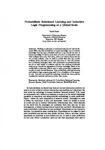
Figure 2.1: An overview of the Tether system. See Fig. 8.5 for the txt2rdf pipeline.

the average lay user. This, in a nutshell, is the practical basis for the work: dispense with all the separate data structures and hold everything in the same format. Figure 2.1 illustrates the proposed system, which takes in material from different sources and converts it into a unified graph format. Every triple has exactly the same form as every other, and each has its place within an organised schema, itself defined using triples. The details of the RDF design are covered in Sect. 3.3 and the schemas are listed in full at Appendix A. I propose a generic schema design suitable for any cultural heritage dataset, based around the “People, Places, Events and Things”, or “Who? What? Where? When?”, model commonly used in that domain. Actually accomplishing the three transformations—of database, text and various thesauri—turns out to be a major undertaking. Much of the work carried out has been exploratory research into how best to tackle it: deciding what can be automated and what should be hand-tailored, where the graph needs pruning for efficiency and how data from different sources should be mingled. For example, there are simple and obvious approaches to dealing with structured database fields, but in order to create a system with the compact schema desired these basic methods need to be altered substantially (as described in Chap. 5).


2.3

8

Natural Language Processing Tasks

The method used to translate text into graph triples is Relation Extraction (RE), a technique rapidly becoming established as a key task within NLP. My approach uses another well-established NLP technique, Named Entity Recognition (NER), as a preliminary. (See Sect. 3.1 for a review of NER work, and Sect. 3.2 for RE.) Named Entities (NEs) are the content-carrying terms in a piece of text, such as dates, the names of people or places or, in the RCAHMS dataset, the names of historic sites and the terms that classify them. The NER step consists of recognising such terms within the text and labelling each according to which category (“date”, “place”, “site type” and so on) it belongs to. Once this has been done the RE step involves searching for relationships between pairs of NEs and labelling the relationship appropriately using, for example, “has location” for a link between a historic site and the place name of where it is. A machine learning approach to the NER and RE steps is taken, using a specially annotated corpus of RCAHMS data based on a random selection of database free text fields. All of the text is in English. Before the NER step can be done the text from all sources has to be formatted as individual documents, each with a unique identifier that can be tied to a record in the relational database. Then each document is pre-processed using a sequence of standard NLP techniques: tokenising, sentence and paragraph splitting, POS (part of speech) tagging. Tokenising means splitting the text up into separate units called tokens, which roughly correspond to the words but also deal systematically with punctuation, abbreviations, apostrophes and so forth. In the POS tagging step, each token is assigned a label indicating its part of speech in the given context. The labels used are taken from the Penn Treebank2 set where, for example, “NNS” is a plural common noun and “VBD” is a verb in the past tense.3 These preliminaries are needed to get the text into a suitable format for the NE recogniser to work on. The entire sequence of NLP steps is combined as a Natural Language processing “pipeline” that takes in raw text and outputs triples, by reformatting the RE output into RDF. The pipeline is described fully in Sect. 8.4. 2 http://www.cis.upenn.edu/˜treebank/ 3 See

http://www.comp.leeds.ac.uk/amalgam/tagsets/upenn.html for a list of the POS tags with explanation of their meaning. The (much longer) definitive guide is at the main Treebank site.


2.4

9

Improving Retrieval and Presentation

My contention is that, once all the relevant information has been translated into the standardised format of an RDF graph, retrieval becomes more flexible. For one thing, it is possible to run meaningful queries across RDF with very limited schema knowledge. In a relational database, using SQL4 queries, the relationships and entity attributes have to be known in advance; in effect one can only look for what one knows is there, and web query interfaces can only allow users to fill in gaps in predetermined query commands. Using SPARQL5 over RDF, the query works by subgraph matching, and the subgraph can be as under-specified as one wishes. This means that it isn’t necessary to know what the relationship between data items is, only that one is interested in contexts in which they are related: in other words, one can construct SPARQL queries without knowing what the graph predicates are called. Another possibility, easier in a graph than in a relational database, is to create a query mechanism that can guide the user through the data by summarising across subcategories. If the query is too vague, and produces too long a list of hits, one can analyse the list by adding up frequency counts within each of the attribute groups (such as location, period, associated persons, etc.), and present the user with an intermediate summary giving some context to their request. The user can be invited to refine the original query by picking additional attributes from the summary information. This kind of approach is now becoming popular in query applications (particularly in cultural heritage), and it—or something quite like it—is usually known as “faceted search” (see, for example, Tudhope and Binding [2004]). For example, suppose the query is for “burial customs”. In CANMORE (the existing query interface on the RCAHMS website) this will produce over 2,500 hits in either alphabetic or geographical order with no subdivision between, say, 20th Century or Iron Age burial grounds. It would be helpful to provide instead an intermediate response grouping the hits by period, location and so on, and then generate a better query as a second step. I argue that strictly limiting the predicate set (i.e. the number of different graph edge labels that can be used) is a prerequisite for summarisation in practice. It reduces the number of categories or “facets” to search within, so that analysis by category at query time becomes a computationally tractable proposition. Another advantage of having a very simple schema, with a small number of predi4 Structured

Query Language—the standard way of accessing RDB data. Protocol And RDF Query Language—established in 2008 as the recommended query language for RDF. 5 Simple


10

cates, is that it can be interpreted by software agents without enormous programming effort. A generic cultural heritage RDF schema, such as is proposed here, would enable standardised web services to explore distributed datasets and assemble results from them in a way that is quite impossible at present. Many portal sites already exist in the cultural domain, but all are specifically designed for particular databases and have generally taken years to develop. The whole procedure outlined here is adaptable to related datasets in the same domain, and could potentially deliver a distributed but connected web of cultural heritage data. The matter of presentation is clearly linked to retrieval. One of the difficulties for organisations that want to make their material available to a wider audience is that it may not be in a suitable form for presenting to the target audience. A text written for professional archaeologists may be almost unintelligible to, say, a school-child studying Scottish history. Ideally one would like to be able to present information on the same topics in different ways to different types of user, and perhaps even in the reader’s native language. The subject–verb–object triple of RDF irresistably suggests the possibility of using Natural Language Generation to turn the data back into (simpler) text when it is presented to the user. The M-PIRO project [Isard et al., 2003] produced a system for doing exactly this, using a small hand-built ontology. In principle at least, that ontology could be replaced with a large RDF database, which suggests exciting possibilties for future work. When one considers the scope for integrating the graph with geospatial and multimedia data, the opportunities really seem almost unlimited.

2.5

Populating the Semantic Web

The advantages of using a graph format have been explained above. Even if they were less clear, if the present Web does turn into the Semantic Web then it is vital that historical information does not get left behind. Few would want to see educational resources limited to what has been generated in the digital era only, yet we are approaching a situation where “If it’s not on the Web, it’s not knowledge”. (See, for example, Bilal and Kirby [2002] on the strong preference for web information over traditional libraries amongst school-age children.) It is therefore important to find ways of automatically converting data—especially natural language text, which has been our preferred medium for storing knowledge for at least two millennia—into the latest formats, extracting structure from it in the process so that it can hold its own in the next generation Web.


11

The Semantic Web has actually been around for quite a long time. Its history and development are covered in Sect. 3.3, where it is noted that the first reference to it was made as long ago as 1994. The fact that adoption has been so slow—compared with the phenomenal growth of the original World Wide Web—is an indication that putting data in the necessary format is not as straightforward as one would like. Nevertheless, interest continues to grow steadily and it may be that, once critical mass is reached, expansion of the Semantic Web will be explosive. The basic idea is that information is held in as granular a form as possible, and each tiny piece of data is individually located in the giant RDF graph by its own URI.6 A query from anywhere in the world will be able to pull together very specific statements from remote data providers if it knows, or can work out, the correct URIs. This means that URIs have to be generated for each and every data item that one wants to publish on the Semantic Web. The production of suitable URIs turns out to be a very involved process, and is discussed at some length in Chap. 5. A choice has to be made between making each URI carry the full provenance of the data item (which database field it came from, perhaps which language it is in, maybe some temporal reference to when it existed etc.) or alternatively aiming for simpler, canonical references to actual things or “resources”, such as a particular person or place name. The latter approach is preferred in Tether, as explained in Sect. 5.2.2, mainly because it allows what I refer to as “serendipitous linking”, where separate references to the same thing become automatically aligned in the graph.

2.6

Sampling and Scalability

The data used for Tether is a complete snapshot of a real archive, rather than a subset, or a portion of relatively “clean” material, such as is often used in research projects. The decision to use the entire dataset was fundamental to the planning of Tether and there are a number of reasons for it. Many of the component tasks would have been faster and easier with a smaller set of tidier data (i.e. a set with more standardised record lengths, fewer non-ASCII characters, and so on) but nevertheless using the whole dataset, “warts and all”, still seems the right choice. It is an established principle in statistical NLP that one cannot have too much train6A

URI (Uniform Resource Identifier) gives either a location on the Web where a resource (such as a document, file, image, or RDF node) can be found, or just a name for it (without an address). Very commonly, URIs are Web addresses using the HTTP protocol. Each distinct resource node in an RDF graph has a separate URI. See Sect. 3.3 for a description of RDF graphs.


12

ing data. Improved results have frequently been obtained simply through having a larger sample. The components of the Tether pipeline that use machine learning methods are the NER step (see Chap. 7) and relation extraction (Chap. 8), and in these cases an annotated corpus of around 1,500 documents is used for training and testing (see Sect. 4.3), not the entire dataset—for the practical reason that it would be impossible to annotate all of the 216,000 documents that were available—but this is the exception to the rule of using the whole RCAHMS dataset wherever feasible. It was found (see Sect. 8.2.4.1) that there is considerable variation within the corpus, suggesting that, if one wanted to work with only a sample instead of the whole dataset for the main graph, it would be difficult to ensure a representative sample. Another reason for not using a subset of the data (except where forced to, as just explained) is that it makes it much more difficult to design queries and to compare their power with what can be done using existing tools against the relational database. One would have to choose a subset based on some attribute—such as all the records for a particular part of Scotland—which automatically limits the queries over the selection feature (location in this example). Furthermore, the need to choose a coherent subset is probably at odds with the desire for a representative sample. No attempt is made to prove consistency over the whole graph, which in any case would probably be beyond the power of existing reasoning tools. In fact there seems no reason to suppose that “real-world” data will be consistent: it is full of statements of opinion and of facts that are only true at a certain, often unstated, time. As is argued by Fensel and van Harmelen [2007], a lot of current research on Semantic Web reasoning uses small, consistent and static domains, and will not transfer to Web-scale. There is a need to build larger resources such as that produced here. Thus the main reason for wanting to use as much of the RCAHMS data as possible was to build a really useful,7 large RDF graph as one of the outputs of this programme of work. On the other hand sheer size was not the issue—on the contrary, strenuous efforts were made to prune the graph to a fraction of the size it could have been (see Sect. 5.2). The RCAHMS dataset provides a test-bed of manageable size that encompasses plenty of variation, with a final graph size of over 21.7 million triples. 7 Section

graph.

11.1 discusses potential future research projects made possible by the creation of the Tether


2.7

13

Research Objectives

This chapter has tried to give a flavour of the ideas that are central to this work, and the range of possibilities that flow from the simple proposition of unifying hybrid data. More options have been suggested than could be attempted by one person in less than a decade of work, so it is now time to retrench and stipulate what the necessarily limited ambitions of this thesis are.

2.7.1

Formal Goals and Evaluation

2.7.1.1

NLP tasks

Two of the main component tasks are named entity recognition and relation extraction. These were each evaluated against the gold standard provided by an annotated corpus of RCAHMS material. Neither of these tasks is absolutely central to this work so only a limited amount of time could be allocated to each. Nevertheless some new contribution is made in the NER work in dealing with nested entities, and also in the RE task which is applied to a new domain where results were not previously available. 2.7.1.2

RDB to RDF conversion

Exploring ways of translating RDB data to RDF is an active research area (often referred to as “RDB2RDF”) and a W3C Incubator Group is currently working towards producing guidance on best practice. Two contributions are made to this field: a) A checklist of recommendations for RDB to RDF translation in any domain. b) A schema design that is generic for the cultural heritage domain. 2.7.1.3

Comparison of RDB and RDF retrieval

The final graph produced was evaluated through retrieval tasks, with two sets of experiments being carried out. As explained in Sect. 3.4, SPARQL is now established as the standard RDF query language, so it was used in all the retrieval experiments. The first experiments compare queries against the original RDB data with ones over the RDF graph. The aims were: a) To assess whether queries for the same information are possible with each method (SQL over RDB tables and SPARQL over RDF).


14

b) To compare performance in terms of retrieval time. 2.7.1.4

Retrieval over text relations

The second set of experiments examine queries over the RDF graph extended through the addition of the relations derived from text. The aims were: a) To evaluate the augmentation of the graph with text relations, by finding queries that cannot be answered without the presence of the text relations. b) To assess the possibility of faceted search.

2.7.2

Informal Goals

The project has other very real but unquantifiable objectives. The main one is to explore the use of graph data on a large scale and assess whether the proposed transformation to a Semantic Web format is actually worthwhile. Is this really the “next big thing” in serious data curation work? Is the relational database on its last legs? Formal evaluation measures are helpful in such an assessment but there are issues (such as usefulness, elegance, scalability, usability, longevity, portability and other such nebulous but crucial concepts) that are difficult to measure numerically. The second area of interest is to examine how well disparate NLP and database techniques work in combination instead of independently. Most published evaluations concentrate on a single tool, but it is not obvious that separately high-performing tools will necessarily work well together, nor that they will transfer to a specialist domain like cultural heritage. The final objective is to produce a robust data structure that can form the foundation for future work. As has been explained, there are countless possibilities inherent in having a real dataset available in graph form.

2.8

A Note on Terminology

It may be useful to explain some of the terms that will recur throughout this document. The RDF data model is a directed graph of triples.8 An RDF triple consists of a subject node and an object node joined by an arc or edge (to use standard graph terminology) pointing from subject to object. The arc is known synonymously as a 8 See

Sect. 3.3 for a description.


15

“property” or a “predicate”, as one can think of the triple as expressing a given property of the subject and pointing to its value. The term “attribute” is sometimes used for the same thing. In a parallel set of terminology, it is sometimes helpful to think of the triple as subject–verb–object, where the subject and object have their normal syntactical meanings, so the triple expresses a declarative statement. In this guise, an RDF graph is a collection of “things” connected by “actions” they perform or experience. The word “ontology” crops up a great deal in discussion of the Semantic Web. For some authors it may mean a well defined hierarchy of classes with a set of rules governing their behaviour. Such an ontology can be operated on using various branches of logic, Description Logic being that most commonly used in Semantic Web reasoning. On the other hand, “ontology” sometimes means no more than a graph held in RDF, with at least some sort of class structure, but containing instance data as well as class relationships and not necessarily having any associated rules. Sometimes this kind of structure is called a “populated ontology”. To avoid confusion I have tried to stick to the broader but less ambiguous term, “graph”, whenever there is potential for doubt about what is meant. By “graph” I mean a collection of directed triples, such as may be stored in RDF. (The term “RDF” itself refers to the W3C recommendation [Klyne and Carroll, 2004] described in Sect. 3.3, and RDFS is the RDF schema language.) The “ontology” word has a little cluster of related terms around it, including “thesaurus” and “gazetteer”. I use “thesaurus” for a hierarchical arrangement of class terms with no ruleset. There may be other relationships present besides hierarchy (which is “subclass of” in RDFS, or rdfs:subClassOf), such as relatedness and preferred or nonpreferred. By “gazetteer” I mean a term list, generally with no hierarchical structure. Hierarchies, or subclass relationships, are sometimes expressed in the literature using “ISA” relations. To avoid confusion with instance relations expressing membership of a class, I avoid “ISA” and use “instanceOf” or “type” (rdf:type in fact) and “subClassOf” (rdfs:subClassOf). So, for example, stone+of+destiny–instanceOf– Artefact, and Artefact–subClassOf–Object. This example illustrates another convention—that instance names start with lower case letters, predicates use camel case, and class names are in title case.

2.9

Discussion and Summary

The central theme of this work is unifying hybrid data, keeping existing structure where available and using a graph format to include information from free text. This promises


16

better retrieval possibilities from the textual data, and also means that hybrid datasets like the RCAHMS one can become part of the Semantic Web, which in turn will allow greater interoperability with other resources. To accomplish the necessary component tasks a multi-disciplinary approach is required. Techniques are used from the relational database (RDB) field, from Information Retrieval and Information Extraction under the NLP umbrella, and from the Semantic Web world. Inevitably it is not always possible to go as deeply as one might like into a particular branch, because of the need to follow the critical path towards constructing the Tether graph. The specific research questions to be dealt with have been listed above. Chapter 11, which draws together the results achieved, also notes the opportunities for future work uncovered along the way.

Chapter 3 Related Work This thesis covers several separate but overlapping fields. Detection of named entities in RCAHMS documents is fundamental to the text-handling aspects, and dealing with nested entities is particularly important when named entity recognition (NER) is used as a step towards relation extraction, as in this programme of work. Section 3.1 looks at relevant work in the NER field. The extraction of relation triples from text has been approached in a number of quite different ways, and a brief survey is given in Sect. 3.2. The extracted relations are held as an RDF graph, which leads us on to the Semantic Web (Sect. 3.3) and graph query languages (Sect. 3.4). Section 3.5 looks at automatic ontology building. The term “ontology” is used by different people to mean different things and I have generally stuck with the broader but unambiguous term “graph”. Nevertheless, what is known as “ontology building” is relevant here, and some of the main research systems are examined. When large datasets are translated to RDF the management of the graph data is an important consideration. A lot of research has been done in recent years on storing large RDF graphs efficiently, and Sect. 3.6 gives an overview of work on triple stores.

3.1

Named Entity Recognition and Nesting

Named entity recognition is the process of finding content-bearing nouns and noun phrases within a text using rule-based or statistical approaches or a combination. It is generally considered as an Information Extraction task with two parts: finding the entity boundaries and then categorising the text strings found into types. The text strings are “entity mentions” that refer to unique individual entities. For example, “Mr. Salmond”, “The First Minister” and “Alex Salmond” are all entity mentions for the 17

Chapter 3. Related Work

18

same NE, of type “person”. Successful NER systems have been available for over a decade: see Bikel et al. [1997] for a description of “Nymble” or Borthwick et al. [1998] for “MENE” (Maximum Entropy Named Entity). These systems both used machine learning (Hidden Markov Models and a Maximum Entropy model respectively) with a set of features extracted from training data, to find entity mentions in seven categories: person, organisation, location, date, time, percentage and monetary amount. The categories to be recognised depend very much on the subject domain of the text. In general texts the traditional classes are the names of people and places and so on, as listed above, but a great deal of work has been done in bioinformatics and the life sciences where the categories are usually gene names, proteins and so on (see, for example, McDonald and Pereira [2004], Settles [2004]). Natural Language Processing (NLP) for cultural heritage is a growing field (see Sect. 4.4) with another specialist set of domain terminology for NER work. In non-specialist domains, such as newswire texts (where simple features like capitalised words work well), NER can be considered a solved problem, with the best recognisers achieving F-scores1 of 90–93% (compared with human performance of around 97%). Performance in specialist domains or with multilingual text is usually a good deal lower—typically in the region of 75–80%— though naturally it depends very much on how many entity categories are used and how well differentiated they are. Various conferences have evaluated NER systems in shared task competitions, in particular MUC2 and CoNLL3 . The CoNLL 2002 and 2003 competitions are particularly good sources of information (see, for example, Malouf [2002], Curran and Clark [2003b]). The “CandC” system [Curran and Clark, 2003a] used for NER in the construction of Tether was developed for CoNLL-2003. It is not uncommon for entity strings to contain shorter entity names within them. The following string shows three levels of nesting (each entity mention is delimited with square brackets and the NE types are shown in superscript): [[[Edinburgh]PLACE University]ORG Library]ORG The outermost entity, “Edinburgh University Library” is an organisation and so is “Edinburgh University”, whilst the innermost entity is a PLACE, “Edinburgh”. When entities are being detected as a step towards finding relations between them, as here, 1 The F-score (sometimes “F1 score” to distinguish it from variants) is the standard measure used in tagging or categorisation tasks such as NER. It is the harmonic mean of precision (P) and recall (R): 2PR/(P + R). 2 Message Understanding Conference, http://www-nlpir.nist.gov/related_projects/muc/. 3 Conference on Natural Language Learning, http://www.ifarm.nl/signll/conll/.


19

nested entities are of especial interest, as there is almost always a relationship between the levels: Edinburgh University Library is part of the University, which is located in Edinburgh. These useful relations are missed altogether if the entity recogniser cannot cope with nesting and, by contrast, are almost free gifts if it can. Interest in nested NE detection has increased in recent years, though it is still the case that most NER work deals with only one level at a time. Various methods documented in the literature are examined in Chap. 7 (Sect. 7.1) before going on to describe my experiments using a novel approach to the problem. A problem in NER is how to recognise the same entity in the multiple different surface forms in which it will be encountered. This problem is variously known as coreference resolution, deduplication, normalisation, schema matching, merge/purge, and record linking—depending on the field in which it arises. For an approach from a database viewpoint see Hernandez and Stolfo [1995]. In contrast, Ng and Cardie [2003] and Uryupina [2004] describe methods from the linguistics field.

3.2

Relation Extraction

Methods of relation extraction (RE) range from those using exclusively hand-crafted patterns and rules at one end of the spectrum, to those relying entirely on probabilistic methods at the other. Very often, a combination of approaches is employed, perhaps seeding machine learning with hand-written rules, or alternatively using supervised learning as a first step to inform manual pattern design (as in Huang et al. [2004], described below). Riloff and Lorenzen [1999] exemplify the pattern-based approach, using “signatures” such as (passive verb + ‘‘murdered’’) augmented with “slot triples” of the form (event-type, slot-type, feature), such as (murder, perpetrator, T E R R O R I S T)

and

or (murder, victim,

MILITARY

M I L I T A R Y ),

where the labels

TERRORIST

identify classes to which individual terms in the source text belong.

The only prior annotation required is in assigning a classification to each text; this is used to work out relevancy scores for the signatures detected. The approach is fairly similar to that of Schutz [Schutz, 2005, Schutz and Buitelaar, 2005] who uses a handbuilt ontology (for a football domain) as the starting point, corresponding to the “slot triples” described by Riloff and Lorenzen. The method involves several standard preprocessing steps such as POS (part of speech) tagging and NER,4 but also uses deeper 4 Refer

to Sect. 2.3 for a description of basic NLP tasks like POS tagging.


20

analysis to determine grammatical functions like subject and object. Relevance within domain is assessed using a χ2 test (see, for example, Manning and Schütze, 2002, p169). Another approach [Huang et al., 2004] extracts the patterns automatically— by aligning word sequences between sentences and looking for similar portions—and then filters the candidate patterns using hand-written rules. The drawback with most machine learning approaches is the need for annotated data, whilst the alternative of hand-coding detailed and specific rules may be as timeconsuming as doing annotation. Unsupervised methods which can learn from unannotated raw text are therefore of great interest, and Yangarber and Grishman [2001] provide an example for relation extraction over large bodies of text. They start with a small set of seed documents known to be relevant to a topic and try to deduce patterns from them by looking for pairs of co-occurring entities and examining the phrases containing them (for example, company and location names in strings such as “company X is located in Y”, “company X has headquarters at Y” and so forth). So far this has a certain resemblance to the work described above, but Yangarber and Grishman add an active learning element, by asking an interactive user for similarity judgments in the least certain cases, instead of relying on preclassification and statistical tests. In the ODIE system (On-demand Information Extraction) [Sekine, 2006], the aim is to minimise the effort of transferring to a new domain by first using TF-IDF5 retrieval to obtain a small set of documents (from a news domain) to work with, and then automatically generating patterns for relation extraction from them using a dependency analyser. Only the patterns that contain previously identified named entities are used, after the NEs are found by a specially developed rule-based tagger—which presumably entails some degree of domain tailoring. Another issue in tailoring to new domains is determining the relation types, and the goal of doing this automatically has been addressed by various authors; see for example, Hachey [2006], who proposes a method for clustering pairs of co-occurring entities so that each cluster can be allocated a relation label. In the development of Tether some experiments were done to assess the possibility of automatic derivation of relation type labels, by finding the highest frequency verb phrase types and then clustering them using the “Similarity” measure developed by Pedersen et al. [2004] over WordNet [Miller et al., 1990], following the lines suggested by Budanitsky and Hirst [2006]. Results were inconclusive and a pragmatic decision 5 “Term

Frequency – Inverse Document Frequency”: an indexing method that assigns high weight to terms that, whilst being comparatively rare in the corpus as a whole, occur frequently in a particular document and are therefore good indicators of the document topic.


21

was made to determine the relation types by hand, on the basis that it is a task that only has to be done once for each domain and needs to be reliable as a foundation for the rest of the RE work. While most methods of relation extraction start with some linguistic analysis steps, some (such as Schutz 2005, mentioned earlier, and Riedel and Klein 2005) do full parsing, to extract relations directly from the sentence structure. Riedel and Klein go further, and experiment with inference rules over the resulting relations. For these approaches a lexicalised grammar, such as CCG or link grammars, is needed. There are various tools which will convert parses in such grammars into discourse structures with semantic labelling. I carried out some experiments with Cass (by Steve Abney), CDE6 [Bos et al., 2004, Bos, 2005] and a Link Grammar parser [Sleator and Temperley, 1993] to assess full parsing as a route towards RE for Tether, using a small, randomly chosen sample of sentences from the RCAHMS corpus. This line was not pursued further however, partly because too little of the RCAHMS text is in grammatical English sentences for the parsers to succeed, and partly because of speed considerations where the ultimate aim was to deal with hundreds of thousands of documents. There are a number of toolsets and general purpose utilities for Information Extraction (IE) and some of these now include relation extraction tools. An example is the CAFETIERE suite developed at Manchester University [Black et al., 2005], which is based on the GATE (General Architecture for Text Engineering7 ) software and uses mainly hand-crafted rules to extract two place relations between pairs of entities. GATE itself arose out of the earlier TIPSTER architecture and, as described in Cowie and Wilks [2000], forms the framework underlying other IE tools like VIE (Vanilla Extraction System) and LaSIE. In general, interest in the relation extraction problem has grown considerably over the last few years. The NIST-sponsored ACE (Automatic Content Extraction) programme8 has been running since 2000, with research goals of detecting and characterising entities, relations, and events. Each year since 2001 there has been an increasingly ambitious series of competitive tasks, including relation detection and recognition (RDR)—though in 2008 the complexity of the tasks has been scaled back, to include only one entity and one relation task, EDR (entity detection and recognition) 6 CDE

stands for “CCG and DRT Environment”. It is a package that translates CCG (Combinatory Categorial Grammar) output to Discourse Representation Structures (DRS), as used in Discourse Representation Theory. 7 http://gate.ac.uk/ 8 http://www.nist.gov/speech/tests/ace/, http://www.ldc.upenn.edu/Projects/ACE/


22

and RDR. Evaluation results for the RDR task are available for 2005 and 2007. Instead of precision and recall measures ACE uses its own scoring method based on matching outputs against a reference set in which each relation (in the case of the RDR task) has a collection of attributes. The system under evaluation is scored according to how well it reproduces the attributes and their values. The maximum score is 100, for a perfect match, but negative scores are possible if spurious attributes are produced. In 2005 the published scores for the RDR task on English text were in the range 20.1 to 25.2. In 2007 the best RDR score was 21.6. The ACE tasks are complex and include many more characteristics of text relations than are needed for the purposes of Tether, where the aim is to find pairs of related entities and label the relationship between them. This produces an RDF triple, where each entity corresponds to a resource node and the relationship label becomes the predicate for the arc joining the two nodes. Broadly similar kinds of problems are dealt with in otherwise unrelated fields. Statistical Relational Learning [see Neville et al., 2003, Popescul and Ungar, 2003, Bunescu and Mooney, 2004] is concerned with machine learning to extract latent information about correlations of data items, typically in relational databases (RDBs) or other organised sets or matrices. (This “SRL” has no connection with the other SRL, Semantic Role Labelling, which is another possible approach to the RE task, but using linguistic dependency analysis not statistical correlation. The only similarity is that both detect connections between separate entities.) Probabilistic Relational Models [Getoor et al., 2001] over RDB data have some similarities, and in turn the Probabilistic Entity Relationship model [Heckerman et al., 2004] is a generalisation of PRMs. All of these favour conditional models, and Bayesian nets in particular. For a discussion of mining from databases with the specific aim of populating ontologies, see Meersman [2001], who also stresses the importance of database-like features for maintaining ontologies, such as ease of updating. Quite simple techniques for detecting correlations have been shown to produce useful results in data mining, such as the a priori algorithm (see Hand et al. 2001, pp. 157–160 or Han and Kamber 2000, pp. 230–239), which learns association rules from data by finding sets of entity mentions that occur together often. Where the set has only two members one effectively has a binary relation. I experimented with the a priori algorithm for Tether as it copes well with large volumes of data. One problem is that many of the correlations are not informative (“RCAHMS” with “information”, “Ordnance Survey” with “6-inch [map]” and suchlike), and another is that there is no


23

obvious way of preserving the NE category labels that are needed for disambiguating place names from personal names and so forth. Also, an extra step would be needed to allocate a label to the relationship type. For this work it was not practical to test and compare all the different approaches to relation extraction that are theoretically possible. A certain amount of preparatory exploration was done, as has been explained, before settling on the “maxent” tagger [Zhang and Yao, 2003], a general purpose maximum entropy learner, used with an annotated corpus of training material. This was chosen because it was found to be very fast, and because it was known to have been used successfully in other RE work, such as that of Haddow and Matthews [2007].

3.3

Semantic Web

What seems to be the first published mention of “the need for Semantics in the Web” occurred in a plenary address by Tim Berners-Lee at the first WWW conference at CERN in Geneva, in May 1994. (This was also the gathering at which the formation of the W3C was announced.) The presentation does not appear in the conference proceedings [Enslow and Cailliau, 1994], but there is a note of it at http://www.w3. org/Talks/WWW94Tim/Overview.html.9 The gist of the proposal was: “Adding semantics to the web involves two things: allowing documents which have information in machine-readable forms, and allowing links to be created with relationship values.” That succinct vision has not changed, but the mechanics of how to make it happen took some time. RDF became a W3C Recommendation in February 1999 (see Klyne and Carroll [2004] for the current standard), though for some time it was unclear whether or not it would become the framework on which the Semantic Web rests. Both Decker et al. [2000] and Berners-Lee et al. [2001] go into some detail on the relevant merits of XML or RDF as the preferred language for the Semantic Web. It is now clear that RDF has won, though it is often serialised in XML, as well as other formats such as N3,10 NTriples11 and Turtle,12 which are a good deal easier for human reading. The OWL Web Ontology Language13 can be used within the RDF framework 9 That

web page states it was given in September 1994, but possibly Sir Tim is misremembering the dates of WWW1 (25th–27th May 1994, Geneva). The conferences were twice-yearly until 1996. 10 http://www.w3.org/DesignIssues/Notation3 11 http://www.w3.org/2001/sw/RDFCore/ntriples/ 12 http://www.dajobe.org/2004/01/turtle/ 13 http://www.w3.org/TR/owl-ref/


24

and has more expressive power. RDFS, the RDF Schema language,14 is less powerful than OWL but allows schema relations like class hierarchies and domains and ranges for predicates to be expressed in RDF. Since RDFS does not include negation it cannot be used for inference in the way that OWL can. A comparison of the relative merits of XML, RDF/RDFS, the earlier DAML+OIL, and OWL is given in Arroyo et al. [2004]. (For a general introduction to Semantic Web languages and applications using them see either Antoniou and van Harmelan [2008] or Passin [2004].) The original vision, quoted above, talks only of machine-readable content and of links to “relationship values” (an interesting point to which I will return in a moment). Very soon this was expanded into a call for structured vocabularies and inference rules. The classic early description was in a Scientific American article [Berners-Lee et al., 2001]. This paints a picture of autonomous software agents making logical inferences using supplied rules, which allow them to provide “proofs” of the conclusions they present to their human masters. The practical goals are scenarios such as one’s telephone being able to turn down the volume of all local devices so it can be more easily heard, or a software agent looking up travel options and costs, and making bookings on one’s behalf. Following this lead, Meersman [2002] sees the Semantic Web as the solution to the “chaos” of the Internet, and proposes an agenda of work on ontology building and unifying, and also looking at issues of licensing and intellectual property. A more recent article, Feigenbaum et al. [2007], updates the 2001 paper by describing case studies of systems such as health care and drug indexing that now use Semantic Web technology. That article, also in Scientific American, is determinedly optimistic, in some contrast to the tone of Shadbolt et al. [2006], which notes that takeup of the Semantic Web vision has been disappointingly slow. This is certainly true if one compares it with the explosive growth of the original Web which, starting in late 1989 in an essentially academic environment, became within about five years a necessity for almost every commercial company in the developed world. Shadbolt et al. describe RDF, certainly as presented in XML, as “clumsy syntactically”, and speculate that this hinders its adoption; and it is hard to disagree with them. They also note the emergence of “folksonomies”15 but argue that what is really needed is an authoritative collection of standardised and maintained ontologies. By “ontology” they appear to 14 http://www.w3.org/TR/rdf-schema/ 15 Folksonomies are loose graph structures built “bottom up” by individual, usually unskilled, contrib-

utors who attach tags (short descriptive text strings) to instances of web resources such as photographs, favourite links and so on. If “critical mass” is reached, with a sufficient volume of tags, the theory is that reliable cataloguing results, essentially through preferring tags with higher frequency counts.


25

mean a hierarchical arrangement of terms (called a “thesaurus” in this thesis), not involving rules and inference; though they also call for the separate development of rules and note the creation of the RIF (Rule Interchange Format) Working Group.16 Berners-Lee is sometimes quoted as saying he wishes he had christened this new evolution the Data Web, because that describes it better: the idea is to make it as easy to link data as HTML makes it to link documents. He has also used the term “Giant Global Graph” or “GGG”,17 which is an accurate description as the aim is a distributed graph database, so perhaps we will soon be talking of “the Graph” as we now do about “the Web”. I noted above that his earliest statement of the goal talked of linking on relationship values. It is important to note that in RDF only certain types of “value” are allowed to form links, as explained below. Assuming, as is de facto the case, that Semantic Web data is held as RDF, then it is in the form of a directed graph, with nodes connected by arcs. The arcs or edge labels are known interchangeably as “properties”, “predicates” or “attributes”. Thus the data can be stored as a set of subjectNode–propertyArc–objectNode triples, often called SPO triples, and represented graphically as: subject

object predicate

The beauty of the original vision is that subgraphs will become automatically connected to one another if they (a) are exposed on the Web, and (b) share at least one common node. Figure 3.1 illustrates this principle—the node labelled “X” is identical in each subgraph so the two are automatically connected by it and, through it, nodes “Y” and “Z” are seen to be related. RDF makes a distinction between “resources”, which are full members of the Semantic Web with URIs that uniquely identify them, and literal values that are just quoted strings or typed integers or whatever. Graphically a literal is usually represented as a rectangular node instead of an ellipse: :Siteid#site1

:name

"Dirleton Castle"

This example is from the RCAHMS data, expressing the statement that the name of site1 (a resource with a URI) is “Dirleton Castle”. Only resources can be the subject of triples in RDF. This means that the graph stops when it reaches a literal, so the linking on “values” only happens if the value is turned 16 http://www.w3.org/2005/rules 17 Blog

posting in November 2007 by Berners-Lee, http://dig.csail.mit.edu/breadcrumbs/ node/215.


26

X X

Y

X

Z

Z

Y

Figure 3.1: Merger of two RDF graphs that share a common node. Node X is in both graphs, so they are automatically joined and Y and Z are linked.

into a resource with a URI. There are various ways round this, including the use of “bnodes”, which are anonymous resources intended only for this purpose. They are able to be the subject of statements without having their own URI, and their physical identification is a matter for the particular software implementation used locally. For various reasons the Tether design eschews bnodes—this knotty issue is discussed in some detail in Sect.5.2. Suffice it to say here that the cleanness of the original Semantic Web idea is somewhat compromised by the fact that one cannot, in fact, make links on what most people would consider “values”, i.e. strings. The simplicity of information retrieval by typing a string into a search engine cannot be directly reproduced in the Semantic Web, where literal strings are never the subject of statements. There seems a danger, indeed, that Semantic Web tools may be reduced to using regular expression string matching within URI names in order to cross the divide between a human’s idea of semantic meaning and a machine’s. It is interesting to note that the RDF specification permits a property arc to be a subject node as well. It is just another “resource”, which can be the subject of an as-


27

sertion. This is necessary, for example, in order to specify the domain and range of the attribute as RDF statements, e.g. picasso–paints–”Guernica”, where paints is a predicate or edge, is complemented by two schema relations defining the predicate: paints–domain–painter and paints–range–painting (where paints is a node). Clearly these two statements can themselves be expressed as RDF triples. It has been pointed out by Hayes and Gutierrez [2004]—whence these examples are taken—that RDF structures may therefore not be true graphs, because the definition of a graph requires the sets of edges and nodes to be disjoint. This means that standard graph algorithms may not be applicable in the general case. Hayes and Gutierrez show how an RDF graph can be transformed into a bipartite graph which can be always be processed with the standard algorithms.

3.4

Graph Query Languages

There is no shortage of query languages for RDF. To name some of the ones that have been developed over the past few years: RQL,18 RDQL,19 RDFQL,20 SquishQL,21 SeRQL,22 N3QL,23 iTQL,24 Triple,25 Versa,26 RxPath27 . . . and probably others. However, SPARQL28 has now been established as the standard. It became a W3C recommendation in January 2008 after a rather uneven passage over nearly four years, during which it briefly went downwards in the W3C status pyramid before finally reaching the top. See McCarthy [2005] for a useful introduction to SPARQL basics. Like most of the earlier contenders, SPARQL is based on the SQL paradigm, making its syntax easy for database practitioners to adapt to. Also like the other languages, it so far makes little use of graph querying techniques that one might naturally assume would be available but is restricted to simple subgraph matching, or “path matching”, to use the terminology of its other ancestor, XQuery, and similar XML query languages based on XPath. 18 [Karvounarakis

et al., 2002]

19 http://www.w3.org/Submission/2004/SUBM-RDQL-20040109/ 20 http://www.intellidimension.com/ 21 [Miller

et al., 2002]

22 http://www.openrdf.org/doc/sesame/users/ch06.html 23 http://www.w3.org/DesignIssues/N3QL.html 24 http://kowari.org/oldsite/1246.htm 25 [Decker

et al., 2005]

26 http://copia.ogbuji.net/files/Versa.html 27 [Souzis,

2004]

28 http://www.w3.org/TR/rdf-sparql-query/


28

The perceived gaps in SPARQL and other RDF query languages are explored in detail by Angles et al. [2004], Angles and Gutierrez [2005] and by Stuckenschmidt [2005]. Their contention is that a graph query language should let the user find paths between pairs of nodes, find all nodes within a certain distance of the current one (kneighbourhood queries), and do aggregation queries such as finding the degree of a node (i.e. the number of arcs leading from it), or the diameter of a subgraph. They refer to earlier graph database languages such as GraphLog [Consens and Mendelzon, 1990], and to various known graph searching algorithms. See Shasha et al. [2002] for a survey of the latter. Anyanwu and Sheth [2003] cover similar ground on the difficulties of discovering how RDF resources are related (i.e. the paths between them and the labels of these paths), and propose extending the current languages with their ρ-query operator29 to provide this functionality. It is not clear as yet whether SPARQL will be extended to provide graph functions, and there is room for further work to determine how necessary they are. It was beyond the scope of this thesis to answer that question but graphs like the one created here may be useful as test-beds for such research. The current version of SPARQL is a query-only language. The SQL relational database query language includes both DML and DDL commands. DML is Data Manipulation Language, including “insert”, “update” and “delete”, for changing the content held in the database. DDL stands for Data Definition Language, where the most important command is “alter”, used for making changes to the schema such as adding tables to the database, adding extra columns to existing tables and so on. There are no equivalents in SPARQL as yet for altering either individual content nodes or the schema of the graph. They will undoubtedly be needed in the future so either SPARQL will be extended or new ancillary languages will appear, to allow Semantic Web content to be maintained.

3.5

Automatic Ontology Building

For the work proposed here, extracting triple relations from text as described in Sect.3.2, is just a means towards the end of organising them, along with data from other sources, into a graph database that can be queried. This process is sometimes called “automatic ontology building”. The word “ontology” is used in the literature for quite a range of constructions. 29 The

authors use the term “ρ path” to signify an instance of a path between two nodes.


29

As part of Knowledge Management and formal logic, and in the usage closest to the philosophical roots of the term, an ontology is a tightly controlled set of relationships between entity types and a collection of rules governing their behaviour. Such ontologies are designed for organising high level knowledge and their practical application is often as business management tools [Macintosh et al., 1998, Preece et al., 2001], where they will support modelling and reasoning tasks in the related Knowledge Engineering field. This kind of ontology is generally built by hand by an experienced analyst. For a clear overview of the typical procedure see Uschold and King [1995], Uschold [1996]. In the last few years, “ontology” has come to include much less formal and wellorganised structures, where the ruleset is very much an optional extra and the relationships may be derived, “bottom up”, from links between individual instances. Thus the structure contains a collection of instance or “content” data, rather than simply being a framework of relationships between classes or types. These structures are sometimes called Knowledge Bases or “populated ontologies”. The two contrasting attitudes just described are characterised, in Brewster et al. [2004], as “Newtonian” or “Platonic” (for the formal abstract structures codifying knowledge) as opposed to “Leibnizian” or “Aristotelian” for the messy, task-dependent versions which typically don’t attempt to make universal rules about classifications, and consequently may have to tolerate inconsistencies. One of the contributors, Steve Fuller, cites a test question: “What goes with a cow: a chicken or a bed of grass?”. He argues that those with a Newtonian attitude choose the chicken (because they think in terms of hierarchies of types, and cow and chicken are examples of mammals), whereas Liebnizians will pick the grass because they look for composite pictures where constituent parts are described by their attributes or situation. A Liebnizian structure will tend not to have a well-ordered class hierarchy and will be less easy for reasoners to deal with. The Tether design aspires to take the best of both of these approaches, by fitting instances into a pre-determined class structure (see Sect. 5.3) but using a small set of fairly loosely defined predicates that permit connections between nodes widely separated in the class hierarchy. (The most obvious example is seeAlso, that can connect almost any two nodes, but is unlikely to be useful for inference.) Consistency checking and reasoning are orthogonal to the project’s aims.30 Another contributor to the same article notes that fewer than 10% of practical applications actually make use of the logical inference available in “Newtonian” ontologies anyway. It is difficult to 30 There

is no guarantee that the source data is self-consistent anyway, as it often expresses statements true only in a particular time-frame that may not be explicitly stated (and would be beyond the scope of my system to capture if it were). Users of the data are expected to exercise their own judgment.


30

assemble evidence one way or the other, but I would imagine that is still the case today. Chandrasekaran et al. [1999], who are very much at the “Newtonian” end of the spectrum themselves, describe various ontology management tools and languages such as KIF (Knowledge Interchange Format), Ontolingua and CommonKADS. The authors also look at practical systems like CYC [Lenat, 1995] and WordNet [Miller et al., 1990]. The latter is much more thesaurus than ontology, covering senses of English words. CYC is an attempt to encode “common sense knowledge”, containing (at the time of the article cited) around a million “assertions” and having taken about a personcentury of effort to build. As one might expect with a real-world system of this size, it doesn’t aspire to formal logic proofs but aims (ultimately!) towards allowing deduction by weighing competing assertions in an argument. In smaller structures where formal reasoning is a practical option, Description Logic is the prevailing framework [see Baader et al., 2003]. There is an interesting overlap between machine learning and formal rule-based logic in Inductive Logic Programming (ILP) (Mitchell 1997, Chap. 10; NienhuysCheng and de Wolf 1997). The goal of ILP is to learn rules from a large number of examples, where the rules may be simple atomic ones expressing propositions or first order rules embodying predicate statements. As part of the extraction of relations from text one could attempt to infer class or schema relations based on a collection of instances, using ILP techniques. This is beyond the scope of the present work but might be worth further exploration in the future. Automatic ontology building has been a hot research topic in recent years. The Artequakt system [Alani et al., 2003] is a particularly relevant example. It operates in the heritage domain, containing information about artists and fine-art artefacts. Starting with a hand-built ontology including a set of “biography template” rules, the authors extract subject–object–relation triples from relevant web pages, and populate the ontology with these. They use what they call “narrative generation” to produce output in response to a fixed range of simple queries; for example, a query for “Rembrandt” will produce a generated biography. This is not quite full-scale NLG (natural language generation), as the text snippets are from the original input web pages and are stored and indexed in the ontology. Another system, M-PIRO [Androutsopoulos et al., 2001, Isard et al., 2003], carries text generation a step further, constructing natural language output directly from data in a hand-built knowledge base. This could be adapted as a potentially exciting use of statements stored in a graph, which it would be very interesting to explore further.


31

There are many other descriptions of ontology building work. In some cases the process is not fully automatic, but is seeded with a hand-constructed core ontology as just described. Vargas-Vera and Celjuska [2004] provide such an example, working in a news stories domain with a small ontology containing about 40 classes, and a set of templates with slots for attributes of certain events (such as visiting a person or a place). The Ontolearn system [Navigli et al., 2003] uses WordNet as the basis to build on, or allows the user to substitute a specialist domain ontology. The method involves deducing the sense of a term within the domain to place it in its “semantic context” in the ontology, the latter being gradually updated and pruned to reflect the topic domain being worked with. It is described in more detail in Sect. 3.5.1 below. Two fully automatic methods, [Blaschke and Valencia, 2002] and [LOGS, 2004], provide an interesting contrast. The first uses a clustering algorithm to build a geneproduct ontology from the leaves upwards. At each stage the two most similar nodes are found and merged, to move up a level in the tree. The final result is a set of binary trees. The LOGS (Lightweight universal Ontology Generation and exploitation architectureS) system works exactly the other way round, identifying the root node first and working downwards from there. Supervised learning is used, over a set of documents (in a particular format) marked with a hierarchy of concepts. Concept identification is by a relevancy signature algorithm based on that of Riloff and Lorenzen [1999] (mentioned in Section 3.2 above), adapted to use statistical association rather than particular syntax elements. Another automatic system is described in Mena et al. [2000], though the domain (software packages) is restricted and only a very small set of input data is used. The purpose is not so much to demonstrate practical ontology construction as to highlight the use of software agents to convert the (highly structured) web pages into ontology graphs. Finally, it is interesting to compare recent work with a much earlier paper: Doyle [1962]. This work is in the IR (Information Retrieval) field, and Doyle explains how statistical associations between pairs of terms in large text corpora can be used to build graphs which he calls “association maps” or “semantic road maps”. He notes that classification is always context-specific, and that an advantage of graph representation is that multiple classifications can be shown in parallel: the same two nodes may be close under one categorisation but distant (either with many intervening nodes or with a “weak” link) under another. Doyle envisaged a query interface where a graph of relationships between search terms would be presented to the user, who could pick


32

terms for query expansion. Unfortunately, he was a long way ahead of his time, as the typical computer interface at the time was a character Teletype machine with a roll of paper.

3.5.1

Experimental Applications

There are many practical experimental applications based around ontology building and this section give a little more detail on one or two that seem most relevant. Many of the published descriptions concentrate on how the ontologies were constructed, but some go further and discuss evaluations of usage, a particularly interesting example being the Ontolearn system mentioned above. Its purpose is to tailor a general purpose seed ontology (such as WordNet) by expanding and pruning it, so that the result reflects domain-specific knowledge. A detailed description of the architecture is provided by Navigli and Velardi [2004]. In an earlier paper [Navigli and Velardi, 2003] the authors explain how they deal with queries over the graph structure they have built. They take a graph-centric view (talking in terms of subgraphs and paths between nodes), in contrast to Semantic Web work which tends to be database-centric (using terminology tied to class membership and relations between instances). The procedure is to take each query term and expand each sense of it into a “semantic network” (a subgraph of all relations linking to the term, up to a certain distance from this root), then these subgraphs are intersected by finding common nodes that can be reached from each subgraph root by directed paths. Terms on the intersection paths may be expanded to semantic networks themselves. It is important to note that this type of graph function is not possible in the standard RDF query languages like SPARQL, as discussed in Sect. 3.4. Experimental results were generally very good, except when the intersection path passed through terms representing high level concepts, which caused the results to branch away from specifics too much. There was also a problem with named entities: Ontolearn does not include NER, and the application attempted to expand NE terms (which it did not identify as “special”) to semantic networks, with poor results. The authors recognise that such expansion should be limited to concept terms, the best candidates being terms in the same semantic domain and same level of generality as query terms. Expanding with gloss words (derived from WordNet concept definitions) worked well. There are quite a number of other ontology application projects. Although mainly concerned with building an ontology of geographical entities, Alani [2001] is of inter-


33

est because the source data is the same as mine, from RCAHMS. Volz et al. [2003] describe the KAON ontology project which is implemented on the Sesame triple engine. The OBIIE system (Ontology-based Interactive Information Extraction) is a query application allowing sophisticated queries like “keyword1 plus keyword2 in a verb group”, over scientific abstracts from EMBASE and MEDLINE [Milward et al., 2004]. The DOPE project (Drug Ontology Project for Elsevier) also works with EMBASE source data [Stuckenschmidt et al., 2004]. The Gene Ontology project deals with gene and protein terms, and the term hierarchies are described in detail in Ashburner et al. [2000]. Milward and Thomas [2000] describe an interesting query application that treats seriously the difference between index time and search time functionality. The source data is heavily pre-processed at index time, occupying up to 60 times its original space, but the search time is estimated to be one tenth what would be needed if the processing (on a subset of the data) were done at run time. (Compare the remarks about denormalisation in Jena 2 in Sect. 3.6.1—disk is cheap, and unless one aims to process the entire database in memory, pre-clustering and so forth seems sensible, for a query-only application.) However, in this particular application the volume of the pre-processed data means that loading even sections of it for run time searching is slow, so fast IR tools are used as a filter first. The method is a hybrid between traditional IR and IE, and offers the user a choice of results formats: either a list of document links (as in an IR system) or a tabulated set of fields (the IE style). A similar approach trading very extensive pre-processing against fast retrieval is used by Jijkoun et al. [2003], although the user interface is different as theirs is a Question Answering (QA) system. In QA the aim is to extract from a data source brief answers to factoid questions. Jijkoun et al. extract a table of “facts” from the document collection, using finite state methods, and analyse each query to see if any of the extracted facts can be matched as an answer to it. The building of a collection of facts is analogous to ontology construction. There is a huge body of work on Question Answering—which overlaps with ontology querying in that both are concerned with information retrieval to answer queries—but I won’t attempt a bibliography of QA here. For helpful overview material on this field, see Hirschman and Gaizauskas [2001], Burger et al. [2001], Voorhees [2003]. Similarly, the IR and IE fields will not be covered here, save to mention some useful general texts that were used for reference: Baeza-Yates and Ribeiro-Neto [1999], Witten et al. [1999], Sparck Jones and Willet [1997], Strzalkowski [1999], Cowie and Wilks [2000].


34

The CultureSampo [Hyvönen et al., 2007a] and FinnOnto [Hyvönen et al., 2007b, 2008] projects hardly deserve to be described as “experimental”, as they have moved outside the Helsinki University of Technology to embrace real data from an impressive range of cultural and other archives in Finland. For FinnOnto, the team from SeCo (Semantic Computing Research Group, see http://www.seco.tkk.fi/) co-ordinated the construction of an “upper ontology” or concept hierarchy in order to provide a framework for Finnish data on the Semantic Web, in a diverse range of subject areas: culture, health, government, education, and commerce. The related CultureSampo project is cross-domain with heterogeneous content. It uses event-based modelling, which makes it easy to represent facts as relations between events and their agents or patients. (Figure 3.3 shows an example of RDF modelling using reified events.) This also means the metadata is more interoperable and more likely to form a working part of the wider Semantic Web. Search results are presented using faceted search (see, for example, Tudhope and Binding [2004], Hearst [2006]) plus what they dub “relational search” (e.g. “How is Picasso related to Paris?”). The presentation interface also uses mashups with Google maps and time-lines. Despite its breadth of scale, FinnOnto lies towards the “Newtonian” end of the spectrum (see discussion on page 29), and may establish itself as a counter-example to the implied scepticism about reasoning being feasible over big “real-world” datasets—it is too early to tell. The MultimediaN (“Multimedia Netherlands”) E-Culture project [Schreiber et al., 2006] is another recent and impressive project that uses Semantic Web technologies over virtual cultural heritage collections. Like CultureSampo, it includes a search function for discovering semantic relations between URIs, to answer questions like “How are Van Gogh and Gaugin related?”. Integrating standard vocabularies (such as the Getty ones—see Sect. 4.2.1) is a central goal of the MultimediaN project, and Tordai et al. [2007] describe how this is done, based around the RDF SKOS schema and using the Mapping Vocabulary31 to build alignments between separate but related thesauri.

3.6

Managing Triples

Small RDF graphs are often implemented as flat files (serialised in XML or some other representation) and loaded into memory for processing, but this is not currently 31 The SKOS Mapping Vocabulary is now deprecated but the important relations from it have been taken into the core SKOS standard, see http://www.w3.org/2004/02/skos/vocabs.


35

practical for a large archive (of more than a million or so triples). The graph must be held in persistent storage in a specially designed store that permits small sets of triples to be extracted by queries without attempting to build the entire graph in memory. There are now quite a number of rival triple stores and a good deal of work has been done on how best to structure them. As well as reviewing the relevant literature, this section explains the criteria by which the Jena32 and AllegroGraph33 systems were chosen for Tether. Although RDF has become the standard it is not the only possible implementation method, and a rival known as the Associative Model is also examined, in Sect. 3.6.3.

3.6.1

Persistent Triple Stores

An effective triple store can be produced with a structure as simple as a single threecolumn held in a relational database: each SPO triple appears as a row in the table. (Since a table, or relation, is a set—with no duplicate entries34 —this is a very convenient implementation for a set of triples making up a directed graph in RDF.) In practice most triple stores add a “graph ID” as a fourth member of each relation (i.e. a fourth column in the table definition), to tie each statement to its parent graph. Thus the SPO triple becomes a quad: SPOG, where “G” is the graph identifier. This facilitates segmenting and joining of multiple graph databases. The SPARQL language has provision for specifying whether the default graph or a specific named graph is to be queried, using a mechanism analogous to the namespace principle in XML. See Carroll et al. [2005] for a description of named graphs in RDF. The syntax allows one to assign a URI to identify an entire graph, which can then be used as the subject node in RDF statements—this allows metadata pertaining to the dataset as a whole (such as provenance information) to be stored alongside the actual content data. Another pragmatic variant on the single table model is the use of ancillary tables holding indexes to the resource URIs and literal strings so that these often cumbersome values do not have to be repeated in the main table. Instead they are coded and pointers are used to track them. There are a number of RDF data storage systems now available: Kowari,35 Sesame,36 32 http://jena.sourceforge.net/ 33 http://agraph.franz.com/allegrograph/ 34 Not

every RDB implementation enforces the rule that a relation should not contain duplicates but it is easy to ensure it using SQL functions. 35 http://www.kowari.org/ 36 http://www.openrdf.org/


36

3store,37 RDFStore,38 Jena (which includes Joseki,39 as part of its framework), Mulgara40 (which came out of the earlier Kowari project), Dave Beckett’s Redland RDF Libraries41 and AllegroGraph are amongst the most popular. Several of these use a relational database as a back-end store, particularly for RDF datasets that are too large to hold and process in memory. The 3store system uses MySQL for preference and structures the RDF data in a single table with a few auxilliaries, as outlined above, see [Harris, 2005]. HP’s Jena system employs a similar four-column table layout [HP, 2004], though in Version 2 the structure was revised to include less normalisation with pointers, as the de-referencing step was found actually to spoil performance. Oracle Corporation have implemented a commercial RDF store as part of their Version 10g database [Alexander et al., 2005, Oracle, 2005]. All of these implementations are relatively new as yet, and there are few examples of really large RDF databases in day-to-day use (at least in what one might call “business critical” positions). The system initially chosen for Tether was HP’s Jena, which was the best available at the time, in terms of design, transparency of implementation (one can access the store directly through SQL in the RDB back-end), robustness, good documentation and usable API (written in Java). As a company, HP has been one of the leaders in Semantic Web research, and Jena remains one of the most solid platforms available. Its only failing is that it is slow (at least in comparison with AllegroGraph): both loading and retrieval performance are disappointing when the graph contains many millions of triples (see Table 5.3 for the bulk loading statistics). As mentioned earlier, the Tether graph contains over 20 million triples. Later on in the development work AllegroGraph, from Franz Inc., was used alongside Jena (which by that time had changed so significantly that a re-install was needed anyway), so that comparisons could be made between two of the best available systems. AllegroGraph was developed recently and takes advantage of earlier work in the field. It was built using Lisp but also has a Java interface. (Although AllegroGraph is a commercial product, there are free Lisp and Java editions that are fully functional but limited to 50 million triples. Franz Inc. very kindly made the commercial version available for this work, though in fact Tether fits in the free version.) The AllegroGraph design does not hold literal and resource strings directly but uses 37 http://www.aktors.org/technologies/3store/,

and see [Harris and Gibbins, 2003]

38 http://rdfstore.sourceforge.net/ 39 http://www.joseki.org/ 40 http://www.mulgara.org/ 41 http://librdf.org/. The Redland suite includes utility libraries for numerous RDF manipulation tasks, as well as triple storage and querying.


37

hashed codes—called UPIs or Unique Part Identifiers (not, of course, to be confused with URIs!)—as pointers. More controversially they also add a unique Id to each triple (for internal query efficiency), and suggest it could be used to allow one triple to refer to another without RDF reification.42 This is in fact precisely the Associative Model of Data described in Sect. 3.6.3 below. AllegroGraph also has the usual graph Id, so each “triple” is actually a quint: SPOGI, where an “I” statement identifier is added to the usual SPOG set. As an aside, it’s interesting to consider whether such a cavalier attitude to the RDF standard on the part of a commercial developer is a disaster, or a welcome sign that triple-stores are coming out of the ivory towers. Franz have clearly got to grips with how a real database should work—which may be why their system appears to be at least an order of magnitude more efficient than most others, in handling multi-million row triple stores. Semantic Web tools will surely need to be robust and fault tolerant to succeed—just as HTML was—and that means taking variants like this in their stride. The loading and indexing performance of AllegroGraph is remarkably good, as shown in Table 5.3 (on page 103). One drawback is that the storage engine is a proprietary one instead of a standard RDB, so one cannot easily get inside it as one can with Jena (which I run over MySQL).

3.6.2

Retrieval from RDB Triple Stores

If an RDF graph is represented in a relational database then a query that needs to move around the graph, from node to node along paths, will require multiple self-joins of the main triples table. A relational join is made by matching an attribute of one table or relation with an attribute of another; the matching function is typically, but not necessarily, equality. It is a self-join in the case where the join is made between a table and a copy of itself, which is necessary when one wants to link data in one part of the table to data elsewhere in the same table. Each step from node to node in an RDF graph involves connecting the right hand side of one tuple to the left hand side of another in the same table; hence it needs a self-join. See Fig. 3.2 for an example based around a simple three-column table. To traverse from graph node :site51726 to, say, the :RobertAdam node using the table of triples, one joins the :WilliamAdam entry in the right-hand column to its matching values in the left-hand column, producing information to the effect that “:site51726 42 The

documentation warns that this breaches the RDF specification, but remarks that users insisted because it is “far, far more efficient”.


38

:site51726 rdf:type :hasName

:designedBy

:WilliamAdam

:site52400

:MavisbankHouse

type

:site

:hasName

:designedBy

:OldCollege

:fatherOf rdf:type :RobertAdam subject rdf:type :architect rdfs:subClassOf

:person

:site51726 :site51726 :site51726 :site52400 :site52400 :site52400 :WilliamAdam :WilliamAdam :RobertAdam :architect

predicate :designedBy :hasName rdf:type rdf:type :designedBy :hasName rdf:type :fatherOf rdf:type rdfs:subClassOf

object :WilliamAdam :MavisbankHouse :site :site :RobertAdam :OldCollege :architect :RobertAdam :architect :person

Figure 3.2: Traversing RDF by self-joins on 3-column RDB table. Match values in the third column of the table to ones in the first column to move from node to node, e.g. :site51726 was designed by :WilliamAdam, who was an :architect.

was designed by :WilliamAdam, who was an :architect and the father of :RobertAdam”. Repeatedly joining a large table to itself is a notoriously slow operation. The RDF stores using RDB back-ends have to translate queries written in SPARQL (or other RDF query language) into standard SQL43 because that is all the RDB understands. Oracle Corporation is in fact proposing an extension to SQL, “RDF-MATCH”, to handle RDF queries [Chong et al., 2005], but this is a long way from becoming part of the SQL standard. There seems no way of avoiding the multiple SQL joins if the data has to be read from permanent RDB storage. For datasets that can be guaranteed to fit in memory faster algorithms are possible (once the database has been read into memory of course). See, for example, Lee [2005], which describes a graph database for bioinformatics work, implemented as a Python dictionary and claimed to be much faster than SQL. 43 Note that this, in effect, limits the power of the RDF query language to its overlap with SQL’s capability. It also leaves open the possibility of using SQL directly, and thus gaining functionality that is in SQL but not yet in the RDF query languages.


39 Amazon

Fred

purchased from

VanityFair

purchased

Fred

supplierIn

Barney

sale1

customerIn

subjectOf

from

VanityFair Amazon

Blackwells

AM representation

subjectOf customerIn

sale2

Barney

supplierIn

Blackwells

RDF representation

Figure 3.3: Comparing the Associative Model of Data (AMD) with RDF. The AMD figure on the left shows how statements can be made about other statements. In RDF, on the right, we have to insert reified events.

3.6.3

The Associative Model of Data

There is one commercial database system using a triple store not based on RDF, which has been in operation for several years. This is the “Sentences” database from Lazy Software, based on the Associative Model of Data [Williams, 2002, Answerbrisk, 2003a]. Like the RDF stores, it handles multiple graphs easily [Answerbrisk, 2003b]. The Associative Model of Data (AMD) differs from RDF in that graph edges are allowed to connect to other edges. This means that an entire triple can be the subject (or indeed the object) of another triple—hence the basic unit is now a 4-tuple—which one might expect to lead to signficant data compression and fewer table joins. It is not immediately obvious whether this is so or not; see Fig. 3.3 for an informal example.44 The diagram on the left shows a representation in the Associative Model of the two statements: Fred purchased Vanity Fair from Amazon and Barney purchased Vanity Fair from Blackwells. The diagram on the right shows the same statements in RDF. The AMD version requires seven distinct nodes/edges (plus two hidden identifiers) and four 4-tuples; the RDF version needs 10 nodes/edges and six 3-tuples. In each case the whole subgraph can be extracted with a single relational join. The use of 4-tuples seems an elegant solution to the difficulty of allowing one statement to be the subject or object of another. A chain of links can be built up very 44 Of

course the example is only illustrative; it would be interesting to consider the general case properly, to see whether the two models are in fact equivalent. One issue highlighted is the importance of careful design of schema relationships, as there are very many possible ways of expressing even a small set of links.


40

naturally, as in “Fred puchased Vanity Fair from Amazon on Tuesday at £6.95”. As noted earlier (page 37), Franz Inc. have adopted the same approach in AllegroGraph, with their use of SPOGI quints. RDF uses a mechanism called “reification”, where (as illustrated with the sale nodes in Fig. 3.3) a new, separate, entity must be introduced which can be the subject of a set of “agent, patient, theme” or similar relations. As Antoniou and van Harmelan [2008] comment, this “rather cumbersome approach” is necessary because everything in RDF must be a 3-tuple. On the other hand, the RDF design may be better for reasoning over knowledge that is extracted from text, as it follows Davidsonian principles. Davidson [2001] proposed that “action sentences”, like “Fred purchased Vanity Fair”, can be expressed in terms of first order logic (FOL) by identifying and reifying the “event” they describe and turning each modifier of the action into a two-place predicate (or binary relation). So the sentence in question becomes something like “There is a purchasing event, the purchaser is Fred, and the thing purchased is Vanity Fair” or, in FOL notation, ∃e(purchase(e) ∧ agent(e, Fred) ∧ patient(e,VanityFair)) —which is exactly what the right hand side of Fig. 3.3 shows. The issue of reifying events, and its ramifications for RDF schema design, is returned to in Chap. 8. Attaching a fourth identifier field to each triple (or each “association” to use AMD terminology) means, in effect, that every statement is automatically reified, but Williams [2002] insists that this is fundamentally different from RDF reification, which he argues is “a redundant and unnecessary overhead that also raises significant integrity issues” [see Williams, 2002, page 182]. In the AMD, a statement can always be either the subject or the object of another statement without needing to be separately represented as in RDF. There was not time for a practical comparison of AMD with RDF for the Tether implementation, and simple pragmatism led me to choose the W3C Recommendation, which is RDF. The design of the Associative Model means that it does not meet the criteria for being a proper graph, so graph query algorithms may not in general traverse it. As noted earlier (Sect. 3.3), RDF is not a true graph either, as nodes and edges are not disjoint sets.

3.7


This chapter has given an overview of a number of separate fields, that are related through their connections to the graph building techniques needed for Tether. Handling


41

free text involves the NLP stages of named entity recognition and relation extraction, followed by RDF tools and methods as the data is transformed into a graph. Practical ways of handling and storing large RDF datasets have also been examined. I have paid a good deal of attention to ontology building applications, as there are many similarities between Tether and some of the projects that have started emerging in the last few years. This chapter has tried to give a flavour of the research background into which my work fits. The second important scene-setting element is to explain the nature of the source data to be worked upon, and the following chapter does this.

Chapter 4 The Data This chapter describes the source material used in the Tether graph database. Although the techniques employed are intended to be as generic as possible, there are features specific to data from the cultural heritage domain. Section 4.1 considers the composition of the dataset and its peculiar characteristics. The cultural domain has no shortage of specialist thesauri available, and Tether incorporates material from some of the standard sources. Section 4.2 describes this information and outlines how it can be used alongside the core data. A randomly chosen set of documents derived from the RCAHMS dataset was annotated to produce a gold standard set for evaluating the Named Entity Recognition and Relation Extraction tasks. The annotation rules covering the choice of entity classes and relation predicates are explained in Sect. 4.3. Section 4.4, deals briefly with wider questions, arguing that the special nature of cultural heritage data has given it a place of its own within the NLP discipline.

4.1

RCAHMS Data Collection

One of the themes of my research is to explore the properties of graph based data in the context of assisting non-expert users to query public collections. The data used is a snapshot of the entire National Monuments Record of Scotland (NMRS), kindly made available by RCAHMS (The Royal Commission on the Ancient and Historical Monuments of Scotland). It contains over 270,000 records and texts about archaeological sites and historic buildings, with around a million associated archive item records (photographs, maps, plans etc.). The collection has been assembled over ten decades (2008 is RCAHMS’ centenary year) by field survey and research and the characteris42

Chapter 4. The Data

43

tics described below will be familiar to cultural data curators everywhere. Like most cultural heritage organisations, RCAHMS is keen to extend access to its collections to a much wider public than in the past. It has done market research to assess the needs of its audience [Turnbull, 2003] and evaluate its existing web-based provision [Bailey, 2004]. (Of course, there is also non-web access, but it is not our concern here.) These surveys show that the aim should be to reach the general public and users at almost all levels of education, from school curriculum through higher education to “lifelong learning”. Since most of the material has been developed, over many decades, for specialists and professionals, this is a very tall order.

4.1.1

The Nature of Cultural Heritage Data

Figure 4.1 shows an example of a typical NMRS record, much as it is currently presented to the public on the RCAHMS website, through their Canmore1 search interface. The fixed fields shown first (type of site and locational information) are a very small subset of those actually present in the database, but these are the ones that can be relied on to have values for most records. In common with most historical archives that have been assembled over many decades, with varying recording policies, the RCAHMS database is sparsely populated in general, with very few mandatory fields. The second set of fields summarise collection items (photographs and plans in this case) with, once again, only a partial view of the database information being available to the user. The number of collection items varies enormously, depending on the importance of the site and how often it has been visited by survey teams. There may be no physical archive at all, or there may be many hundreds of items. As this example illustrates, it is the free text associated with each site that provides the web user with most information. Indeed, in the case of the RCAHMS data, the bulk of the fixed fields were extracted, manually, from the text documents—a process that is still continuing with a current project to create structured “events” data. The free text field varies greatly from site to site, sometimes being a matter of a couple of lines of basic identifying information, and sometimes running to several pages. Where the text is long it usually consists of paragraphs added chronologically, as new survey observations are added to a record without removing earlier ones. This means that statements in early paragraphs may be contradicted in later ones. One lengthy record detailing the arrangement of stones ends rather depressingly with “. . . Nothing 1 Originally

an acronym for Computer Application for National MOnument Record Enquiries.

Chapter 4. The Data

44

Rousay, Knowe of Yarso Type of site:

Chambered Cairn

NMRS Number:

HY42NW 1

Map reference:

HY 4048 2795

Parish:

Rousay and Eglisay

Council:

Orkney Islands

Former District:

Orkney

Former Region:

Orkney Islands Area

Archive Number A 4277 PO O 2433 PO O 3511 DC 26751 ORD 41/1 P

Caption M. Sharp BW 306 T. Kent 3953 collection D. Richardson phot. by J. S. Richardson Plan and sections of chambered cairn (ORK 32) Plan and sections of broch. Inventory fig 296.

ORD 41/2

PTS RCAHMS

ORD 41/3 CN

Plans & sections Photo only D. Wilson 1934 Original portfolio in Tankerness House Museum

ORD 41/3 P

Plans & sections Photo only D. Wilson 1934 Original portfolio In Tankerness House Museum

Archaeology Notes HY42NW 1 4048 2795. (HY 4046 2795) Brough (NR) (Site of) "Knowe of Yarso", an Orkney−Cromarty stalled cairn situated on the very edge of a 50yd wide shelf which drops in a cliff to the terrace below. Before excavtions, in 1934, it was a low grass−grown mound from which some slabs protruded. The cairn is more or less rectangular in plan, with rounded corners, the major axis lying NW by W and SE by E and measures 50’ by 25’ 6" with a maximum height of 6’. There is an outer and inner wall face encircling the cairn, the inner 2’ 4" behind the outer. The roughly paved passage, 13’ 2" long, enters the chamber from the SE. The chamber, 24’ 1" long and 5’ 5" to 6’ wide, is divided into three compartments by upright transverse slabs. The cairn contained the bones of at least twenty−nine individuals as well as those of at least thirty−six reindeer, sheep and a dog. Finds included fragments of food−vessel and beaker pottery, four arrowheads and more than sixty other flint implements and five bone tools, which were donatgd to the National Museum of Antiquities of Scotland (NMAS) in 1934 by Walter A Grant. A S Henshall 1963; J G Callander and W G Grant 1935; RCAHMS 1946. ’Knowe of Yarso’ as described and planned by Henshall and now restored and preserved by DOE. Surveyed at 1/2500. Visited by OS(ISS) 9 October 1972.

References Callander and Grant, J G and W G (1935) ’A long stalled cairn, the Knowe of Yarso, in Rousay, Orkney’, Proc Soc Antiq Scot, 69, 1934−5, 11, 325−351, Green, H S (1980) The flint arrowheads of the British Isles: a detailed study of material from England and Wales with comparanda from Scotland and Ireland, Brit Archaeol Rep, BAR British, 75, 2v, Oxford, 288, Henshall, A S (1963 a) The chambered tombs of Scotland, 1, Edinburgh, 215, ORK.32, ... etc.

Figure 4.1: Knowe of Yarso: An example of a record from the NMRS. c Crown Copyright: RCAHMS.

Chapter 4. The Data

45

is now visible at this site . . . ”. In general, the text is written in the form of telegraphic notes. Only an estimated 30% of the “sentences” in it are in fact grammatical English sentences. The language and vocabulary across different documents reflect the fact that the composition dates span a century. Typographical errors are common in the data, partly because of lack of data entry controls in the past, and partly because the bulk of the data was captured by Optical Character Recognition almost 20 years ago. The example in Fig. 4.1 contains a few, such as “excavtions” in the first paragraph of the text (possibly a typing mistake in the orginal source document) and “donatgd” in the second (perhaps an OCR error); though they are by no means restricted to the long text fields. There is also an example of the way data fields in this domain are so often not quite identical: the captions for items “ORD 41/3 CN” and “ORD 41/3 P” differ in one character only (lower or upper case “i” for “in”). This rather unexpected characteristic (predating graphical “cut and paste” interfaces?) has been noted in other cultural datasets [Sporleder et al., 2006]. These two collection records illustrate another issue for all archive collections: the need to distinguish between multiple copies of the same item in different forms. The database has been moved from platform to platform as technology developed. Twenty years ago an electronic archive of this size had to be held on a big central mainframe, and the RCAHMS database has moved from an IBM EBCDIC machine to an ASCII one and thence to using the UTF-8 character set. These changes and the untraceable bugs that are bound to occur over such a period mean that occasional spurious non-printable characters crop up at random throughout the data.

4.1.2

Web Access to Cultural Data

Although often richest in information, free text database fields are typically not accessible to web queries, or only inadequately by simple string matching. Only a small subset of the total database fields can be presented to the web user, because it is difficult to structure a standard report layout when many data items are missing for any given site. The number of fields that can be accessed by the user’s query is even more restricted. The accepted practice in interface design is to limit firmly the number of separate fields a user can fill, and to restrict the fields offered as far as possible to heavily populated ones. This is because inexpert users tend to see a query form with multiple boxes as something to be filled in as fully as possible—in the spirit of provid-

Chapter 4. The Data

46

ing as much information as possible on their requirements. The result will disappoint them (it will probably be a nil result), because most such interfaces perform a boolean “AND” on all fields filled, thus producing an extremely restricted query. If the fields are independently sparsely populated (i.e. 10% of this field is populated and a different 10% of that field) it may be the case that no records contain values for all fields the user wishes to query. Designing a usable interface in these circumstances is very hard and the usual solution is, as stated, to provide only a few heavily populated fields. The attributes that are most sparsely populated are simply lost to the general user—it is not worth building a mechanism to query them. Another difficulty faced by the inexpert user is the amount of specialist vocabulary used. Even if the text field can be searched, to do so effectively the user must already be familiar with terms like “stalled cairn” and “beaker pottery” (see the Archaeology Notes in Fig. 4.1). In recent years RCAHMS has done a lot of work on its use of thesauri to assist the lay user, but the problem remains a widespread one for the cultural domain in general.

4.1.3

Relational Database Schema

The Tether RDF graph is intended for processing read-only queries. Since the RCAHMS database fulfils other functions beyond this, there are substantial parts of it that are not relevant here and are simply not translated. Of the 257 tables in the RDB schema, some are back-waters not currently maintained, some are part of the data administration framework, and some are frankly the sort of detritus that tends to accumulate in a 20 year old database. Only 27 tables were selected as the basis for the Tether design, and the Entity Relationship Diagram (ERD) in Fig. 4.2 shows the relationships between them. The tables are shown with their actual names and with explanatory labels to indicate what they contain. The figure uses the normal conventions for depicting entity relations, as shown below: Parent_Entity

Child_Entity

This represents a one-to-many relationship: each instance of the “parent” (or “master”) entity is related to zero or more instances of the “child” (or “detail”) entity. Going the other way, each child instance must be related to exactly one parent. (Database tables do not necessarily correspond to the entities present in the logical design but in this case, as is quite common, they do.)

Chapter 4. The Data

47

Thesaurus Schema RC_THESAURUS_LIST RC_THESAURUS_USES

RC_THESAURUS_PREFERENCES RC_THESAURUS_TERMS RC_THESAURUS_TERM_RELATIONS

RCCLASSIFICATION

RCCOUNCIL

RCREGLKUP

RCCOLKUP RCDISTLKUP RCTEXTREP (text) RCMAIN (site)

RCLINEAR (linear site)

RCASP (text) (two tables merged) RCARCREF RCSHORTREF

REF

RCLINREP

RCCATEGORY

LKUP_C_PREFIX

RCCOLLECT (archive item)

RCARC_PERSON

RCORGANISATION

RCARCBIB

RCBIBLIOG

ARCCOLL (added)

RCPARTY (person)

RCCOLLECTIONS (named collection)

RCCOLLECTION_ESSAY (text)

Figure 4.2: RCAHMS relational database schema expressed as an Entity Relationship Model

Chapter 4. The Data

48

Thirteen of the tables contain the NMRS content data. One extra table (ARCCOLL) was introduced by me as a more convenient link between RCCOLLECT and RCCOLLECTIONS. Two tables (RCLINREP and RCSHORTREF) were merged to create a new table REF, for bibliographic references pertaining to linear or other sites. These changes were made without altering the content in any way, and merely to streamline the data and facilitate subsequent conversion to RDF. Three tables (RCASP, RCCOLLECTION ESSAY and RCTEXTREP) contain text fields only, with no short fields suitable for conversion to RDF. These are available for processing through the relation extraction pipeline (see Chap. 8), along with text fields present in other tables (RCCOLLECTIONS.description and RCLINEAR.report), but are not included in the RDB to RDF conversion exercise (described in Chap. 5). There are 6 tables (shown in a lighter shade on the diagram) that contain just lists of code values, for locations and archive classifications. Finally, the thesaurus structure—described below—is held in 5 database tables, in a separate Oracle schema, connected to the main one through the RCCLASSIFICATION table.

4.2

Domain Thesauri

A thesaurus is a collection of authoritative terms related to a particular domain of knowledge. It is distinguished from a gazetteer by being arranged in a hierarchical structure, so that the user can “drill down” from more general to more specific terms within a given category.

4.2.1

Overview

There are many, many specialised thesauri and standard-setting frameworks for the cultural heritage domain with which I am dealing. To name just a few: • TMT: Thesaurus of Monument Types, maintained by English Heritage.2 • Archaeological Objects: maintained by MDA (formerly the Museums Documentation Association, now the Collections Trust3 ) and available at the same location as TMT. 2 http://thesaurus.english-heritage.org.uk/ 3 http://www.mda.org.uk/

Chapter 4. The Data

49

• MIDAS: “A Manual and Data Standard for Monument Inventories”, developed by RCHME (The Royal Commission on the Historical Monuments of England, now part of English Heritage) under the auspices of FISH [Lee, 1998]. • MIDAS Heritage: A revised version of MIDAS, published in late 2007 [Lee, 2007]. • FISH: Forum on Information Standards in Heritage, for the UK and Ireland.4 • SPECTRUM: UK Documentation Standard for museums, maintained by MDA.5 • AAT: Art and Architecture Thesaurus, one of the Getty vocabularies.6 • ULAN: Union List of Artist Names, from the Getty. • TGN: Thesaurus of Geographic Names, the third of the Getty set. • TGM: Thesaurus for Graphic Materials, for image indexing, from the Library of Congress.7 • LCSH: Library of Congress Subject Headings, much used in the library world.8 Crofts et al. [2003] provide an overview of an attempt by CIDOC (Comité International pour la Documentation) to harmonise efforts, under the Conceptual Reference Model [Crofts et al., 2008].

4.2.2

RCAHMS Thesauri

When I started my research, RCAHMS did not use a single definitive thesaurus in the NMRS collection but used terminology drawn mainly from the Thesaurus of Monument Types mentioned above, in an only partially standardised manner. My original intention was to create a graph database based on TMT and using terms taken from the RCAHMS database. Figure 4.3 shows an example of the graph generated. The subset shown is the context of the two terms “cairn” and “chambered cairn” taken from TMT. (The presence of two identical links between “chambered cairn” and “burial cairn” reflects redundancy present in the source data which could easily be eliminated.) 4 http://www.fish-forum.info/ 5 http://www.mda.org.uk/spectrum.htm 6 http://www.getty.edu/research/conducting_research/vocabularies/ 7 http://www.loc.gov/rr/print/tgm1/ 8 http://www.loc.gov/cds/lcsh.html

and http://www.loc.gov/rr/print/tgm2/

Chapter 4. The Data

50

boundary_stone

vallum boundary_marker subTypeOf boundary_bank subTypeOf

subTypeOf

boundary_earthwork

subTypeOf

subTypeOf square_cairn bank_barrow long_barrow round_barrow

cinerary_urn

boundary

subTypeOf boundary_ditch subTypeOf

subTypeOf

subTypeOf subTypeOf

burial_cairn

subTypeOf subTypeOf

bog_burial

kerb_cairn

subTypeOf subTypeOf

subTypeOf

square_barrow

ring_cairn cairn_circle

subTypeOf

boundary_cairn

subTypeOf

boundary_cross

subTypeOf

barrow

subTypeOf

subTypeOf cremation

cairn

subTypeOf

subTypeOf

plague_burialsubTypeOf subTypeOf burial ship_burial

subTypeOf

subTypeOf

subTypeOf

subTypeOf

subTypeOf

subTypeOf

subTypeOf small_cairn

subTypeOf

subTypeOf

subTypeOf

burial_aisle

shepherds_cairn

subTypeOf clearance_cairn

funerary_sitesubTypeOf chambered_tomb subTypeOf rock_cut_tomb subTypeOf subTypeOf

subTypeOf burial_enclosure subTypeOf subTypeOf

subTypeOf

burial_ground

chambered_cairn

subTypeOf subTypeOf

burial_vault

tomb

subTypeOf

subTypeOf

subTypeOf

subTypeOf

ossuary

subTypeOf subTypeOf subTypeOf subTypeOf

barrow_cemetary

mausoleum

subTypeOf subTypeOf subTypeOf cemetary

subTypeOf cairn_cemetary subTypeOf subTypeOf cremation_cemetary

human_remains hearse_house charnel_house

grave_marker cist coffincremation_pit crematorium

subTypeOflong_cist_cemetary enclosed_cremation_cemetary

subTypeOf subTypeOf subTypeOf long_cist short_cist

grave

subTypeOf subTypeOf subTypeOf

subTypeOf

hogback_stone

gravestone grave_slab

sarcophagus

rock_cut_grave

Figure 4.3: This graph was generated from the Thesaurus of Monument Types, for terms “cairn” and “chambered cairn”.

Chapter 4. The Data

51

In 2008 RCAHMS implemented two formal thesauri for Scotland, the Monument Thesaurus and the Object Thesaurus. These are based on the MIDAS Heritage standard and closely related to the Thesaurus of Monument Types and the Archaeological Objects Thesaurus used in England. (There is also a Welsh version of the Monument Thesaurus, used by RCAHMW, The Royal Commission on the Ancient and Historical Monuments of Wales.) The thesauri are not unified because some terms are used in one country only (such as “broch” in Scotland) and, more importantly, because the same term may carry different meanings; for example “Bronze Age” refers to different periods in England and Scotland. Nevertheless, there is considerable overlap between the UK thesauri and, from the point of view of a notional end-user, their existence promises to bring distributed querying of the UK archives that much closer. The advent of this much more structured thesaurus necessitated a change of plan— such a valuable new resource couldn’t be ignored—and Chap. 6 deals with the conversion of the new RCAHMS thesauri to RDF graphs in their own right.

4.2.3

Thesaurus Relations

As Tudhope and Binding [2004] explain, a standard thesaurus comprises three core relation types: Hierarchical, Associative and Equivalence. The Hierarchical relations are “broader term” and “narrower term”, the Associative is “related term”, and Equivalence is covered by “preferred term” and “non-preferred term” or “use” and “use for”. There are also usually Scope Notes to give an explanatory gloss on each term. Section 4.3 describes the set of relation types used in my annotated RCAHMS corpus. The set includes two relations closely related to the second two thesaurus ones, labelled respectively seeAlso and sameAs. Another relation (instanceOf) has some resemblance to the “broader term” relation except that instanceOf relates instances to their parent classes, not subclasses to super-classes. Thus, the extraction of relations has some similarity to an ontology building exercise. It might be possible to use the standard thesauri to validate relations extracted from text, rejecting ones which would make the graph inconsistent, but this has not been tested.

4.3

Annotation

A collection of 1,546 documents from the RCAHMS dataset, containing 9,766 sentences, was annotated with named entities (NEs) and relations. This section describes

Chapter 4. The Data

52

the entity and relations annotation used as the gold standard. The document files are a randomly chosen subset of the text notes fields from the RCAHMS database; one text field per file. They vary in length from a couple of lines to about a page. The text is in the form of notes: only a minority of the snippets form grammatical English sentences.

4.3.1

Named Entity layer

The entity classes are: ORG, PERSNAME, ROLE, SITETYPE, ARTEFACT, PLACE, SITENAME, ADDRESS, PERIOD, DATE, EVENT. The SITETYPE, EVENT and ARTEFACT classes are further divided into subclasses, as described in Sect. 4.3.1.1 below. Co-reference is treated as a relation between entities, as explained in Sect.4.3.2. Entities may be nested, with a maximum of three levels—as in [[[Edinburgh]PLACE University]ORG Library]ORG , for example. Nested entities are of particular importance because there is almost always a text relation available between the outer and inner entities. 4.3.1.1

Instances and Classes

Each text string marked as a named entity is normalised and will end up as an RDF resource with a URI. For all but four of the entity classes this is all that is required, because the members meet the usual definition of named entities, being distinct individual instances, such as “Mr. J.D. Jamieson” (a PERSNAME) or “15 May 1968” (a DATE). Four categories—SITETYPE, ARTEFACT, EVENT and ROLE—are different, having members that are not unique instances in this way. Their characteristics are discussed in Sect. 7.2. Although unorthodox in NER terms they are important to the Tether design and can be treated in the same way as the other classes during the NER procedure. The members of SITETYPE are represented by strings like “chambered cairn”, which may be generic or specific: compare “the Dwarfie Stane is a chambered cairn” (generic) with “the chambered cairn is in Hoy And Graemsay” (specific). For the specific case, a unique instance identifier is needed, to distinguish this particular chambered cairn from others. In the generic case, “chambered cairn” is the name of a set—of entities that are chambered cairns. Therefore an extra class such as BERED + CAIRN

CHAM -

is needed, which is a subclass of SITETYPE, and of which the specific

instance (say chambered+cairn123) is a member. Figure 4.4 illustrates the point. To

Chapter 4. The Data

53

"The Dwarfie Stane is a chambered cairn... ...the chambered cairn is in Hoy and Graemsay."

SITENAME

PLACE

SITETYPE

instanceOf

subclassOf CHAMBERED+CAIRN

sitename:dwarfie+stane hasClassn labelled

instanceOf

instanceOf

place:hoy+and+graemsay hasLocation labelled

sitetype:chambered+cairn123 "Hoy and Graemsay"

"Dwarfie Stane" labelled "chambered cairn"

Figure 4.4: Example of relations from text, showing introduction of CHAMBERED + CAIRN class as subclass of SITETYPE.

think of it in terms of relational algebra and data management, the strings associated with SITETYPEs sometimes represent variables and sometimes values. In contrast, PERSNAME strings (for example) are always values, of type PERSNAME. The implication is that entities classified as SITETYPE should have a subclass identified. These are based upon the Monument Thesaurus and the list includes several hundred subclass labels. ARTEFACT entities behave in the same way as SITETYPEs and are also subcategorised, as described in Sect. 4.3.1.6 below. In this case the Object Thesaurus is the source for the subclass labels. Much the same applies to EVENT entities, but the set of subclasses is much smaller: {SURVEY,

EXCAVATION , FIND , VISIT, DESCRIPTION , CREATION , ALTERATION }.

Each text string marked as an EVENT gets an identifier (say visit456) and is a member of one of the EVENT subclasses, say VISIT. See Sect. 4.3.1.12 for further details. The ROLE class is not subdivided in the annotation scheme but has the same characteristic in that instances of it, such as “architect”, can identify either a specific individual or a class of persons. Each time a new member of this category is identified in the text, a new class automatically appears in the RDF schema. 4.3.1.2

ORG

The ORG class covers organisation names such as “RCAHMS”, “Ordnance Survey”, “OS” etc. It is also used for named archive collections (usually identified in the text

Chapter 4. The Data

54

by the word “Collection” following the entity string) or architectural practices, such as “Walker & Duncan”. In cases like this the component entities will also be tagged (as nested entities), typically as PERSNAME. 4.3.1.3

PERSNAME

The PERSNAME class covers personal names and initials representing individuals, such as “Vere Gordon Childe”, “Henshall”, “RJB” etc. 4.3.1.4

ROLE

This class is for the rôles of agents (usually PERSNAMEs), where these are specifically mentioned, for example “architect”, “donor”, “Chief Executive”. In the archaeological data it occurs only rarely. 4.3.1.5

SITETYPE

The SITETYPE class includes site classification terms like “chambered cairn”, “long barrow”, “cist” and so forth. These are marked as SITETYPE entities and assigned to a subclass selected from the Monument Thesaurus, as explained in Sect. 4.3.1.1. Where the closest matching term is not obvious it is a matter of the annotator’s judgment to pick the best thesaurus entry to serve as the subclass name. 4.3.1.6

ARTEFACT

This label covers terms denoting physical objects that have a significant relationship with the parent site described by the document, yet are distinct from it rather than an integral part. This includes archaeological finds such as “bronze axe”, “sword”, “pottery shards” and so on. Despite the name, it is not restricted to man-made objects, but includes items such as “human remains”, “dog bones”, “seeds”, etc. As a general rule ARTEFACTs are portable items that could in principle be separated from the parent site without losing their identity. Each ARTEFACT entity is given a class label from the Object Thesaurus, in the same way that SITETYPEs are subclassified. There are cases where the choice between SITETYPE and ARTEFACT is somewhat arbitrary—where there is a description of inhumations (human burials) for example. If the parent site is a burial site, and the entity term refers to, say, a burial chamber which is part of the site, SITETYPE is used. Where the term refers to the remains

Chapter 4. The Data

55

contained in a burial then ARTEFACT is used. There are cases where the annotator has had to make a best guess. 4.3.1.7

PLACE

There are three locational entity classes: PLACE, SITENAME and ADDRESS. PLACE is used for all administrative place names, such as regions, districts, parishes, counties and countries. It includes the kind of names that might appear on an Ordnance Survey map, such as “Dumfries and Galloway”, “River North Esk”, “Arthur’s Seat”. 4.3.1.8

SITENAME

The SITENAME class is used for terms that name a specific site, such as “Skara Brae”, “Maes Howe”, “Stones of Stenness”. 4.3.1.9

ADDRESS

This class is intended to pick up terms that describe the location of a site, rather than simply naming it. Part of the aim was to avoid cluttering the PLACE and SITENAME classes with very local terms that are unlikely to be useful for querying the final graph. For example, architecture texts often include entity terms such as street names, or even postal addresses. In archaeological texts grid references are common, such as “HU 3754 3380” and site references like “HU33SE 43”,9 and both will be marked as ADDRESS. Names that are too local for the “map rule” applied to the PLACE class— such as street names or house names—are classified as ADDRESS. Inevitably, there are cases where the distinction between PLACE, ADDRESS and SITENAME is somewhat arbitrary. For example, “Hill of Caldback” is a SITENAME because it happens to be an archaeological site, but somewhere with no particular historical significance, like “Blackford Hill”, would be a PLACE. A location like “Braes of Doune” would be a PLACE, but “Liberton Brae” would be an ADDRESS in most contexts (as it is the name of a road in the city of Edinburgh). 4.3.1.10

PERIOD

The PERIOD class covers terms such as “late Neolithic”, “16th Century”, “modern” and so on. Terms identifying calendar dates come under DATE. 9 “HU33SE”

is the number of a particular OS map sheet, and “43” is the number allocated by the NMRS for a particular site on that sheet.

Chapter 4. The Data

56

Surprisingly, given the domain, PERIOD terms are rare in the documents and this class is a small one. The reason has to do with the unwillingness of professionals to commit authoritatively to a particular period when this may be a matter of dispute, combined with a reluctance to patronise expert readers—for whom most of the texts were orginally written—by explicitly mentioning the period when it might be considered obvious. This is an example of where NLP techniques may be particularly helpful to non-expert users, in gleaning every possible reference to a fundamentally important piece of information that is largely absent from the searchable database fields. Speaking as such a non-expert user myself, I experienced a Gestalt shift when I realised that text snippets including “House 1; interior, detail of niche above bed . . . Interior of house 7. Hearth and dresser.” were referring to a Neolithic site rather than a relatively modern residential building. 4.3.1.11

DATE

This class covers date values, such as “1st Jan 1980”, “October 2002”, “1454”, etc. Non-specific time references like “Sunday morning” or “the following week” are not labelled, as they are not plausible query terms. For the same reason, time expressions such as “11am” or “noon” are not included. As with the locational classes above, but of less significance because these sets are much smaller, there is overlap between DATE and PERIOD. The former is primarily for calendar dates, but may include expressions like “1870–1880”; whilst PERIOD would include terms like “late 19th Century”. It is a moot point which class fits “the 1870s” better, and the decision would be made by the annotator in context. However, specific individual calendar dates are comparatively easy to recognise and these classes could be further manipulated in a post-processing step if it proved useful at the graph querying stage. 4.3.1.12

EVENT classes

This family of classes covers terms describing events in the history of a site, such as visits, surveys and excavations. The subclasses of EVENT are:

SURVEY, EXCAVA -

TION , FIND , VISIT, DESCRIPTION , CREATION

The first five event

and

ALTERATION .

types listed are the ones most frequently encountered in this corpus. The EVENT classes all pertain to n-ary relations that have to be translated into simple two-place predicates. Each event typically has an object or “patient” (generally

Chapter 4. The Data

57

the site itself), an agent (the instigator of the event), a date, and possibly other attributes or semantic roles (such as what was found, in a

FIND

event). These linked NEs are

picked up through the relation annotation, as described in Sect. 4.3.2 below. In many cases the events are implied by the text, not explicitly mentioned. For example, phrases like “Visited by OS, 1990” are common; clearly a visit took place, but there is no noun phrase to label. In such cases the verb phrase (“Visited”, in this case) is marked as a

VISIT

event entity. It is unusual, to say the least, to mark verb

phrases as named entities, but an entity string is required as the subject of the event relations. (See also Sect. 7.2.) In more detail, the different subclasses cover events as follows: 1.

SURVEY :

This is the appropriate category when the text contains references to

“plan”, “survey”, “measured survey”, “GDM survey”, “photographic record” or suchlike. It implies a detailed examination of the site resulting in the production of archive material. 2.

EXCAVATION :

Self-explanatory—there will be a reference to an excavation or

dig, i.e. an event in which the site was deliberately physically disturbed by an archaeologist. 3.

FIND :

When an ARTEFACT entity occurs, there is typically an associated FIND

event, which will generally be expressed as a verb phrase such as “was discovered”, “found” etc. 4.

VISIT :

This is a fairly unspecific event, when an organisation or person went to

the site but there is no reference to a survey or excavation. 5.

DESCRIPTION :

This is the most general category, used when it’s not clear that

the site was visited at all, but some agent is mentioned as having produced a tangible description or depiction. It is also used for bibliographic references, as follows. Where there is a suitable noun or verb phrase (as in “...described by E Beveridge”) this is marked as the

DESCRIPTION

entity (“described” in this

case). Where there is only a free-standing bibliographic reference (such as “E Beveridge 1911”) the whole string is marked as a

DESCRIPTION ,

with nested

entities inside it (typically PERSNAME or ORG, and DATE). 6.

CREATION :

This category, and the next one, are uncommon in the RCAHMS

archaeological data that comprises most of the corpus, but was included to provide coverage for architectural data. A

CREATION

event refers to the original

Chapter 4. The Data

58

construction of a monument. In the case of a building, several agents may be mentioned (architect, builder, patron, etc.) as well as a date. If there are multiple rôles or dates, separate EVENTs are used. (See Sect. 4.3.2.7 and Fig. 4.6 for details.) As with DESCRIPTION, where there is no obvious noun or verb phrase (such as “built by”) available, a suitable string is identified for labelling, usually the compound of the entities participating in the event (e.g. the entire string “Architect: William Adam 1723”). 7.

ALTERATION :

This covers events that change the physical character of a site sig-

nificantly, such as serious damage, extension, transfer of location, etc. Occasionally a monument that no longer exists is recorded, and there may be information on when it was destroyed. This is also classed as an alteration; the cases are too rare to warrant a separate DESTRUCTION class.

4.3.2

Relations Layer

The relation annotation covers the NE layer just described. With one exception, the relations are subject–predicate–object triples (or, equivalently, two-place relations of the form predicate(subject, object)) where the subjects and objects are NEs. The predicates are: instanceOf, sameAs, seeAlso, partOf, hasLocation, hasPeriod, eventRel. All except the last mentioned are triples as just described, but the eventRel rela-

tion has higher arity and is of the form: eventRel(eventType, eventPatient, eventDate, eventAgent, eventAgentRole, eventPlace). The eventRel relations are subsequently

transformed into binary relations, but the arrangement was intended to make the annotation process simpler. The characteristics of the relations are as described below. Where possible relation names from published ontologies are used (such as rdf:type, owl:sameAs), but the renaming is done in a later processing step and is not detailed here. The most common domain and range of each relation is given but there are cases where they do not apply. In linguistic terms the domain of a binary relation is typically the subject or agent in a textual expression, and the range is the object or patient. 4.3.2.1

instanceOf

Domain:

SITENAME

Range:

subclasses of SITETYPE

Example:

“Hill of Caldback is a chambered cairn”

Chapter 4. The Data

59

This relation indicates membership of a class. Those instanceOf relations which merely show the type or class of every single entity string, such as “RCAHMS”–instanceOf– ORG, do not have to be explicitly marked by the annotator but are added automatically (from the NE class labels) in a post-processing step when the extracted relations are converted to an RDF graph. (They become rdf:type relations.) In the annotation, the instanceOf relation is mainly used as a convenient shorthand for a particular kind of

typing relation that becomes hasClassn (“has classification”) in the RDF graph. This indicates membership of a class but is labelled differently to distinguish it from the less interesting rdf:type relations, because hasClassn is used to indicate multiple inheritance, or membership of a different class from what the NE label indicates. It is most likely to occur with membership of the SITETYPE subclasses, where the SITETYPE entity is used in a generic sense as was discussed in Sect. 4.3.1.1 and illustrated in Fig. 4.4 where Dwarfie Stane (a SITENAME instance) is classified as a particular kind of SITETYPE, a CHAMBERED + CAIRN. 4.3.2.2

sameAs

Domain:

any NE instance

Range:

NE instance of the same class

Example:

“...described by A. S. Henshall, 1985. Henshall also says...”

This is used for coreference. Any number of entities may be marked as belonging to the same coreference set. They are typically entities likely to feature as nodes in the final graph, i.e. as the source or target of a binary relation. Note that the relation applies to instances not classes. For the SITETYPE class, NE strings such as “chambered cairn” in “Hill of Caldback is a chambered cairn” will have a unique label assigned, such as chambered+cairn123, as has already been discussed (in Sect. 4.3.1.1). If the same entity is referred to elsewhere in the text as a “chambered round cairn” (perhaps chambered+round+cairn456) the two nodes will be linked by a sameAs relation. This does not imply that in general a chambered cairn is identical

to a chambered round cairn, because those are class terms and the two classes are not equivalent. 4.3.2.3

seeAlso

Domain:

any NE instance (often SITENAME or ADDRESS)

Range:

often an NE instance of the same class

Chapter 4. The Data

Example:

60

“See also HU33SE 43 excavated by Parry”

This is intended for occasions when two entities are described as being closely related, or are contrasted with each other. It is also used when it seems sensible to link two entities, but the relationship between them is not in the specified set, such as a family tie (parent, child, sibling, etc.) between two PERSNAME entities, or some noteworthy association between, say, a SITENAME and a PERSNAME (such as “Sir Walter Scott lived here”). The relation is bi-directional, so the order of subject and object is not significant. However, for examples like the one given above, the convention followed is that the current site (the subject of the text) is the subject and the entity pointed at (in this case “HU33SE 43”) is the object. The example shown illustrates a potential problem with the entity typing. The string “HU33SE 43” is clearly an ADDRESS by the rules defined above, yet in the context of this relation it should perhaps take the role of a SITENAME, in a peer-topeer relation with the SITENAME that the document is about. Inter-annotator agreement (IAA) figures give an indication of how uncertain entity typing is for a particular corpus but in cases like this one all annotators would presumably agree that “HU33SE 43” is an ADDRESS (given the rules provided), i.e. there would be a high level of agreement despite the class arguably being wrong in this context. The solution applied is to allow sameAs to relate NEs of different classes when necessary. 4.3.2.4

partOf

Domain:

SITETYPE

Range:

SITETYPE or SITENAME

Example:

“A farmstead comprising one unroofed building, two roofed buildings and one enclosure, and a head-dyke”

This is for part-whole relationships, such as when a complex site is described in terms of its components. In the example given, the “farmstead” SITETYPE is the whole, and “unroofed building” “roofed buildings”, “enclosure” and “head-dyke” are the parts. Each of them is a SITETYPE NE. 4.3.2.5

hasLocation

Domain:

SITENAME, SITETYPE, ORG, PERSNAME, ARTEFACT

Range:

usually PLACE or ADDRESS; may be ORG (see below)

Example:

“...on the north side of the road leading to Bannaminn”

Chapter 4. The Data

61

This relation covers cases where an entity is located at or in the vicinity of a PLACE or ADDRESS. In the case of rather vague descriptions like the one in the example, the consideration is whether knowing the location mentioned would help someone to find the entity. (In this case it would.) Negative examples (if they occur), such as “a long way from Edinburgh”, are therefore ignored. For ORGs and PERSNAMEs the relationship is typically with their addresses; for ARTEFACTs it is often with the museum holding them. If a PERSNAME is mentioned as belonging to an ORG, this is marked as hasLocation. 4.3.2.6

hasPeriod

Domain:

SITENAME, ARTEFACT

Range:

PERIOD

Example:

“a late Viking potsherd”

This is a straightforward link to PERIOD NEs from the NE they apply to. 4.3.2.7

eventRel

Event relations connect a set of entities taking part in one of the events defined as subclasses of EVENT in Sect. 4.3.1.12. They are converted to RDF binary relations in a later processing step. The tuple making up the relation is of the form: (eventType, eventPatient, eventDate, eventAgent, eventAgentRole, eventPlace).

Figure 4.5 shows the tuple for the example text “Dwarfie Stane: visited by OS, May 1968”, and how it can subsequently be translated into a graph of two-place relations. In more detail, the relation arguments are: 1. eventType: one of the set {SURVEY, EXCAVATION , FIND , VISIT, DESCRIPTION , CREATION , ALTERATION };

required, and occurs once.

2. eventPatient: the object undergoing the event, filling the direct object position for active verbs; null if no object mentioned, and can occur only once. 3. eventDate: the DATE when the event took place; null if no date mentioned, and can occur only once. 4. eventAgent: the PERSNAME or ORG that was the instigator of the event; null if no agent mentioned, and can occur only once.

Chapter 4. The Data

62

"Dwarfie Stane: visited by OS, May 1968."

sitename:dwarfie+stane instanceOf

visited22

instanceOf

SITENAME

VISIT

org:os

date:may+1968

instanceOf ORG

instanceOf DATE

subclassOf EVENT

SITENAME

ORG instanceOf

instanceOf

org:os sitename:dwarfie+stane eventAgent labelled eventPatient labelled "Dwarfie Stane" "OS" visited22 instanceOf eventDate subclassOf VISIT DATE EVENT instanceOf date:may+1968 labelled "May 1968"

event relation tuple: (VISIT, sitename:dwarfie+stane, date:may+1968, org:os, , )

Figure 4.5: Example event relation tuple, and its translation to RDF graph format

5. eventAgentRole: the ROLE of the eventAgent, where this is explicitly mentioned (e.g. “architect”). In some events, such as

CREATION ,

there may be multiple

PERSNAME agents playing different rôles (architect, designer, etc.). In these cases, each eventAgent–eventAgentRole pair is put in a separate eventRel in the annotation. See Fig. 4.6 for an illustration. 6. eventPlace: where the event took place, if this is obviously part of the relation; it is useful where some location other than the current SITENAME is mentioned; optional and non-repeating.

4.3.3

Inter Annotator Agreement

Inter Annotator Agreement (IAA) is a measure of how closely separate annotators agree when they independently mark up the same data. It indicates how well-defined the tasks are, and hence how well a machine learner can be expected to perform. IAA was measured here by having a second annotator mark up a randomly chosen set of 100 documents from the full corpus of 1,546. The results from the second annotator were then evaluated against the first set—considered the gold standard—and marked for precision, recall and balanced F-score (see footnote on page 18 for a definition of

Chapter 4. The Data

63

"Architect: William Adam 1723. John Baxter builder" EVENT builder27

date:1723

architect5

persname:william+adam

CREATION

persname:john+baxter

event10

"1723"

event11

DATE

date:1723 eventDate eventDate

eventAgent

eventAgent

eventAgentRole architect5

persname:william+adam

event11 eventAgentRole

event10

builder27

ROLE "Architect"

"builder"

persname:john+baxter

"John Baxter"

"William Adam" PERSNAME

Figure 4.6: A CREATION event, split into two events, to cater for multiple agents and ˆ roles. (Only the key edge labels are shown.)

F-score) using the freely available CoNLL scorer.10 4.3.3.1

Named Entities

In order to measure named entity IAA the second annotator started with the documents in exactly the form they had been presented to the first annotator. To ensure all levels of nested entity were captured (and to correspond with the results shown in Chap. 7), the evaluation was done over multi-word tokens—these are explained in Sect. 7.3. The results are shown in Table 4.1—the overall agreement was 76.86%. The last column of the table is a count of the number of entities found in each class. The other figures are all percentages. Probably because the annotators had more linguistic knowledge than the person who prepared the instructions for the task (me), there was some confusion about the inclusion of determiners as part of entity strings. It appears to be standard practice, where the text contains a definite description such as “the henge” referring to a particular henge, to include the article as part of the entity string. Where the reference 10 CoNLL is the Conference on Natural Language Learning.

for scoring machine learning tasks in a standardised way.

A perl script is provided by the organisers

Chapter 4. The Data

NE Class

64

Precision Recall F-score Found

ADDRESS

63.17

88.01

73.55

372

ARTEFACT

40.83

47.57

43.95

120

DATE

99.69

99.37

99.53

318

EVENT

71.77

56.82

63.42

209

ORG

99.53

95.48

97.46

212

PERIOD

83.72

87.80

85.71

43

PERSNAME

95.71

95.71

95.71

233

PLACE

86.42

82.84

84.59

162

ROLE

0.00

0.00

0.00

0

SITENAME

71.05

25.84

37.89

76

SITETYPE

66.17

76.49

70.96

600

UNASSIGNED

0.00

0.00

0.00

21

Average

76.58

77.14

76.86

2,366

Table 4.1: Named entity IAA results on “WithDT” data, i.e. without processing to remove determiners that prefix NE strings, as in “the henge”.

is indefinite or generic any determiner present (e.g. in “a henge”) is not included. For this annotation determiner prefixes for definite references (such as “the”, “this”, “each” etc.) were not wanted in the entity string, as the destination of each NE was a resource node in the RDF graph, and stray particles attached to the front would be in the way. The distinction between specific and generic—or between instances and classes, to think of it in RDF terms—is handled by typing relations as described in Sect. 4.3.1.1 rather than by syntax within the NE string. However, the instructions were unclear on this point and as a result the handling of determiners at the front of NEs is inconsistent in the annotation. To deal with this a second IAA comparison was made, after stripping determiner prefixes throughout both sets. The results are shown in Table 4.2 and indicate an improved agreement, to an overall figure of 78.09%. This issue affects all of the machine learning results and the sections dealing with them (see Chap. 7 and 8) make clear whether the scores are over the “WithDT” set that includes NEs where the annotator has included a determiner prefix, or the “NoDT” set where they have all been stripped. The “NoDT” set was preferred, as being less ambiguous, and is the “default” that should be assumed wherever the context does not

Chapter 4. The Data

NE Class

65


ADDRESS

63.44

88.39

73.87

372

ARTEFACT

43.33

50.49

46.64

120

DATE

99.69

99.37

99.53

318

EVENT

71.77

56.82

63.42

209

ORG

99.53

95.48

97.46

212

PERIOD

86.05

90.24

88.10

43

PERSNAME

96.14

96.14

96.14

233

PLACE

87.04

83.43

85.20

162

ROLE

0.00

0.00

0.00

0

SITENAME

72.37

26.32

38.60

76

SITETYPE

69.67

80.54

74.71

600

UNASSIGNED

0.00

0.00

0.00

21

Average

77.81

78.37

78.09

2,366

Table 4.2: Named entity IAA results after removal of prefixing determiners, ie on the “NoDT” data.

make it explicit. Changes to the source data are not made lightly, as inevitably there were undesirable as well as desirable results. The determiners were stripped out by looking for a POS (part of speech) tag of “DT” at the start of NE strings—but of course the POS tags had been allocated automatically by a previous step in the processing pipeline and were not always correct. In some cases an initial “A” (wrongly tagged as DT) was removed from the beginning of personal names (such as “A Mack”). In other cases strings of length zero started appearing, where referring pronouns—tagged by the annotators as belonging to their referent’s entity class, as in “...this stood...”, where “this” is a SITENAME—were POS tagged in error as DT and hence removed. (This was easily fixed by leaving single word NEs unchanged.) Overall, however, the errors introduced seemed clearly outweighed by the ambiguity removed, as evidenced in the improved IAA figures. For the SITETYPE class, the removal of ambiguity over inclusion of determiners makes a big difference—almost 4%—as references like “the henge” are common. Similarly, there is a marked improvement in agreement for PERIOD, where strings

Chapter 4. The Data

66

are often prefixed with a definite article (“the Neolithic”, “the 18th Century” and so forth) which the annotators sometimes included and sometimes did not. In other cases (DATE, EVENT, ORG) the change made no difference at all because any ambiguities here—and clearly the EVENT class is hard to define, having an agreement score of only 63%—resulted from other factors. Some of the classes (DATE, ORG, PERSNAME) produced almost perfect agreement between the annotators and should be correspondingly easy for the machine learners to model. These are the classic NE classes for which results in the literature are generally very good. (The scores for these classes given in Table 7.3, on page 124, are all high.) Other classes, that are specific to this domain and are of especial importance for retrieval, are sadly less easy to define. The SITENAME class is particularly disappointing and would bear further study—it might be that the definition in the annotation guidelines could be pinned down further. The very low Recall score (26%) suggests that the second annotator may have had a more cautious approach to identifying members of this class and, as is discussed in Chap. 7, the IAA figures for this class may be unreliable. The ARTEFACT class also seems to be ill-defined, and the results in Table 7.3 bear this out. 4.3.3.2

Relations

To measure IAA for the relation extraction task the second annotator was presented with the same 100 documents, this time with the named entity layer from the first annotator already in place, but with no relations between them. This enables a valid comparison of relations alone, without the complication of disagreement about the named entities. (The second annotator did not see the labelled layer until after having completed the NE annotation task on unlabelled texts.) The determiner issue does not affect results here as the relations are marked between already defined entities. The IAA figures given in Table 4.3 (and the subsequent tables) were generated over the preferred “NoDT” set (determiners at start of NE strings removed). The overall F-score was 82.51%—much higher than expected. Before measuring IAA, I had been concerned that the relation extraction problem was not very well defined: in any piece of text there are a myriad possible relations at different levels of detail and the chances of two humans picking the same set seemed small. At the same time it would surely be foolish to suggest that one of them was “wrong” when they disagreed. Intuitively this still seems a significant issue for the relation extraction task, and one would think the standard evaluation techniques inade-

Chapter 4. The Data

Relation Name

67


eventAgent

99.40

99.20

99.30

2,007

eventAgentRole

0.00

0.00

0.00

0

eventDate

95.31

96.25

95.78

512

eventPatient

77.86

78.46

78.16

131

eventPlace

80.77

72.41

76.36

26

hasLocation

83.37

87.19

85.24

890

hasPeriod

39.02

80.00

52.46

41

instanceOf

16.13

71.43

26.32

31

partOf

39.09

52.74

44.90

197

sameAs

89.61

63.91

74.61

3,446

seeAlso

37.50

13.64

20.00

8

Average

89.68

76.40

82.51

7,289

Table 4.3: IAA results for relations that can span whole documents (i.e. not just intrasentential). These are the reference figures used for the RE work.

quate. However, it’s difficult to argue with the actual IAA figures, which suggest there is less uncertainty in the task than I had supposed.11 To take an example where disagreement was expected: the RCAHMS data abounds with locational information and it seemed unlikely that anyone would have the patience, or consider it worthwhile,12 to mark every single one of them, as they can be of the form: “site A is at B, near C, grid reference D, less specific grid reference E...”. However, either the annotators are exceedingly patient people (very likely true) or this kind of problem is less extensive than random examination of the text suggests—or both. In any case, both precision and recall for the hasLocation relation—one of the commonest relation, with 890 instances found in this sample—are gratifyingly high. A few categories in Table 4.3 (instanceOf and seeAlso especially) bring the average agreement down from the extremely high values elsewhere. This suggests the possibility of taking these categories out to deal with separately in the relation extraction task. However, the frequency counts are very low for this sample of data and one should not read too much into the F-scores. For the instanceOf and hasPeriod relations we appear 11 I

double-checked my IAA measurements; but in any case, a mistake in the process would be unlikely to improve the match between the two datasets, rather the reverse. 12 For me, “worthwhile” means “likely to improve retrieval, ultimately”.

Chapter 4. The Data

68

to have a similar issue to that noted in Sect. 4.3.3.1 above for the SITENAME entity: one of the annotators is much more cautious than the other for these labels. In this case it is the first annotator who has apparently marked far fewer relations, as shown by the very low Precision score of 16.13% for instanceOf—the second annotator has found a lot of instanceOf relations that the first did not. This bodes ill for successful training to find instanceOf, as it suggests the gold standard is unreliable on this relation. On examination, it turned out that the first annotator used this relation very sparingly, marking only 165 instances of it in the entire annotated corpus. (See Chap. 8 for discussion of the eventual results for relation extraction.) This raises an interesting point about whether the second annotator’s relations should be added to the gold standard set or not. Since there are relatively few—only 100 documents were used—it probably makes little difference here, but there is a principle behind the question. For relation annotation especially, where it seems unlikely that one or the other set is “wrong”, it is tempting to combine the efforts of different annotators. Where they find relationships between different pairs of entities it may mean they had different contexts in mind—it’s arguable that the existence of a link between two entities presupposes a particular context or scenario: in some cases they will be strongly related and in others very weakly. As the ultimate aim here is to improve retrieval in general, without knowing in advance what the user’s question is, it surely makes sense to include as many different viewpoints as possible. In an RDF graph different chains stretching out from the same node can co-exist, and different queries will follow different paths—to quote Berners-Lee [1997], “Anyone can say anything about anything”. Where the annotators agree on a pairing of two entities but label it differently, it would be useful to inform the learner that the label is in doubt though the pairing is strong. Furthermore, increasing the range of examples will tend to reduce any overfitting problems. For all these reasons it seems intuitively sensible to add the second annotator’s relations into the mix. Assessing the result is problematic though, as one effectively produces two different gold standards to evaluate against and it’s difficult to tell which one is actually better. In the event, for practical reasons, only the first annotator’s relations were used for training models. For comparison purposes in the relation extraction experiments (see Sect. 8.2.1) the IAA was measured for just those relations that hold between entities in the same sentence. Table 4.4 shows the very high agreement between the annotators on these relations, which represent less than 60% of the total. Agreement is very high overall, especially in the event and hasLocation categories, and the key point to notice is that

Chapter 4. The Data

Relation Name

69


eventAgent

99.75

99.55

99.65

2,000

eventAgentRole

0.00

0.00

0.00

0

eventDate

97.99

99.19

98.58

497

eventPatient

93.52

93.52

93.52

108

eventPlace

91.30

84.00

87.50

23

hasLocation

94.33

95.69

95.01

706

hasPeriod

75.00

83.33

78.95

20

instanceOf

55.56

83.33

66.67

9

partOf

82.50

84.62

83.54

80

sameAs

89.01

54.00

67.22

91

seeAlso

0.00

0.00

0.00

1

Average

97.23

95.76

96.49

3,535

Table 4.4: IAA results where the relations are restricted to connecting NEs within the same sentence, i.e. intra-sentential relations.

Precision Recall F-score Found relation present

90.33

76.95

83.11

7,289

Table 4.5: IAA result for unlabelled relations, where the NE pairs are classified only as related or unrelated.

well over half of these intra-sentential relations are all of one type: eventAgent. This is probably because of the way the RCAHMS texts very frequently include notes of surveys, visits or similar events in a standardised form such as “Recorded by OS (RL)”, where “OS” is “Ordnance Survey” (an organisation, subclass of agent) and “RL” is the initials of an individual (a personal name, also a subclass of agent). Finally, IAA was calculated on “unlabelled” relations, without distinguishing the different relation types. This figure, shown in Table 4.5, is used (in Sect. 8.2.3) to see whether there is issue over it being clear that two entities are related but less clear how the relationship should be categorised. Over the same 7,289 relations as in Table 4.3 the agreement between the annotators was only marginally improved by disregarding the labels, indicating that classification is not a difficult decision.

Chapter 4. The Data

4.4

70

An Emerging Field

Cultural heritage material presents an interesting set of characteristics—interesting that is to the NLP researcher. There are patterns to model and exploit and there are also many challenging irregularities such as mis-spelt words, specialist terminology, lack of syntax and variation in document size. At the same time the practical problem now faced by publicly funded archives—in meeting high expectations from their funding masters and the tax-paying public—has become urgent. For all these reasons, enhancing access to cultural heritage material is emerging as a field in its own right within the broad NLP research area [van den Bosch et al., 2007, Larson et al., 2008]. One of the claims of this thesis is that the Semantic Web provides tools uniquely well-designed for marrying NLP techniques with traditional data management. Almost since the first efforts at computerisation, cultural data has been held—and still today is almost invariably held—in relational databases (RDBs). The RCAHMS data is no exception, being managed within an Oracle database. Yet data of the type described above fits rather poorly in RDBs, which are at their best when handling datasets containing short, fully-populated fields. (Indeed, Ted Codd’s original relational model [Codd, 1970] did not allow for null values, and there has been a long-running argument about whether allowing them within the classic “12 rules”13 was a mistake [Codd and Date, 1993].) The reason for the dominance of RDBs is simply that there has been nothing more suitable available. Untidy text-rich data has been squashed willy-nilly into RDBs as it has to be held somewhere. The RCAHMS data, as it happens, was originally rather daringly placed in what was then (in the late 1980s) a state of the art Information Retrieval system named STAIRS (Storage and Information Retrieval System, see [Poor, 1982]), that came out of IBM’s research labs. It was soon transferred to Oracle because the STAIRS system was only for retrieval. For constantly evolving data in a living archive, update mechanisms are essential, and updating STAIRS data was not at all easy. This indeed is a major weakness of Semantic Web tools to date: altering the graph is not yet catered for. The standard language to use to interact with RDF graph data is SPARQL, which does not yet include the Data Manipulation commands of SQL for changing the content of tables, let alone the Data Definition tools that change the schema. On the face of it, this makes it unattractive to cultural heritage users for whom retrieval and update are equally vital. Of course, the technique of updating in one tool 13 The

“12 rules” list has 13 entries, the first being numbered zero.

Chapter 4. The Data

71

(an RDB perhaps) and exporting regular snapshots elsewhere for retrieval (to RDF say) is much more manageable with faster modern computers than it was 20 years ago. In any case, if the Semantic Web fulfils even a portion of the hopes entertained for it this gap will certainly be filled in the future. There are several proposals for adding update commands to SPARQL (see, for example, Seaborne and Manjunath [2008]) though none has yet achieved W3C Recommendation status.

4.5


It seems safe to assert that techniques and data are inextricably intertwined. At a simple level this can be illustrated by the same NLP tool (a named entity recogniser, say) having much greater success with data from one domain than from another, but the point is not just about tuning the model. Meaning depends on context.14 Truly generic computerised tools—that are independent of context—are well beyond our reach at present, so this chapter has followed the first rule of information management: “Know thy data”. I have explained the particular characteristics of the RCAHMS data in some detail, because they will affect how the practical techniques covered from here onwards will perform. We have also seen the domain vocabularies that are available, as these go some way to providing context for individual data items. The annotation of the gold standard data, and the assessment of Inter Annotator Agreement over it, have been covered in depth. The annotation phase is not just about building a dataset for formal evaluation work, but forms the basic foundation for many of the later stages because it determines the entities and relations to be found and hence the RDF schema design for the text-derived graph. In turn this schema is deliberately close to the one derived from relational data. In this chapter and the previous one I have presented the general research framework and the local data environment in which the Tether system is placed. This completes the background context and we are now ready to move on to the practical experimental phases, starting with the conversion of structured relational data. 14 “I

love Java” is, for practical purposes, meaningless out of context. At first glance a phrase like “I cannot see what flowers are at my feet” is meaningful enough, but the amount of information conveyed depends on whether the recipient notices the metre or, further, slots the data into the context of Keats, his poetry and (another step) his death. (The line is from Ode to a Nightingale by John Keats, who had already contracted tubercolosis.) We could go further, with the separate associations of “flowers at my feet”. Coping with context and recognising the layers of meaning and associations that surround even the simplest statements is very difficult indeed, but is perhaps the Holy Grail of the Semantic Web enterprise.

Chapter 5 Relational Database to RDF Conversion It is sometimes suggested1 that, for the Semantic Web to become mainstream, the priority is simply to generate more RDF data. This explains the interest there is in automatic tools that will take a relational database and turn it into a graph of RDF triples, either virtual or instantiated. There are many such systems available or in development, and examples are described in Sect. 5.1, which also explains how a simple automatic conversion process works. Section 5.2 argues that the basic process is wasteful, cluttering the RDF graph with unnecessary triples, and limiting the future usefulness of the generated RDF. The pitfalls are examined one by one and a checklist of recommendations is given. The arguments here apply to any RDB to RDF conversion. The next section (5.3) describes the design of Tether. This consists of a small upper schema, intended to be generic for any cultural heritage dataset, with a customised lower schema that covers the particular requirements of the RCAHMS data. I argue that it is worth the effort of incorporating a careful manual RDF design step in order to make subsequent retrieval easier. Just as the relational database (RDB) was painstakingly designed, so should its RDF counterpart be. The implications for query access are discussed in Sect. 5.5 and the statistics for loading the RDF data into the Jena and AllegroGraph triple stores are reported in Sect. 5.6. The combination of methods from Sect. 5.2 and 5.3 result in a graph of 21 million triples which, as is explained below, is only one-tenth the predicted maximum size 1 There

has been much informal discussion on the PlanetRDF blog (http://planetrdf.com/) on how to make progress towards “critical mass” when Semantic Web use will expand explosively. See also the aims of the Billion Triples Challenge, at http://challenge.semanticweb.org/.

72

Chapter 5. Relational Database to RDF Conversion

73

SITE siteNo 1 2 3 4

name Dirleton Castle Dirleton Cottage Drem Airfield Jamie’s Neuk

parish Dirleton Dirleton Dirleton Dirleton

classification defence residential military military

@prefix

: .

@prefix rdf: . @prefix rdfs: .

rdfs:Class

:Site

rdf:type

"1" rdf:type :SiteNo "Dirleton Castle" :classification "defence"

:name :parish "Dirleton"

Figure 5.1: Translation of a relational table tuple to RDF, following the “Table to Class; Column as Predicate” procedure and using bnodes.

for the RCAHMS dataset. Since every redundant triple eliminated leads potentially to better performance, this is a very significant saving.

5.1

RDB to RDF Conversion—The Basic Process

There is considerable interest in RDB2RDF conversion at present, and the W3C has recently created an Incubator Group to work on it.2 The basic process is straightforward and is illustrated in Fig. 5.1, which shows a much simplified version of the RCAHMS database SITE table. Each database tuple (or table row) becomes a cluster of triples grouped around a bnode (RDF blank node) whose type (implemented as an rdf:type property) is a class (rdfs:Class) corresponding to the table name. There is one triple for each cell in the table, the predicate being derived from the column name and the object being the cell value. Hence this conversion is sometimes called “Table to Class; Column as Predicate” transformation. The use of bnodes is an immediately contentious issue, to which I will return in Sect. 5.2.6. The method illustrated in Fig. 5.1 is often known as “duck typing”: the bnode has the properties of a Site (viz. siteNo, name, parish and classification) so let’s call it a Site. In fact, for reasons explained below, I advocate using direct typ2 http://www.w3.org/2005/Incubator/rdb2rdf/


74

ing instead, by moving the database primary key attribute (siteNo in Fig. 5.1) into the position of the bnode, with a URI such as :Siteid#site1,3 and putting it in a new class named Siteid. Thus it is not the database table which corresponds to an RDF class, but the table’s primary key. Note that, already, we may have compromised a fully automatic procedure. The primary key has to be identified, which requires knowledge of the relational schema. The key may be specified as part of the table definition, and hence accessible to software, but this is not mandatory. (It is not so specified for most tables in the RCAHMS dataset for example, as they were created many years ago, when SQL was less comprehensive.) If no suitable primary key exists, as is perfectly possible (in the limit, the entire tuple may constitute the unique key), then one may be generated to use in the RDF graph. Recognising that this is necessary also requires schema knowledge. Using the primary key from the RDB perhaps needs further justification: it is RDB metadata, not “real content”, and arguably has no place in the RDF graph. Why not take the site name (“Dirleton Castle”) instead? In the real world, the other attributes are properties of the site not of the siteid. However, the site name may not be unique (there are six different “Lochan Dubh” sites in the RCAHMS database, for instance), and attributes like parish and site classification need to be tied to a separate, unique, node to prevent their erroneous merger. Using identified nodes instead of bnodes, the basic process is that each RDF triple consisting of subject node, predicate (or property) arc and object node: subject

object predicate

is derived from the database as a triple where the “attribute” is a URI derived directly from the database field or column name (sometimes called “Column as Predicate” mapping), and the “value” is the content of the field (or table cell): row_key

value attribute

The term “row key” is used here to avoid confusion with “rowid”, which is used in most relational databases for the hidden identifier used by the data dictionary, and not for the primary key chosen by the database designer. In the basic translation procedure the value is represented as a literal. 3I

am following the usual convention of abbreviating URIs through prefixes, so :Siteid#site1 represents “hhttp://www.ltg.ed.ac.uk/tether/Siteid#site1i”, using the prefix shown in Fig. 5.1. The abbreviation :Siteid#site1 is known as a CURIE or “Compact URI” (see http://www.w3.org/TR/curie/).


75

Taking the triple from Fig. 5.1 that is based on the second cell value from the relational table, we have: :Siteid#site1

:name

"Dirleton Castle"

It is worth stressing the qualitative difference between :name and “Dirleton Castle”. However the predicate URI is derived, whether by the “Column as Predicate” method or as described in Sect. 5.2 below, it is metadata and its precise form is ultimately at the whim of a schema designer. The object node however, whether a literal as here or a URI as suggested below, contains genuine content data that must be preserved. The procedure outlined corresponds to the approach described by Berners-Lee [2006], where database attributes are translated to RDF property arcs with full provenance information about their database source. The property URI encodes extensive metadata about where the value in the object node originated. For example, “http://www.acme.com/mycat/schema1/empdb/emps/shoe” would be a property corresponding to the shoe size column of the employee table in a database called “empdb”, held within a particular catalogue of schemas. Pursuing the same example from Berners-Lee, the source node with this property will identify a specific database cell, as in “http://www.acme.com/mycat/schema1/empdb/emps/rowid=123;col=shoe”. There is a growing number of automatic conversion tools that work on these principles, such as D2RQ [Bizer and Cyganiak, 2007], Dartgrid [Wu et al., 2006], Dan Connolly’s “dbview” program,4 R2 O [Barrasa et al., 2004] Triplify,5 and DB2OWL [Cullot et al., 2007] with more or less scope for customisation by the user in each case. The earliest tools attempted to perform the RDB2RDF transformation with minimal user intervention, but there is a growing awareness of the need to tailor the process. The mapping to RDF does not necessarily have to be instantiated from the source RDB. Instead a virtual graph may be constructed, saving space and ensuring data currency, at the expense of increased processing cost at query time. Whether the RDF graph is physically instantiated or not, the RDB2RDF principles are the same. SquirrelRDF6 and R2D27 (a sister project of D2RQ) are examples of tools that construct a graph “view” of a relational database, in effect allowing SPARQL queries to be run instead of SQL ones. The D2RQ and Virtuoso8 [Virtuoso, 2006] tools give the user the 4 http://dig.csail.mit.edu/2006/dbview/dbview.py 5 http://triplify.org/About 6 http://jena.sourceforge.net/SquirrelRDF/ 7 http://aksw.informatik.uni-leipzig.de/Projects/R2D2 8 Virtuoso,

from OpenLink Software, is a comprehensive server platform for integrating SQL, RDF and other data formats. It includes conversion utilities.


76

choice of an instantiated graph or a virtual one. One of the key issues is how to generate suitable URIs for the RDF “resources”. The subject and property of an RDF triple must both be resources with URIs, whilst the object may be either a URI or a literal string. If the object is a literal, as in the basic translation process described above, it automatically becomes a “leaf” node at the edge of the RDF graph, as it cannot be a subject node without a URI. (See [Manola and Miller, 2004] for full treatment of RDF syntax.) Generation of URIs is a vexed question that I will return to in Sect. 5.2.2 below. In the examples looked at so far, the tacit assumption is that the RDB remains the “master” copy of the data and the RDF is a derived copy, created (either physically or as a virtual view) to permit Semantic Web query applications to reach the data. This is a reasonable assumption whilst tools for updating and maintaining RDF are in their infancy, but presumably this is temporary. In the long-term we should surely be planning for RDF datasets that don’t need to carry their life history in this way, any more than an RDB designer expects to record in every field information about the flat files, spreadsheets, hierarchical or network databases, or manuscript notebooks, that held each piece of data before it was moved to a relational database. Ultimately, each RDF predicate will represent a specific binary relation that can exist between resources anywhere, irrespective of the vagaries of a particular relational schema (which may, after all, change). The view one takes on this question makes a big difference in the URI generation problem, as discussed below.

5.2

Shortcomings of the Basic Process

Having outlined the basic mechanism for RDB2RDF conversion, I will now explain each of the points at which the Tether conversion process differs from that given above. The way entity relationships are designed, the way tables are joined, the way data is put into Normal Forms—these and other design aspects are all tailored for relational databases and do not necessarily translate into efficient RDF graphs. My contention is that, just as good entity-relationship design is a sine qua non for constructing a flexible and long-lasting RDB application, so an RDF graph cannot be expected to function well unless care and thought go into its schema design.


5.2.1

77

Relational Joins

In a relational database, one of the designer’s aims is to avoid redundancy by eliminating dependencies between attributes, or “normalising” the relations. In a nutshell, a normalised relation (or table) is one where each attribute depends on the primary key alone, not on any other attribute or group of attributes. (See, for example, [Ramakrishnan and Gehrke, 2000] or [Date, 2003] for full treatment of this topic.) In practice, deliberate de-normalisation is not uncommon in real databases, generally for performance reasons. Full normalisation typically forces one to create a large number of separate tables, which have to be joined at query time; it is often preferable to reduce the number of joins by accepting a certain amount of duplication. Similarly, it may sometimes be worth holding a calculated field as a fixed attribute, instead of working it out on demand each time. Consider, for example, the following snippet of RCAHMS locational data, expressed as row key–attribute–value triples in N3 format9 (omitting URI prefixes for simplicity): site8864

ngre

“2902” .

site8864

ngrn

“7390” .

site8864

mapno

“ND27SE” .

site8864

region

“HIGHLAND” .

site8864

district

“CAITHNESS” .

site8864

parish

“CANISBAY” .

The mapno value, “ND27SE”, is not independent of the ngre and ngrn fields (“2902” and “7390”), and could be calculated from them given just the prefix letters, “ND”.10 Because it is so frequently used it is held as a separate field in the RCAHMS tables instead of being calculated when needed. Despite such examples, one can certainly consider normalisation to be the usual aim of good design. Designing for RDF has slightly different considerations. Generally one wants to “pre-join” relations—which is akin to de-normalising—wherever possible. For RDF 9 N3

is one of the ways of presenting RDF readably (refer to page 23 for a list of others). The subject, predicate and object of each triple are separated by whitespace and terminated with a dot. Various shorthand conventions exist but, apart from prefixes (explained earlier in this chapter), I have avoided them throughout this document, for simplicity. 10 The first digits, “2” and “7”, of the easting and northing give the 10km square (within the 100km “ND” square) and the second digits, “9” and “3” indicate the right hand lower quadrant, or SE, or this square. The 100km square letters are defined as part of the Ordnance Survey National Grid in the UK.


78

SITE

SITE−ARCH

siteNo

name

parish

status

1

Dirleton Castle

Dirleton

scheduled

2

Dirleton Cottage Dirleton

3

Drem Airfield

Dirleton

4

Jamie’s Neuk

Dirleton

ARCHIVE

siteNo archNo

listed

archNo category

1 1 1 2 4

101 102 103 103 103

description

101

photo

North face

102

drawing

Site plan

103

map

Parish map

Figure 5.2: A many-to-many join in a relational database. Each site may have many archive items, and an archive item (such as a map) may cover several sites.

graphs held in the natural 3-column table for subject, property and object,11 every traversal from one node to another involves a self-join of the table. The object node of one statement becomes the subject node of the next in the chain, which involves an equality join between values in the object column and values in the subject column of the same table. With a large table (over 20 million rows here), one seeks to avoid making more such self-joins than is absolutely necessary. Therefore if intermediate nodes can be eliminated in a principled way, it must always be sensible to do this. 5.2.1.1

Many-to-Many Joins

Where two RDB tables are in a many-to-many relationship, a new relation or table must be introduced between them to resolve the links in each direction into a pair of one-to-many joins. Direct many-to-many links are not possible with RDB tables. Figure 5.2 shows an example, based on a simplified version of the RCAHMS site and archive entities. The SITE table is a list of historical sites; the ARCHIVE table lists collection items such as photographs, historic maps and so on. Each site will typically have many archive items associated with it (hence a one-to-many relationship between SITE and ARCHIVE) and, conversely, a particular archive item such as a map may 11 Actually the more common implemention is as a 4-column table,

with its parent graph ID, see Sect. 3.6.

where each statement is annotated


79

SITE siteNo

name

parish

status

1

Dirleton Castle

Dirleton

scheduled

2


3

Drem Airfield

Dirleton

4

Jamie’s Neuk

Dirleton

SITE−ARCH siteArchNo siteNo archNo 1 2 3 4 5

listed

1 1 1 2 4

101 102 103 103 103

drawing ARCHIVE archNo category

description

101

photo

North face

102

drawing

Site plan

103

map

Parish map

"North face"

"Site plan"

description category

photo category

description arc102

arc101 archNo

archNo siteArch2 map

siteArch1

siteNo

siteNo site1

category

siteNo archNo arc103

siteArch3

archNo description

"Parish map"

archNo

siteNo siteArch4

parish

name

Dirleton parish parish site4 parish site2

"Dirleton Castle"

siteNo siteArch5

site3 name

name name

"Dirleton Cottage"

"Jamie’s Neuk" "Drem Airfield"

Figure 5.3: Many-to-many RDB join translated to RDF graph. Each of the siteArch nodes, from the intermediary table, is redundant. Compare Fig. 5.4.

reference many separate sites (so the relationship becomes many-to-many). The SITEARCH table in Fig. 5.2 resolves the relationships by indicating which sites are linked to which archive items and vice versa. The first thing to note about SITE-ARCH is that it uses a concatenated primary key: the combination of the two foreign keys, siteNo and archNo. (There are only two columns, the foreign keys for SITE and ARCHIVE, so the only candidate for a unique primary key is their combination.) This is perfectly good RDB design, but for RDF we save a lot of trouble (see Sect. 5.2.7) by taking the time to generate a surrogate primary key for the table. Let us call it siteArchNo. The graph that the standard procedure then generates is shown in Fig. 5.3. (Strict URI prefixing has been omitted.) It can be seen that the five siteArchn nodes in Fig. 5.3 are redundant. The resources they represent have no properties of their own, and the node is merely an intermediary between a site and an arch node—impossible to do without in the RDB but not needed in the RDF, because there is no reason to avoid many-to-many links in RDF. Figure 5.4 shows the same graph with the redundant nodes pruned out. A new siteArch predicate has been introduced which, strictly speaking, is bi-directional. A bi-directional link can easily be allowed for in SPARQL queries if desired, as explained below. For an introduction to SPARQL, see McCarthy [2005] or the tutorial provided by


80

SITE siteNo

name

parish

status

1

Dirleton Castle

Dirleton

scheduled

2


3

Drem Airfield

Dirleton

4

Jamie’s Neuk

Dirleton

SITE−ARCH siteArchNo siteNo archNo 1 2 3 4 5

listed

1 1 1 2 4

101 102 103 103 103

"North face" drawing

ARCHIVE archNo category

description

photo

description

101

photo

North face

102

drawing

Site plan

103

map

Parish map

arch101

category description "Site plan"

category

siteArch arch102 siteArch

name

site1

"Dirleton Castle"

parish parish

Dirleton siteArch

parish

site4 parish

siteArch

map category

arch103

site2 siteArch name

name

site3

"Jamie’s Neuk"

name "Drem Airfield"

description "Dirleton Cottage" "Parish map"

Figure 5.4: Eliminating redundant RDF nodes at many-to-many RDB joins. The 5 siteArch nodes have been removed, saving one triple per row in the intermediary table. Compare Fig. 5.3.

HP for Jena.12 (The full specification is in Prud’hommeaux and Seaborne [2008].) The language is loosely based on SQL, with a SELECT clause that specifies what is to be returned and a WHERE clause listing the constraints to be met. The WHERE clause is in the form of a collection of patterns that have to be matched in the graph. If a subset of the patterns is marked as OPTIONAL then triples that match the required (non-optional) patterns will be returned either with or without the extra data from the optional patterns depending on whether the optional data is present in each instance (in SQL this is known as “outer joining”). Elements of triples starting with “?” are variables and the rest are labels that must match graph contents, so, for example, the pattern “?site name ?sitename” matches any triple that has “name” as its predicate. The SPARQL query below shows how bi-directional links such as the siteArch ones in Fig. 5.4 could be handled: the UNION clause ensures that all siteArch links are found, whichever way round they point. The variables “?site” and “?arch” are intermediate ones, not required in the final results, but used to link matching sets of patterns. In natural language, the query means “Show all the sitenames, with archive category and description if the site has archive material. Include siteArch triples pointing from sites 12 http://jena.sourceforge.net/ARQ/Tutorial/index.html


81

to archive and ones pointing the other way.” SELECT ?sitename ?archcat ?archdesc WHERE { ?site

name

?sitename .

OPTIONAL { {{?site siteArch ?arch} UNION {?arch siteArch ?site}} ?arch

category

?archcat .

?arch

description

?archdesc .

} } This query returns the following results from the data illustrated in Fig. 5.4: SITENAME

ARCHCAT

ARCHDESC

"Dirleton Castle"

photo

"North face"

"Dirleton Castle"

drawing

"Site plan"

"Dirleton Castle"

map

"Parish map"

"Dirleton Cottage"

map

"Parish map"

map

"Parish map"

"Drem Airfield" "Jamie’s Neuk"

However, there seems no reason in a practical implementation for not simply picking the direction of predicates like siteArch. The choice is completely arbitrary and in Tether these key-to-key links between database entities always point in the direction their names suggest, e.g. in a siteArch triple the subject is always a site and the object is always an arch. (Strictly, they are a siteid and an archid, as explained in Sect. 5.1.) The actual direction of the links is indicated in Fig. 5.4 by black-headed arrows (at the arch or object end) as opposed to light-coloured arrows at the site end.

The pruning step that removes redundant nodes at many-to-many links saves one triple for every row in the intermediary table: for the SITE-ARCH table alone in the RCAHMS dataset that means 1.2 million triples. In another similar many-to-many link almost 400,000 are saved, making 1.6 million in all.13 13 Connections

between pairs of tables are the most common in RDB design but it is possible to have more than two tables connected by a single relationship, and then there are no savings to be made. For instance, for a three-way join we need three triples (assuming we can specify the direction) and it makes no significant difference whether they are arranged as a triangle with a node at each corner, or as a star radiating from a fourth central node. For any more than three participants in a join (which is very uncommon) the star, which is what the basic RDB2RDF procedure generates, is the best arrangement.

Chapter 5. Relational Database to RDF Conversion Refid node with no properties

82

Redundant node pruned

:Desc/Refdesc#Pagenos

:Desc/Refdesc#Pagenos

rdf:type

rdf:type

:Desc/Refdesc#55−60

:Desc/Refdesc#55−60

:hasDesc :refSite

:hasDesc

:Refid#ref456

:Siteid#site123

:refSite :refBib

:Bibid#bib789

:Refid#ref456

:Siteid#site123

:refBib

:Bibid#bib789

:refSite :Refid#ref234

:refBib

:siteBib :Bibid#bib567

:Bibid#bib567

Figure 5.5: Tether schema permits redundant instance nodes. On the left is the Tether design, including the redundant ref234 node. The right hand side shows this node removed, which would necessitate a new siteBib predicate.

Clearly, if the intermediary RDB table is not merely introduced to resolve the many-to-many link between two tables, but has attributes of its own in addition to the foreign keys of each of its parents, then the pruning step does not apply. We then have a normal pair of one-to-many links. For example, the database has a “reference” entity that resolves the many-to-many join between sites and bibliographic items. (A site can be described in many books, and one book may deal with many sites.) The reference entity can have extra attributes of its own, such as page numbers, so it cannot be pruned out. If the extra attributes are not mandatory fields, it is possible to prune out triples at the instance relation level (where a reference has no page number, say). However, it was judged preferable to keep the redundant triples in these cases rather than introduce greater schema complexity by enlarging the set of predicates as would be necessary. Figure 5.5 illustrates the point. It shows a site (:Siteid#site123) that has two bibliographic references (to :Bibid#bib567 and :Bibid#bib789), only one of which specifies page numbers. On the left hand side of the diagram is the arrangement Tether actually uses; on the right hand side a graph with the redundant node (:Refid#ref234) removed. If all such redundant nodes were removed we would save quite a few triples, but at the expense of having to expand the schema by introducing a new key-to-key link (siteBib in this case) and needing to allow for the variations when constructing queries.


83

@prefix : . :Linid

:siteLin :Personid

:Siteid :refSite

:refLin

:roleAgent :Refid

:siteArch

:Orgid

:refBib :roleAgent

:Archid :Roleid :roleArch

:bibArch

:Bibid

:archColl

:Collid

Figure 5.6: The “key-to-key” links that form the backbone of the Tether schema, corresponding to one-to-many and many-to-many joins between relational database tables.

5.2.1.2

One-to-Many Joins

Like the many-to-many ones just examined, one-to-many database joins are translated using special “key-to-key” links in Tether, with names that indicate the direction, as siteArch does. They are shown in Fig. 5.6. The convention adopted is that the graph

edge always points from foreign key to primary key or, equivalently, from the “many” end to the “one” end. Thus Tether has refSite links pointing to a site from the multiple bibliographic references attached to it, roleAgent links tying together all the roles an agent may adopt, and so on. There are nine of these key-to-key predicates in the schema design. We should note that, if foreign key fields (i.e. keys present in a table as pointers to other tables) are treated like all other table fields, they will always produce redundant arcs that can be dropped. We have seen this for many-to-many joins but the same is true for one-to-many joins. There is no need to generate a triple pointing across to a foreign key from the primary key value at the “one” end of the relationship as, when the child table (at the “many” end of the relationship) is processed, a triple will automatically be generated pointing at each of its parent records. Alternatively one could always create the triple from parent to child if preferred; the point is that one does not need two of them, pointing both ways between the same two nodes. In Tether the key-to-key links


84

are generated only from the child end, and the field is simply skipped on the parent table. Implementing this rule will generally require schema knowledge as foreign keys cannot necessarily be automatically identified. For the RCAHMS database eliminating redundant one-to-many links saves 1.2 million triples, in addition to the 1.6 million noted for the many-to-many joins.

5.2.2

URI naming

One of the first things to be decided when implementing the translation procedure is how to map RDB data items into RDF resources uniquely identified by URIs. There is plenty of guidance on the characteristics of “Cool URIs” (see [Berners-Lee, 1998], [Sauermann et al., 2007], [Sauermann and Cyganiak, 2007]), i.e. ones which are persistent, actually point to something, and are reasonably easy to read. URIs are not merely arbitrary labels but encode information about the web domain owner and often about website structure.14 So far, implementors have a free hand with the information they put in their RDF URIs, which may or may not point to real web addresses. The manner of dealing with “hash URIs”, or HTML fragment identifiers (i.e. URIs having an embedded “#” character near the end), is a complex subject, dealt with in depth in [Miles et al., 2008]. In brief, Tether is designed so that the schema (all of the rdfs:Class and rdfs:SubClassOf hierarchy except for the narrowly defined classes at the lowest part of the tree) can be served via standard HTML pages or as RDF through content negotiation and 303 redirection, following the W3C guidance given in [Sauermann and Cyganiak, 2007]. The instance triples that come from the RDB are below this level and are not expected to be served via HTML. In practice this means that in most cases the position of the “#” character in a Tether URI marks the boundary between schema label and the value or data content represented. Most of the exceptions, for classes at the bottom of the hierarchy that are not intended to resolve to HTML addresses, are shown in the full schema layout at Appendix A.15 A fundamental point to make about URIs in RDF is that they must be distinct when they refer to distinct resources but there should not be a plethora of distinct URIs for the same resource. This point is often side-stepped in RDF design, most particularly in RDB2RDF work, where every individual database table cell is typically given a unique 14 This

way of identifying data is at the heart of the Semantic Web, and is in complete constrast to the way keys are assigned in RDBs, where it is considered good practice to use deliberately non-meaningful surrogate values, for efficiency and maintainability. 15 There are further classes, not listed in Appendix A, that are generated when category labels have to be translated. Refer to Sect. 5.2.10.


85

URI, certainly if the source database column is not the same and sometimes even when it is. Yet much of the benefit of using RDF is completely thrown away if we lose the chance to link subgraphs together on shared nodes. It is very easy to generate unique URIs, but much less easy to decide whether two URIs actually indicate the same thing. Designers often say vaguely that there will be no problem about adding rdfs:seeAlso or owl:sameAs links later. In fact of course, if these connections are not made at the time the graph is generated, when the structure is being worked out and the context of the data is known, it will be much more difficult to add them later. Is my “http://www.ltg.ed.ac.uk/tether/Loc/Place#edinburgh” referring to the same thing as your “http://www.geonames.org/2650225/edinburgh.html”? Well, possibly, but it’s easier to tell when I have the database context at my finger tips than later. One purpose of the Tether system is to improve data access, partly through simplifying the data for a non-specialist audience and partly by inter-connecting information about related objects. For both these goals the schema needs to be as simple as it can be whilst keeping sufficient expressive power. Therefore the URIs used are not primarily intended to tie each data item to its position in the RDB, but instead to give it a canonical representation so that two data items that refer to the same thing will get the same URI. If they originate in different database fields this information is not coded in the node’s own URI, but in its class membership. To take an example: the RCAHMS site table has five different columns for administrative area names: parish, region, district, county and council. These are used for historical reasons and in fact this list is a chronological ordering (except that districts were part of regions). Parishes are no longer used officially (and therefore have the major advantage of unchanging boundaries) but are referred to in most historical archive documents, whereas Scottish council areas were only introduced in 1996. The actual names very often stay the same. A data value of “Edinburgh” in any of these fields will translate to a URI of “http://www.ltg.ed.ac.uk/tether/Loc/Place#edinburgh”. The class hierarchy is encoded in the URIs, to promote RESTful (Representational State Transfer—see [Fielding, 2000, Richardson and Ruby, 2007]) web service access. This URI is then typed as “http://www.ltg.ed.ac.uk/tether/Loc/Place#Parish”, or whichever is the appropriate class. This results in multiple class membership, if the same value also occurs in the council field. The “upper” type structure derived from the relational database is quite small, with just 60 separate classes in a hierarchy no more than three levels deep. There are many


86

more lower level classes that one would not normally consider part of the schema design—see Sect. 5.2.10. My RDB2RDF process is in fact reversible, though that was not a consideration in the design.

5.2.3

Avoiding Duplication

In the standard RDB2RDF mechanisms the URIs contain metadata from the RDB, as in the example from [Berners-Lee, 2006] cited earlier (page 75). The example concerned employee shoe size data from an “emps” table, and the database, schema, table and column names were all embedded in the source node and property arc of each triple. Unless the object node is a literal much of the metadata will be repeated at the object end of the triple as well. The data bloat is staggering, and the duplication is poor practice from a maintenance point of view. We have a lot of work to do if a zealous DBA insists that the emps table should really be named emp, say. My argument is that the graph should be as compact as possible, and node and property URIs should not share each other’s functions. Data items belong in instance nodes, named with a view to distinguishing ones that are different and allowing serendipitous links to be discovered between ones referring to the same thing. Each needs a type property to establish it as one of a class (or of several classes), and this is where identifying metadata from the RDB belongs: specifying what kind of thing the object node refers to. The predicate does not need to repeat this information, as it will if we use “Column as Predicate” transformation.

5.2.4

Nouns or Verbs? Properties or Classes?

It is sometimes helpful to think of the RDF triple as subject–verb–object, so that the graph arcs become a set of verbs and the nodes are nouns. Thinking in terms of “things” connected by action words makes it more natural to argue, as just done above, that the right place for RDB metadata describing the type of thing in a node is a class definition. What the property arc should represent is a verb phrase expressing which of the allowed relationships in our graph is present. The design of the predicate set is covered in Sect. 5.3, but it is worth noting here that the Tether design transposes all of the RDB column names, that have been shown as predicates in the figures so far, into classes or “nouns”.16 16 This

brings to mind Ted Codd’s remark that one of the difficulties with alternatives to his relational model is that “one person’s entity is another person’s relationship” [see Codd, 1990, Chap. 30].


87

rdfs:Class rdf:type rdfs:Class

:siteid

:siteName

"East Lothian"

rdf:type

rdf:type

:siteid "Dirleton Castle" :classification

:siteid#site1 :name

"defence"

rdf:type

:haslocation rdf:type

:parish "Dirleton"

:classification "defence"

:siteid#site1 :name

:dirletonCastle

:parish

rdfs:label "Dirleton"

"East Lothian"

:dirletonCastle :haslocation

"Dirleton Castle"

Figure 5.7: Using resources instead of literals in RDF. If “Dirleton Castle” is a literal as on the left hand side, the hasLocation triple cannot be integrated. The right hand side shows the “Dirleton Castle” node as a resource with type and label properties.

5.2.5

Using Resources Instead of Literals

At first glance, the obvious thing to do with a database value is to put it in a literal, typed as a string, integer, date or whatever is appropriate. However, this sterilises the graph at that point: no further offshoots are possible, as a literal cannot be the source node of a triple. Figure 5.7, left hand side, illustrates the problems this may cause. Our site is named “Dirleton Castle”, but we subsequently find—perhaps in another RDF graph— that Dirleton Castle is in East Lothian. The natural course is to make :dirletonCastle a resource in our data schema that can have properties such as :hasLocation. Once :dirletonCastle has become a resource it needs to have its type17 declared and we need an rdfs:label to preserve the original database content. The right hand side of Fig. 5.7 shows the result. The same argument can be applied to all of the literals shown in Fig. 5.7, each of which represents something of significance that may well have properties of its own. So should every database value become a resource? My answer is “yes”. It would be possible to go through the database fields deciding which were likely to point to to real-world objects or important concepts that should be allowed resource status, and which were purely local references such as code values, or cumbersome 17 Some

RDB fields translate to classes not instances so a subclass declaration is needed instead of a type. Section 5.2.10 explains.


88

strings that it would seem foolish to generate URIs for. But this is schema knowledge with a vengeance! It is very unlikely that a valid distinction could be made even if all the values for a given field were treated the same way but, logically, each data item should be considered on its own merits as a single field might sometimes contain references to resources and sometimes not. Such differentiation would be impossible in practice, so the sensible alternative seems to be to treat all data values alike, and generate URIs for them. This makes for some ugly URIs. For example, a photo description field with a value like “#5:

600 x400 neg, B&W”, translates

to “:Desc/Arcdesc#%235:%206%22x4%22%20neg%2C%20B%26W” when the nonpermitted characters are encoded. It’s difficult to see this being useful for the serendipitous linking mentioned earlier, but it seems unavoidable. Having complained of data bloat earlier, I have now introduced the potential for three triples for each data item instead of one (the original inward pointing one, and outward pointing rdf:type and rdfs:label arcs). The label arcs all point to literals, and this is almost the only way in which literals are used in Tether. The alternative solution to that proposed is to use bnodes—so :dirletonCastle would be replaced with a bnode— which introduces exactly the same additional triples. In fact, eschewing bnodes means that instead of immediately being multiplied by three, the number of triples increases by a much smaller percentage, as is explained below.

5.2.6

Avoiding Bnodes

The Tether implementation uses no bnodes at all but I have not so far given any strong argument against them. The main reason I suggest avoiding bnodes is that, because they are blank, subgraphs cannot be straightforwardly linked on them, so each one is separate even when they really need to be merged. In theory the RDB2RDF process could arrange to merge bnodes when it was certain that the data item was the same, but one can avoid a lot of error-prone work by simply generating URIs instead, so that nodes are automatically merged when appropriate. The only time that bnodes seem a useful option is when two nodes are definitely distinct and must not be merged, yet there is no obvious identifier to give to each. This arises with the generic entities discussed in Sect. 4.3.1.1: EVENT, ROLE, SITETYPE and ARTEFACT. As was suggested in that section, an arbitrary identifying number can be appended—as in the examples of chambered+cairn123 and event22 shown in Figs. 4.4 and 4.5—but this is slightly clumsy and bnodes would be a reasonable alter-


89

native. This point is looked at again in Sect. 8.3.5, in connection with the translation of text relations to RDF. Because bnodes are not used in Tether, the introduction of type and label arcs for each data item does not triple the size of the graph. The type links are only needed once for each distinct occurrence of a particular data value, and the label links for each distinct surface form. The conversion program codes this very simply using SQL “select distinct...” expressions, though it could be done less efficiently by relying on the triple store to remove duplicate triples. In most cases the number of type and label triples will be the same, but there are small differences in my implementation, because the generated URIs are all normalised to lower case strings and occasionally two values will produce the same URI whilst differing very slightly in their literal labels.18 Ultimately one could develop this further, to have a single canonical form for a data item, surrounded by a set of preferred and alternative labels including abbreviations and so forth. The number of type and label arcs pointing outwards from each data item is very much smaller than the number of inward pointing “data content” arcs, so the size of the triple store is not increased three-fold, but in fact by around one third as it happens, from 16.2 million to 21.2 million, or by about 30% instead of 300%. Table 5.1 gives the actual numbers for the RCAHMS data. This is an interesting side-light on the amount of repetition present in this kind of data, which bodes well for the application of NLP and machine learning techniques that exploit patterns. The table also gives, for comparison, the value of the product of the number of rows and number of columns (i.e. the number of data cells) present in the subset of RCAHMS tables used, which is the maximum number of triples that could be generated, not counting schema triples. This is around ten times the actual value of 21.2 million (including schema), and clearly shows the usefulness of the various graph pruning techniques discussed here. The other trouble with bnodes is that their uniqueness is not part of the RDF standard but has to be implemented locally by the triple store. This may introduce quite unnecessary complications when it comes to migrating and merging RDF stores. There seems no imperative reason for using bnodes, whereas if a data item merits inclusion as a resource it seems intuitively clear that it is worthy of a name. 18 It

is unnecessary to preserve case in the generated URI, which is merely a name for a data object, and the risk of incorrectly merging two data values because of capitalisation differences is wholly insignificant when measured against the bold step of allowing matching surface forms with similar semantics to merge in general.


Source Schema, or upper ontology RDB “data content” (incl. key-to-key links)

90

No. of Triples 239 16,239,371

Distinct rdf:type or rdfs:subClassOf relations (excl. schema)

2,695,725

Distinct rdfs:label relations (excl. schema)

2,701,956

Total

21,637,291

After removing duplicates—total loaded

21,152,388

Rows x Columns for relevant RDB tables

234,242,572

Table 5.1: Schema statistics and triple counts for triples derived from RDB data, showing a comparison with the theoretical maximum number of triples that would be generated if no pruning were done (the “rows x cols” figure).

5.2.7

Primary Keys

As has been said, Tether operates a non-intervention policy, to permit data values to merge automatically: “Edinburgh” generates one node that may have multiple inheritance from Parish and Council. However, one class of data values that must never merge is the set of primary keys. If a data item is the primary key of its source RDB table, then it becomes the focus of a family of triples for that data instance, as discussed in Sect. 5.1. Its uniqueness must be preserved. In many cases the primary key is an auto-incremented number, and it would certainly be disastrous to give site 123 the same URI as archive item 123, as there is no connection between them. To ensure uniqueness, the primary keys in Tether are always prefixed with a short label for their parent class. Thus we have site123, arc123, bib123 and so on, for all the top level classes in the hierarchy. This step requires manual intervention in the conversion process, with knowledge of the RDB schema. As a general principle, surrogate values of any kind, whether generated keys or codes pointing to lookup tables, should not be allowed to merge. Such values are arbitrary strings that are only valid in context, as opposed to grounded labels for real entities (like “Edinburgh”, or “aerial view of the Forth Bridge”). The same applies to numerical values. There are very few of these in the RCAHMS dataset, which is overwhelmingly text-based, but the grid reference “easting” and “northing” fields are an example, where it is important not to allow the classes to overlap. In general, a database is likely to contain many examples of such fields, and schema knowledge is


91

needed to separate those that can and cannot be merged. In the example shown in Fig. 5.4, a surrogate primary key (siteArcNo) was added to the source database table to replace the concatenated one. This is a slightly awkward extra step but was deemed worthwhile, to avoid the need to carry a clumsy concatenated string as an RDF node identifier. If bnodes were used instead of labelled key nodes then the concatenation would be unnecessary (each part of the key would have its own triple), but the SPARQL joins would be less efficient, needing an extra triple for each element of the key. Surrogate primary keys were also added where the actual key was too cumbersome: in one case an 80-character text field was used as a key, which was duly replaced. This is just another small decision in the RDF design process.

5.2.8

Null Fields

There has long been debate in the relational database discipline about whether null values should actually be permitted in RDBs. (Ted Codd admitted nulls to his “12 rules” in 1979 but his collaborator Chris Date has always believed it was a mistake [Codd and Date, 1993].) In practical implementations they are certainly here to stay, and the RCAHMS database is littered with them. Where a field value is null no triple is generated in the Tether translation procedure. This may seem an obvious move, but it does require schema knowledge. Though it is generally thought poor practice, a relational designer may choose to use the absence of a data value to carry meaning: the Closed World Assumption in effect. If the date of death field is null, the person is still alive, say. (This shows the drawback: we may just not know when or if the person died.19 ) In some RDB systems there is a distinction between null values and empty fields (they are treated differently in Oracle and in MySQL for example) so, here again, schema knowledge is needed for handling them.

5.2.9

De-normalising and Coded Values

The use of coded lookup tables is common in relational databases. The location fields mentioned earlier (region, district, county and council) are held as short code fields on the site table. There is no point in preserving these codes in RDF as they serve merely 19 The

Semantic Web operates on the Open World Assumption, unlike RDBs. See http://wiki. esi.ac.uk/The_Closed_World_of_Databases_Meets_the_Open_World_of_the_Semantic_Web for discussion of this issue.


92

as intermediaries, with no properties of their own. When these fields are processed, the code is expanded so that the triple points straight to the actual data item referenced. There may occasionally be exceptions to this rule, when code values have intrinsic meaning, possibly acquired simply through long use. For example, in the RCAHMS dataset collection items are assigned “prefix” codes that are known at least to specialists (such as “EE” for the Empire Exhibition collection), so are probably worth preserving. A reasonable compromise is to use the short code in the URI string but expand it in the label literal. Any such design steps as this clearly require human intervention in the conversion process. In general, where the RDB designer seeks to normalise tables (roughly speaking, this means splitting big tables into smaller ones until dependencies between column values are eliminated), the RDF designer wants to denormalise, shortening long paths whenever possible by cutting out intermediate nodes and classes that are not needed.

5.2.10

Instances or Classes?

In the discussion of named entity annotation in Chap. 4, I noted that the entity mentions to be extracted from text sometimes refer to unique individual entities (like “Skara Brae” or “23 June 1958”) and sometimes to generic terms that describe a whole class of individuals (like “Viking burial”). Section 4.3.1.1 dealt with this issue. Exactly the same considerations apply to RDB data, where the values are sometimes instances of a particular type and sometimes are the names of classes. For example, if the archive category field in the RDB says that a particular archive item is a map, the resulting RDF map node denotes the class of all maps in the graph. Instead of an rdf:type relation

it requires an rdfs:subClassOf link, indicating that it is, say, a subclass of Archtype (archive type). It turns out that, of the RCAHMS fields chosen for Tether, only five are classification terms with values that need to become RDF classes instead of instances. They are: site type, archive item category, object type, object subtype and agent rôle. This is another clear instance of manual intervention in the RDB2RDF process, as these RDB columns can only be identified using schema knowledge.

5.2.11

Character Set Issues and Other Practicalities

The RCAHMS dataset probably contains more than its share of awkward characters, as explained in Chap. 4, but any RDB is likely to be full of characters that need to


93

be encoded to appear in URIs. Dealing with embedded paragraph breaks is particularly tedious, especially when accessing an Oracle database using SQL via JDBC from a Java program, which involves nesting the different escape mechanisms for special characters within one another. A decision was taken to perform some minimal data cleaning as part of the exercise: removing trailing spaces from text fields and suchlike. Some cleaning of this nature was unavoidable as a tiny number of the millions of fields turned out to contain oddities like several hundred linefeed characters after the (apparently) genuine value. Because of the way the SQL interface tools work these rogue fields were undetectable through the normal application interface, though they were certainly able to break the lowerlevel export tools. A very careful count of the expected number of triples was made, and verified against the results produced. These points are mentioned because, particularly with data that has accumulated over many years and been moved many times, such apparently trivial character coding issues can take a disproportionate amount of time to deal with. Another decision to be made when dealing with numerous “notes” fields, is how long to allow URIs or literals to be. Translating a 100-character field is quite reasonable, but there is probably little point in expressing a 1000-character field as a URI. In Tether, the longer fields were omitted from the RDB2RDF translation, as they can be processed separately, as text documents, in a relation extraction step. That step will generate a separate graph (see [Carroll et al., 2005] for use of named RDF graphs) to be integrated with the one generated from short RDB fields. However, the field lengths are very variable between records: for example, the archive description column is mainly used for quite short strings that are suitable for direct encoding, but in a significant minority of cases it contains quite lengthy essays, that are better treated as text documents. In the event, an arbitrary cut-off limit of 500 characters was used. Given more time to deal with numerous separate fields as text relations a lower limit might be preferable.

5.2.12

Summary—12 Suggestions for RDB2RDF Conversion

The following list summarises the issues covered in this section, as a list of 12 points to take into account when embarking on a RDB to RDF conversion. 1. The handling of many-to-many and one-to-many relational joins. The basic procedure introduces redundant “key to key” triples which, when the linking


94

keys have no intrinsic properties of their own, can be pruned. For the RCAHMS data this saves 2.8 million triples. 2. The generation of suitable URIs. A fundamental point about URIs in RDF is that they must be distinct when and only when they refer to distinct resources. Much of the benefit of using RDF is completely thrown away if we lose the chance to link graphs on shared nodes, as will happen if URIs encode the database location of values. 3. The use of RESTful URIs. Encoding the class hierarchy as part of the URI structure promotes web service access using REST. 4. Avoiding duplication of schema metadata. The basic procedure will repeat provenance information in the subject node, predicate arc and object node (unless the object is a literal) of a given triple. 5. Transposing arcs and nodes. It is sometimes helpful to think of the RDF triple as subject–verb–object, so the graph arcs are verb phrases and the nodes are nouns. In contrast to the “Column as Predicate” method, my design turns RDB columns (like “parish”) into classes or “nouns”, as they are in fact “things” with a hierarchical class structure (a parish is a place, for example). 6. Preventing the sterilisation of the graph through over-use of literals. Resource URIs should be generated for database values, as otherwise there can be no further RDF connections from them. 7. Avoiding bnodes. The use of bnodes and so-called “duck typing” (defining a resource by its properties rather than giving it a URI) should be avoided as it inhibits linking of subgraphs. Instead my suggested design uses URIs generated from the relevant RDB primary key. 8. Distinguishing metadata from true content. Surrogate keys (typically running numbers) are frequently used as primary keys in RDB tables. In RDF one can take advantage of “serendipitous linking” of identical data values (such as “Auchtermuchty” occurring in a Site.Parish field and a FoundObject.Location field), but care must be taken to avoid such merging with surrogate values (such as site123 and find123).


95

9. Dealing with concatenated keys in the RDB. Where these exist, it is more efficient to generate new surrogate keys for the RDF graph. 10. The handling of null fields. In general these can be entirely excised from the RDF graph, but schema knowledge is required, as it is possible in RDBs to assign meaning to the absence of a value. Relational databases typically operate with the Closed World Assumption (what is not stated as true is false), whereas in the Semantic Web world the Open World Assumption pertains (what is not stated is unknown). 11. Denormalisation and handling of coded values. Good RDB design often uses coded values with corresponding lookup tables. In an RDF graph such codes translate to redundant nodes, which can be eliminated by linking directly to the value node. 12. Recognition of class terms. The RDB data values need to be examined to check whether they are standard instance values, for individual entities, or labels representing classes of entities (like “architect”, “castle”, “photograph” etc.). In the latter case the object node is an RDF class and needs an rdfs:subClassOf property to locate it in the schema. Figure 5.8 illustrates some of the points made above, using the same small sample of data as used in Fig. 5.1 to allow a side-by-side comparison of my conversion procedure with the basic one. For this tiny sample the number of triples has increased, but over the whole dataset many millions of unnecessary triples are saved through using shareable nodes.

5.3

A Schema for Cultural Data

The considerations of Sect. 5.2 apply to all RDB datasets. Now we move on to ones that apply only to cultural heritage data, but which are generic to that domain. In heritage data management the key data attributes are often stated as “Who? What? Where? When?” or, similarly, “People, Places, Events and Things”. With this principle in mind, the predicate set used—which is intended to be generic for this domain—was severely limited. Figure 5.9 shows the nine core schema classes, both as an RDF graph (with the Tether class names) and using Entity Relationship Model (ERM) conventions, consid-


96

Tether Design SITE siteNo 1 2 3 4




:Loc rdfs:subClassOf :Loc/Sitename

rdfs:Class rdf:type

:Siteid

"Dirleton Castle"

rdf:type

rdfs:label

rdf:type :Loc/Sitename#dirleton+castle :Siteid#site1 :hasLocation :hasClassn :hasLocation

:Classn/Sitetype#defence rdfs:label

:Loc/Place#dirleton

rdfs:subClassOf

rdfs:label rdf:type

:Classn/Sitetype

@prefix

:

"defence"

:Loc/Place#Parish

"Dirleton"

.

@prefix rdf: . @prefix rdfs: .

Basic RDB2RDF Conversion SITE siteNo 1 2 3 4




rdfs:Class

rdf:type

:Site "1" rdf:type :SiteNo "Dirleton Castle" :classification "defence"

:name :parish "Dirleton"

Figure 5.8: The top figure shows part of the Tether design, illustrating a number of the points made about RDF design. Contrast with the basic process shown below (a copy of Fig. 5.1). The bnode has been replaced by a URI based on the surrogate RDB key, the literals are now resources with RESTful URIs and labels, and the database columns have become RDF classes in a class hierarchy.


97

AGENT

@prefix : .

siteLin SITE

:Linid

:siteLin :Personid

PERSON

LIN

ORG

:Siteid :refLin

REF

:roleAgent :Refid

:siteArch

:Orgid

roleAgent

siteArch refBib

:refBib :roleAgent

:Archid :Roleid

refLin

refSite :refSite

:roleArch

roleArch :bibArch

:Bibid

ROLE

ARCH

:archColl

bibArch

BIB

archColl

:Collid

COLL

Figure 5.9: The core Tether schema classes shown (on the left) as an RDF graph and (on the right) in Entity Relationship Model form.

ering the RDF classes as logical entities. (See Sect. 4.1.3 for an explanation of the symbology of the ERM figure.) These RDF classes are at the top of a hierarchy that is no more than three levels deep, and has only 60 schema classes. (The RDB values that become RDF classes, as explained in Sect. 5.2.10, are not counted in this total.) The relationships between the top schema classes correspond to the nine key-to-key predicates that form the backbone framework in Tether. Table 5.2 shows how many triples use each of these. Just eight more predicates were added, to cover the all the relationships needed to express the database contents: • :hasAgent • :hasAgentRole • :hasClassn (“has classification”) • :hasDesc (“has description”, for short descriptive fields) • :hasLocation • :hasPeriod • :hasId (for identifying codes that are considered worth preserving) • :hasFlag (for tags or indicators attached to records).


Link Predicate archColl bibArch refBib refLin

98

No. of Triples Link Description 396,609 Archive items to parent collections 3,445 Bibliographic items to archive items 201,483 References to bibliographic items 1,841 Bibliographic references to linear sites (walls, roads etc.) they describe

refSite

201,259 Bibliographic references to (non-linear) sites they describe

roleAgent(orgid)

198,930 Rôles (sponsor etc.) to organisations that perform them

roleAgent(personid)

210,699 Rôles (architect etc.) to people that perform them

roleArch

374,349 Rôles (draughtsman etc.) to achive items (e.g. plan)

siteArch siteLin

1,161,575

Sites to accompanying archive items

3,567 Ties together sites that are components of linear features (e.g. watchtowers)

Total

2,753,757

Table 5.2: Counts of the key-to-key triples that form the backbone of the Tether RDF graph. The names encode the domain and range of the predicates, e.g. a siteArch predicate links a site node to an arch node.

Another four predicates are needed to cater for text relations, which include events: • :hasEvent (links sites to events in their history) • :hasPatient (points to the entity undergoing an event, like a an object found) • :hasObject (links sites, for example, to physical objects) • :partOf 20 In addition, some standard predicates from published vocabularies for RDF, RDFS and OWL were used. 20 No

suitable predicate was found in the standard published vocabularies. The closest were FRBR:partOf (from the Functional Requirements for Bibliographic Records vocabulary) and dc:isPartOf (from Dublin Core), but both of these are intended for bibliographic items, not the more general relationship needed here.


99

This tiny predicate set is probably the single most significant contrast with the basic translation process outlined in Sect. 5.1, where the predicate set directly reflects the RDB attributes and therefore will usually be enormous. The benefits of a very small predicate set are explained in Sect. 5.5, but part of the motivation was to facilitate integration with the graph of binary relations to be generated from free text documents. The schema for that graph coincides almost entirely with that for the RDB data, especially as regards the predicate set. The procedure relies on finding relations between named entities in the text, which are recognised and categorised in a previous step (see Chap. 7 and 8). For these NLP techniques to be at all successful, the number of categories must be small. The RDF schema design for Tether is given at Appendix A, in N3 format.

5.4

Comparison of RDB and RDF Schemas

Figure 5.10 shows the original RDB schema from Fig. 4.2 (omitting the thesaurus) along with the core RDF schema from Fig. 5.9. At first glance the RDB schema looks much more complicated but, looking more closely, one can see that they are essentially the same. (There are minor naming differences: the RCCOLLECT table of archive items becomes the ARCH entity in Tether, to distinguish it more obviously from COLL (or RCCOLLECTIONS) which is for named collections of archive items.) The differences are: 1. Where the RDB schema features tables that merely resolve a many-to-many join, the RDF schema removes the intermediary table because, I am claiming, they are not needed in RDF. 2. In the RDB schema it is efficient to use lookup tables for coded values, but I suggest that these should always be removed from the RDF design, by replacing codes with values whenever they occur. In a relational database this would involve repeatedly holding the same value, but in an RDF graph the value node appears just once, with as many arcs attached as required. 3. The tables containing only text are omitted from the RDF schema. Their contents are tranformed into another RDF graph (with a schema as close to this one as possible), as described in Chap. 8. The RDF schema contains an apparent anomaly concerning bibliographic references— the REF entity. An independent :Refid node is needed between sites and linear features


100

Relational Database Schema RCCOUNCIL

RCREGLKUP

RCCOLKUP RCDISTLKUP RCTEXTREP (text) RCMAIN (site)

RCLINEAR (linear site)

RCASP (text) (two tables merged) RCARCREF RCSHORTREF

REF

RCLINREP

RCCATEGORY

LKUP_C_PREFIX

RCCOLLECT (archive item)

RCARC_PERSON

RCORGANISATION

RCBIBLIOG

RCARCBIB

ARCCOLL (added)

RCPARTY (person)

RCCOLLECTION_ESSAY (text)

RCCOLLECTIONS (named collection)

RDF Schema

AGENT

siteLin SITE

PERSON

LIN

ORG refLin

refSite REF roleAgent

siteArc refBib roleArc

ROLE

ARC

bibArc

BIB

arcColl

COLL

Figure 5.10: The RDB schema (at the top) compared with the RDF schema (below) for Tether. In essentials they are very similar.


101

and the bibliographic items (e.g. books) they refer to, because the REF tables do not meet the criterion for pruning: they have a local attribute—a field for page numbers. (So there may be multiple separate references to different parts of the same bibliographic item.) There is no such intervening entity between archive items and the bibliography, simply because the database design happens not to include any local attributes on the reference table (RCARCBIB). One would of course expect the RDF schema to reflect its parent RDB design closely. My argument however, is that it is not worth attempting to automate the process fully. Each deviation from the RDB design requires schema knowledge that may simply be unavailable to an automated process (see, for instance, the discussion in Sect. 5.1 about identifying primary keys—to take the most fundamental example). The schema design has to be done just once and if mistakes are made they may be very costly later. (A rule of thumb used by software project managers is that a change costing £1 at the design stage will cost £1000 at the final testing stage, and considerably more than that after implemention.) From all points of view schema design does not seem a good candidate for automation. Having said that, certain elements of the process—the routine work of extracting RDB data in the right format and so forth—are obviously not going to be done manually (a suite of Java programs was used for building Tether); and visual interfaces can be very helpful in the design process. There may be an emerging trend, in the RDB2RDF tools, towards “assisted” rather than “automated” transformation, though it is too early to be sure if this is the case. If my contention is valid, the claims sometimes made that the Semantic Web will be able, without skilled intervention, to access the world’s vast repositories of RDB data, are over-optimistic to say the least.

5.5

Implications for Graph Querying

One of the problems faced by non-specialist users of the RCAHMS dataset is that, without a good knowledge of domain terminology, it can be difficult to frame meaningful queries. One of the reasons for using a very tightly limited predicate set is to eliminate a lot of the complication, by reducing the number of categories or “facets” to search within, so that it becomes possible to summarise over each category and offer the user intermediate results with meaningful context. The proposed search mechanism is best explained through an example. Suppose the user is interested in forts. This is too broad a term to produce very


Roman

102

Roman

Tayside

Henshall

Maxwell period

Tayside

Maxwell

location

site1

authority

Maxwell

site2

site1 authority

site2

Henshall

fort

classification Roman

Henshall

fort

site4 site3

Roman site4 site3

Henshall

Summary for "fort": Fife Fife Iron Age

Henshall

Period − Roman : 3, Iron Age : 1 Location − Fife : 2, Tayside : 1 Authority − Henshall : 4, Maxwell : 2

Iron Age

Fife

Figure 5.11: A small predicate set makes query summaries possible. The two graphs are the same (that on the left has nodes repeated, for readability), and the text summary can be generated from them.

manageable results, as there are over 1700 “forts” in the RCAHMS database, dating from many periods and scattered all over the country. Rather than presenting a very long list in no particular order (in fact the existing Canmore web interface at http: //www.rcahms.gov.uk/ will only allow you to browse through the first 200), what may help this user is to see a structured summary of information about forts, from which a further search can be made. Figure 5.11 shows a simple example, where four forts are given with their locations, periods and the agents who are authorities on them. The right hand side of the figure shows the RDF subgraph, whilst the left hand side is a possibly more readable version of the same thing. To generate the summary, the first step is to find all the site nodes linked to a “fort” classification term. For this set of nodes, an analysis by each of its other predicates is made, to calculate frequency counts for the top three or four values represented in each subset. This summary can then be presented to the user as illustrated, so that the query can be refined by picking from the terms offered: say “Roman forts in Tayside”— which returns a single hit, site1, in this toy example. This kind of faceted search is almost certainly impractical if the predicate set has hundreds of members, as it will do in a standard RDB2RDF conversion. Another advantage of having a very simple schema is that it can be interpreted by software agents without enormous programming effort being required. A generic cultural heritage RDF schema, such as is proposed here, would enable standardised web services to explore distributed datasets and assemble results from them in a way that


Task

103

Time Taken

Exporting 21.6 million triples from Oracle RDB

40 mins

Loading 21.2 million triples into AllegroGraph

33 mins

Indexing in AllegroGraph

20 mins

Total

53 mins

Loading and indexing 21.2 million triples in Jena

15 hours

Table 5.3: Statistics for bulk loading of RDB data into triple stores

is quite impossible at present. Many portal sites already exist in the cultural domain, as there is great interest in such cross-archive access, but all are specifically designed for particular databases and have generally taken years to develop. The whole procedure outlined here is adaptable to related datasets in the same domain, and could potentially be made into a pipeline for generating a distributed but connected web of cultural heritage data.

5.6

Bulk Loading Statistics

Numbering 21.2 million, the RDB triples form the largest proportion of the Tether graph and loading them into the two triple stores, Jena and AllegroGraph, was a significant task. This was not intended as a formal benchmarking exercise but nevertheless the loading statistics may be of interest and are given in Table 5.3. The time taken to export the data from Oracle in the necessary format is included. The AllegroGraph loading and indexing was impressively fast, though there were some false starts before it ran smoothly.21 It should be noted that this loading was done some time ago (in early 2008) and I believe the Jena Bulk Loader has been updated since then. At the time of this load it had two features that are probably largely responsible for the slow performance: deduplicating triples during loading and indexing during the load (which is known to be inefficient in RDBs). The software and documentation changes have not been followed closely, but I believe that deduplication is now an option and it is also possible to switch off indexing during loading, and then build the indexes separately afterwards. 21 I

would like to acknowledge the prompt advice, enthusiasm and friendliness of the Franz Inc. support team. To sum up our conclusions from the issues that arose: if you are using AllegroGraph with a 20 million triple dataset, do it on a 64-bit platform and not on a 32-bit laptop.


5.7

104


A cornerstone of Semantic Web, or DataWeb, development will be to present RDB data as RDF so that it can be queried using tools like SPARQL and made interoperable with remote datasets anywhere on the web. The conversion procedure, whether the graph is instantiated as in Tether or merely constructed at query time, is much less straightforward than it at first appears. There are a number of significant differences between good RDB design and what is appropriate in RDF. This chapter has examined the pitfalls one by one and I have suggested a checklist of 12 points to take into account in any RDB2RDF conversion. Moving on to issues that related to cultural heritage data, I have put forward a schema design that is intended to be generic for that domain, and shown how the RCAHMS data is mapped into it. The relationships between the core classes turn out to be very similar in RDF to the RDB entity relationship model; the design differences are at a lower level. The Tether design is very unlike what would be generated by any automated process, and the biggest difference is probably in the size of the RDF predicate set. In Tether this is deliberately kept very compact, and I argue that this will make it much easier to do a form of faceted search within sets determined by the predicates. It also makes it much simpler to integrate the RDB-derived graph with the graph produced from free text and enable queries to use them interchangeably. The RDB2RDF conversion step is a key part of the Tether system and the issues that arose from it are relevant to any consideration of likely adoption rates for Semantic Web technology. We now move on to grounding the local data by connecting it to existing thesauri for the domain, turned into RDF vocabulary graphs.

Chapter 6 Incorporating Domain Thesauri The purpose of incorporating thesauri from the cultural domain is to ground key classification terms used in the content data. One of the great advantages of the Semantic Web is that it promises to make sharing standardised thesauri and vocabularies very straightforward. A vocabulary that can be expressed as an RDF graph and published on the internet can immediately become connected to any other RDF graphs that contain resource nodes from it. There is currently an upsurge of interest in creating such vocabularies,1 in order to “ground” RDF content data from all sorts of domains (geographical names, business terminology, bibliographic descriptions etc.) and improve interoperability between datasets. This chapter deals with the integration of the two key thesauri that are relevant to the RCAHMS content: the Monument Thesaurus and the Object Thesaurus. These define technical terminology used to categorise archaeological and architectural sites (or “monuments”) and objects related to them, such as excavation finds and architectural elements. It would be useful to integrate other vocabularies in the future, say for geographical names, but the site and object classifications contain the domain terminology that most needs explanation for non-expert users, and all the principles involved in the process are covered in this exercise. Section 6.1 gives some background on the two thesauri used, and Sect. 6.2 looks at generic characteristics of thesauri and their underlying structure. The design chosen for integrating them into Tether is discussed in Sect. 6.3, and Sect. 6.4 explains how the thesauri are used in grounding the RCAHMS data. Finally, Sect. 6.5 looks at the options considered for generating suitable URIs. 1 See,

for example, the “Linking Open Data on the Semantic Web” initiative at http://esw. w3.org/topic/TaskForces/CommunityProjects/LinkingOpenData/CommonVocabularies or the VoCamp wiki at http://vocamp.org/wiki/.

105

Chapter 6. Incorporating Domain Thesauri

106

Figure 6.1: A section of the RCAHMS Monument Thesaurus, taken from the browsing c Crown Copyright: RCAHMS. interface on the RCAHMS website.

6.1

RCAHMS Thesauri

The Monument and Object thesauri2 are held in a relational database (RDB) in the standard, but rather awkward, way of expressing a hierarchy in relational tables. This involves a technique known as “tree walking” over a set of pair relations between an item and the item above it. A tree is a particular example of a graph structure, so RDF allows a much more natural representation of a hierarchical thesaurus. Figure 6.1 shows part of the Monument Thesaurus hierarchy as it is presented in RCAHMS’ browsing interface. The RCAHMS thesauri are based on MIDAS Heritage [Lee, 2007], the UK historic environment data standard, maintained by English Heritage. In turn, a mapping3 is available from MIDAS to the CIDOC-CRM [Crofts et al., 2003]. For Tether, each thesaurus was converted to a named graph within the triple store. The RCAHMS content data is linked to the thesauri at specific nodes, for example instances of :Classn/Sitetype link to the Thesaurus of Monument Types (see Fig. 6.2). 2 There

is also a Maritime Thesaurus, not converted for Tether. http://cidoc.ics.forth.gr/docs/MIDAS_mapping_notes.doc and http://cidoc. ics.forth.gr/docs/midas_map.xls. 3 See


107

:Loc rdfs:subClassOf

rdfs:Class

Monument Thesaurus :Loc/Sitename

rdf:type :Siteid

:monThes

"Dirleton Castle"

rdf:type

rdfs:label

skos:Concept rdf:type rdf:type

:Loc/Sitename#dirleton+castle :Siteid#site1 :hasLocation :hasClassn

skos:inScheme

:Classn/Sitetype#defence rdfs:label

:hasLocation :Loc/Place#dirleton

rdfs:subClassOf

rdfs:label rdf:type

:Classn/Sitetype

@prefix

:

"defence"

:Loc/Place#Parish

"Dirleton"

.

@prefix rdf: . @prefix rdfs: . @prefix skos: .

Figure 6.2: Sitetype nodes in Tether (like the sitetype:defence node shown) are directly embedded in the Monument Thesaurus. See Fig. 6.3 for the thesaurus structure pointed to here.

Being small and carefully structured, the thesauri were straightforward to convert to RDF compared with the much less disciplined RDB content. The procedure is readily automated using the principles described in Chap. 5, especially the point about dereferencing codes to their values (in this case to the thesaurus terms). The Monument Thesaurus produces a graph of around 17,000 triples, and the Object Thesaurus is under 4,000.

6.2

Thesaurus or Ontology?

A thesaurus usually contains three core relation types: Hierarchical (“broader term”, “narrower term”), Associative (“related term”) and Equivalence (“preferred term”, “non-preferred term”)—see, for example, [Tudhope and Binding, 2004]. There are also typically Scope Notes providing a short text glossary of each term. The obvious vocabulary to use when converting thesauri to the Semantic Web is SKOS,4 the Simple Knowledge Organisation System, which was designed for that purpose—see [van Assem et al., 2006] for a clear exposition of the framework and 4 http://www.w3.org/2004/02/skos/


108

some of the issues involved in using it. At the time of writing the SKOS schema is still evolving. It follows the usual thesaurus layout very closely, having predicates including: broader, narrower, related, scopeNote, prefLabel, altLabel, inScheme and hasTopConcept.

Hyvönen et al. [2007b] argue that SKOS mirrors thesaurus relations too closely, including the anomalies sometimes present. For example, the “broader term” (BT) thesaurus relation may not be transitive, and may confuse instances and classes. Their example, from what must be a rather casually constructed thesaurus, is Halley’s Comet

BT

Comet

BT

solar system

They prefer a strict ontology structure, susceptible to logic processing, and using type, subClassOf and partOf relations as appropriate.

The FinnOnto approach is attractively clean and logical, but nevertheless the SKOS framework was chosen for Tether. The latest version of SKOS allows the user, in effect, to choose whether to make the broader relation transitive or not. Also, the fact is that the structure to convert is a thesaurus, not a strict ontology, and reflecting that seems an advantage. Finally, since the objective is to facilitate links with other cultural datasets, it makes sense to use the vocabulary favoured in that domain. Some departures were made from the standard SKOS schema however, as explained in the next section.

6.3

Schema Design

The core class in SKOS is the Concept (defined a little unhelpfully in the June 2008 version of the schema as “a unit of thought”) rather than the term, which is taken to be a label for a Concept. This has implications for logic processing and also, which concerns Tether more nearly, means that only the Hierarchical and Associative thesaurus relationships can be expressed: skos:broader (with inverse narrower) and skos:related link skos:Concepts to one another much as one would expect, but the Equivalence relation

(“preferred term”, “non-preferred term”) can only be expressed through skos:prefLabel and skos:altLabel, which link Concepts to literals. This makes sense if one wishes to distinguish a concept (in the ordinary English sense) from the name of a concept (its label), but it means that there is no way of including a non-preferred term as a resource, which limits its potential in the RDF graph. The Tether design therefore, whilst using prefLabel and altLabel in the established manner, also includes a local Equivalence

relation between Concepts. In acknowledgement of the slight irregularity it is called


109

prefTerm rather than prefConcept—though of course this string is merely a label with

no intrinsic significance. The SKOS documentation acknowledges the need for relations between labels (such as alternative terms and the preferred one), and recommends using a specially introduced LabelRelation class and associated properties to model these relations, in what seems a rather convoluted arrangement. This way of looking at the problem stems directly from the SKOS notion of what a Concept is, and seems slightly at crosspurposes if one has thesaurus terms in mind. The pragmatic solution just described was adopted—allowing the non-preferred terms to be concepts in their own right (instead of mere literal labels) and linking them to the preferred concept node with prefTerm. (This is illustrated in Fig. 6.3.) The RCAHMS thesauri happen to include an upward pointing link from each term in the tree directly to its “top term”, i.e. to one of the small first tier of thesaurus elements immediately below the root of the tree. The skos:hasTopConcept relation points downwards, from the root or ConceptScheme node, towards these same elements. Rather than lose these occasionally useful links from the RCAHMS thesauri, another local predicate was created, named topTerm, which is complementary to skos:hasTopConcept. Apart from these two non-standard elements, the rest of the schema is simply a subset of SKOS. The two classes needed are skos:ConceptScheme and skos:Concept, and the seven predicates used are skos:broader, skos:related, skos:prefLabel, skos:altLabel, skos:scopeNote, skos:inScheme and skos:hasTopConcept. The top terms of the two

thesauri (such as “Civil”, “Domestic”) are slightly anomalous, being closer to what SKOS calls “node labels” and models with a skos:Collection class. However, this introduces a number of complications, such as removing them from the hierarchy, that seemed simply unnecessary for Tether. Figure 6.3 shows the thesaurus schema structure based around a particular instance, the term “chambered cairn” from the Monument Thesaurus. This illustrates all the relations used, as the term has associated non-preferred variants and related terms, as well as the usual broader and top terms and one narrower term (“chambered long cairn”). The connection to the rest of the Tether schema, explained in Sect. 6.4, is also shown. The Monument Thesaurus is implemented as a graph named monThes and there is another one with parallel structure (objThes) for the Object Thesaurus. Both monThes and objThes are typed as SKOS ConceptSchemes.


110

main Tether Schema :Siteid#site123 "CHAMBERED CAIRN"

:Classn/Sitetype#

:hasClassn rdfs:subClassOf

"Derived from RCAHMS Monument Thesaurus"

:rdfs:label

skos:Concept

rdfs:comment

rdf:type

skos:ConceptScheme rdf:type

"CHAMBERED CAIRN"

monThes: skos:prefLabel

:Classn/Sitetype/civil skos:hasTopConcept

"A Neolithic burial monument comprising a stone−built chamber within a mound of stones."

skos:inScheme

(18 top concepts) :Classn/Sitetype/industrial

skos:scopeNote

:Classn/Sitetype#chambered+cairn

skos:broader

:Classn/Sitetype/monument+%28by+form%29 monThes:topTerm

:Classn/Sitetype#chambered+long+cairn

:Classn/Sitetype/religious+ritual+and+funerary monThes:prefTerm skos:broader :Classn/Sitetype#burial+cairn

:Classn/Sitetype#heel+cairn

:Classn/Sitetype#chambered+tomb :Classn/Sitetype#stalled+cairn skos:related

:Classn/Sitetype#passage+grave :Classn/Sitetype#ring+cairn

:Classn/Sitetype#tomb

skos:altLabel "Heel Cairn"

"Passage Grave"

@prefix

:

:Classn/Sitetype#square+cairn

"Stalled Cairn"

.

@prefix rdf: . @prefix rdfs: . @prefix skos: . @prefix monThes: .

Figure 6.3: Example illustrating RDF thesaurus schema. This subgraph shows how the connection to the rest of the Tether graph works. See Fig. 6.2 for the connection to the main Tether schema.


6.4

111

Grounding the Content Data

Clearly the converted thesaurus is only useful insofar as it can be connected to the graph derived from the RDB content data. Taking the Monument Thesaurus as an example, the connection points are the :Classn/Sitetype nodes, that are the objects of :hasClassn (“has classification”) predicates, indicating the site type (“chambered cairn”, “souterrain” etc. in nodes with URIs like :Classn/Sitetype#chambered+cairn). There is a parallel set of :Classn/Objtype nodes for kinds of object (“bronze axe”, “Roman coin” etc.). These nodes contain terminology taken from the thesauri. How should they be grounded against the SKOS Concepts in monThes and objThes? Several options were considered: 1. Each Sitetype could be tied to its corresponding Concept by a skos:exactMatch predicate, which is designed for linking matching Concepts without asserting that they are the same node. For example, one might have a triple such as :Classn/Sitetype#chambered+cairn

monThes:chambered+cairn skos:exactMatch

(For practical loading purposes, one would need to decide whether the link points this way (RDB node to thesaurus) or the other.) 2. The nodes could be logically merged, using an owl:sameAs predicate. This produces triples similar to the skos:exactMatch ones. The difference is that owl:sameAs means that the two nodes are identical in every respect.

3. A thesaurus node could be generated within the RDB graph, replacing the existing Sitetype instances. This involves re-engineering the RDB2RDF process. Wherever there is a node such as :Classn/Sitetype#chambered+cairn in the graph derived from the RDB it would be replaced with a monThes:chambered+cairn node. This assumes that every :Classn/Sitetype term can be matched in the Monument Thesaurus, and an alternative procedure would be needed if that were not the case. 4. The thesaurus could be built around the existing Sitetype nodes where these are already present. Where there is no existing matching node (i.e. the thesaurus calls for a term that is not already in the RDB graph), the thesaurus node would still use the same form, such as :Classn/Sitetype#new+site+type where “New site type” is a putative term from the thesaurus that doesn’t actually occur in the


112

data content. If a site of this type were later added to the RDB graph it would automatically be grounded. Conversely, if the RDB graph contains site type terms that are not in the thesaurus, the node exists normally in the RDB graph but simply fails to find grounding in the thesaurus. The last-mentioned option was chosen, in line with the principle listed in Chap. 5, that coinciding concepts should receive identical URIs whenever possible. The exactMatch and sameAs variants would work perfectly well in the presence of a reasoner,

but for practical purposes this is infeasible. They require an extra link in the SPARQL query and an extra piece of schema knowledge—both of which are to be avoided if possible. The result of this integration step is that, if a simple triple such as :Siteid#site123

:Classn/Sitetype#chambered+cairn :hasClassn

is generated in the main Tether graph, it automatically inherits all of the grounding structure shown in Fig. 6.3. No extra connections need be made; the whole panoply of thesaurus information is instantly at the disposal of queries touching that simple triple.

6.5

URI Naming

One of the principles of Chap. 5 was to use RESTful URIs. In the context of a thesaurus this might imply placing the whole broader term hierarchy in the URI, as in, say, :Classn/Sitetype/transport/railway+transport+site/railway+cutting. (Just for the moment I leave aside the knotty question of “hash URIs”, described in Sect. 5.2.2) However, multiple inheritance is common in thesauri, and the Monument Thesaurus is no exception. For example, “farmhouse” appears in the “Agriculture and Subsistence” hierarchy, as a narrower term for “farm building”, and in two distinct “Domestic” chains, under “agricultural dwelling” and “house” respectively. Rather than give each sense a separate URI—which would destroy a lot of “serendipitous linking” potential, the sitetype nodes are cut short, so that “farmhouse” appears just once in the graph, as :Classn/Sitetype#farmhouse, with three broader arcs from its node. This solution also

has the advantage of mirroring precisely the original thesaurus structure, as held in relational tables.


6.6

113


The interest in generating and promoting new vocabularies is one of the defining characteristics of the Semantic Web. Site and object classification are the two key sets of terminology needed to ground the RCAHMS data, and a Monument Thesaurus and Object Thesaurus are available. They are not published anywhere in RDF form as yet but, as explained in this chapter, translation of the highly structured data typical of thesauri is straightforward. Nevertheless there are design decisions to take, and these were examined. Once the thesauri have been converted to RDF they can be made available to any other RDF graph that can share nodes with them. An example was shown of the rich set of background information that is automatically available to a simple Tether triple as long as it can hook one of its nodes to the thesaurus graph. Two of the three parts of the Tether system, as outlined in Chap. 2, are now in place. The next phase is the NLP (natural language processing) work on the free text documents, dealt with in the following two chapters.

Chapter 7 Named Entity Recognition Having dealt with the structured data from the relational database and from available thesauri, we now move on to handling free text. The goal is to transform such text into a graph structure, and the approach taken is to extract binary relations between pairs of terms. Once found, these relations can readily be converted to RDF triples. To simplify the task, and because the graph nodes should represent significant contentcarrying terms, the relation pair terms will all be named entities (NEs), which must therefore be identified and categorised as a preliminary. This chapter describes work on this first step of named entity recognition (NER). Text data from the RCAHMS corpus was manually annotated with entities and relations, as described in Chap. 4. (Section 4.3.1 covers NE annotation.) The handling of nested NEs, where one entity string contains others within it, is important and in Sect. 7.1 I consider various previous approaches to nested entity discovery, before detailing the method actually used. Section 7.2 deals with the unusual nature of some of the NE categories. The experimental setup and results are described in Sect. 7.3 and 7.4. Section 7.5 covers the extension of the system from the relatively small annotated corpus (1,546 documents) to the whole RCAHMS dataset (216,000 documents).

7.1

Nested Entities

NER is generally treated as a classification task, where a sequence of tokens is tagged with labels by the classifier. Where entities overlap or are nested within one another, classification becomes difficult, because an individual token may require more than one label. In the RCAHMS corpus, up to three levels of nesting can occur. For example, in the string 114

Chapter 7. Named Entity Recognition

115

[[[Edinburgh]PLACE University]ORG Library]ORG the token “Edinburgh” is a PLACE entity mention on its own, and part of two distinct ORG entity mentions. Commonly, in NER tasks, only a single level of nesting is dealt with—generally the longest string, or outermost entity. However, my NER work is a preliminary to Relation Extraction, and the subject and object of each relation will be a named entity. If nested entities are omitted then relations using them will also be lost. For example, in the kind of text we are dealing with, the nesting of a PLACE entity within a longer entity string is quite common (as in [[Aberdeen]PLACE School of Architecture]ORG , [Stones of [Stenness]PLACE ]SITENAME , and so forth). Although the resulting hasLocation relations will probably be important in query applications, they are likely to be missed unless we can deal with nested NEs. Similarly, bibliographic references (which are classed as EVENTs with subclass DESCRIPTION) typically contain PERSNAME and DATE entities which may participate in separate relations. A user who is interested in historical sites mentioned in a given bibliographic work (such as a paper by a particular archaeologist), is very likely also to be interested in sites associated with the author of that work, which will probably date from the same period, or be similar in some other way. Thus the discovery of all entities, regardless of level, is important. One way of dealing with nested entities [Zhou et al., 2004] is to detect one level (the innermost in this case) and then derive rules with which to find other NEs containing these as substrings. The dataset used was the GENIA corpus [Collier et al., 1999]. The authors report an improvement of around 3% in the F-score under certain conditions. A different approach [McDonald et al., 2005] uses structured multilabel classification to deal with overlapping and discontinuous entities in a corpus of MEDLINE abstracts. (That corpus did not contain nested entities but the techniques for overlapping NEs are similar.) In multilabel classification, each example is associated with a set of labels instead of just one. Here, the labels are structured in the sense that they do not come from a pre-defined set but are built for the instance in hand. Theoretically, the number of different labels is exponential on the length of the instance, but the set for consideration can be limited using the structure of the labels. The method was successful when compared with standard sequential tagging, such as is used by the CandC classifier [Curran and Clark, 2003a] employed in this work. In another study [Gu, 2006], the problem is cast as a binary classification task, using a one-vs-rest scheme, to get round the difficulty of individual tokens requiring more


116

than one label if they are part of a nested entity. In this work just two entity classes (proteins and DNA in the GENIA corpus) were used, in separate experimental runs, with two levels of nesting: outermost and any one inner. The study found that their “outmost labeling” method recognised outermost entities better, and “inner labeling” was better for inner NEs (as one might expect). The idea of using “joined label tagging” [Alex et al., 2007], in which the number of entity classes is expanded to include concatenations of overlapping class labels, is discussed in Sect. 7.3 below. It is contrasted with the method proposed here, which concatenates tokens instead, so that each nested entity string has its own separate label. Alex et al. also use cascading and layering methods in a pipeline combining taggers, to achieve good results for nested entity discovery.

7.2

Using Non-standard Entities

As was noted in Sect. 4.3.1.1, four of the NE categories (SITETYPE, ARTEFACT, EVENT and ROLE) do not correspond to the standard notion of a named entity because their members are classes not individual instances. The first two cover types of sites and of objects associated with sites, and their members are taken from the Monument and Object Thesauri described in Chap. 6. These are probably the most important of all the NE categories from the point of view of ultimately assisting non-expert users with information retrieval, as they provide the mechanism for explaining the technical terminology of the domain. The fact that terms like “galleried dun”, “kelp pit”, “patera” and “palstave” identify sets of individuals means that they have to be handled differently when translated to RDF (see Sect. 8.3.5), but in the NER step they are treated in exactly the same way as other NE categories like DATE and ORG that refer to individuals in the normal way. The same applies to the EVENT and ROLE categories. However, EVENT is unorthodox in another way as well, in that its members are often verbs and verb phrases instead of nominals. The EVENT subclasses are SURVEY, EXCAVATION , FIND , VISIT, DESCRIPTION , CREATION

and

ALTERATION .

Sometimes there is a suitable noun to

mark as an NE, as in “The excavation was made by Mr V E Owers”, where “excavation” is the event and Mr V E Owers is the agent of it. Very often though, the event mention is verbal, as in “An earth-house was discovered. . . ” where the find event mention is in the verb phrase “was discovered” (with “earth-house” being the patient of the event). The classifer uses POS (part of speech) tags as features and will normally be


117

expecting NEs to be nominals, yet results for recognition of EVENTS are good, with F-scores almost identical to the overall average (see tables of results in Sect. 7.4). This may be because the vocabulary for describing events in the RCAHMS text is quite limited and also quite distinctive. These anomalous EVENT entities are needed for the relation extraction step. For translation to RDF we need to reify events to allow binary relations with the event as the subject. See the discussion in Sect.3.6.3 on reification and the Davidsonian approach to formalising action sentences—what is being suggested here follows exactly the same principles.1 If the event is to be the subject of RDF triples the most convenient solution is to make it a resource with a URI, and that means finding a string from the text from which to generate the URI in the same way that all other URIs are produced. Events and the relations that surround them (agent, patient, date and so forth) are of fundamental importance in the Tether graph design. The way they are modelled as NE categories may be atypical, but the results show that it works satisfactorily.

7.3

Experimental Setup

The 1,546 text documents comprising the corpus were tokenised, split into sentences and POS tagged using the TTT2 toolset [Grover and Tobin, 2006] before being formatted for annotation using the MMAX22 annotation tool. The data was then reformatted for the CandC maximum entropy classifier [Curran and Clark, 2003a], using the BIO notation. The beginning of an entity string is given a “B-” prefix before its label, tokens within the entity string have an “I-” prefix, and tokens that are not entities are labelled “O”. Thus, a phrase like “...in the National Monuments Record” becomes “in O the O National B-ORG Monuments I-ORG Record I-ORG”. Evaluation was done using ten-fold cross-validation. As explained in connection with Inter Annotator Agreement (IAA) measurement in Sect. 4.3.3.1, there were some minor inconsistencies in the NE annotation concerning the inclusion or not of determiners. Indefinite articles preceding entity strings were not included but, for definite references like “the henge”, “this cairn”, etc., the determiner was often made part of the NE. All but the final one of the experiments described here used the “WithDT” set, i.e. the unedited annotation. When the issue was noticed a 1 There is now W3C guidance on this issue—“Defining N-ary Relations on the Semantic Web”, at http://www.w3.org/TR/swbp-n-aryRelations/—which makes very similar recommendations to what is implemented here. 2 http://www.eml-research.de/english/research/nlp/download/mmax.php


Entity Type

118

Raw Count ≥ 7 tokens

Kept

SITETYPE

5,675

7

5,668

ADDRESS

3,558

100

3,458

EVENT

3,843

667

3,176

DATE

3,520

1

3,519

ORG

2,737

7

2,730

SITENAME

2,737

25

2,712

PLACE

2,509

6

2,503

PERSNAME

2,318

0

2,318

ARTEFACT

879

0

879

PERIOD

406

6

400

ROLE

90

0

90

Total:

28,272

819

27,453

Table 7.1: Distribution of NE types in the annotated corpus

further experiment was done using a revised “NoDT” set, where the annotated data was edited to remove all determiners from NE strings, for greater consistency. The determiner, being the previous word, became a feature for the model instead. As will be explained, there was a marginal improvement in the classifier’s performance on the “NoDT” set, which is described below as “run 12a”. The distribution of NE types is summarised in Table 7.1. In total, the annotated corpus contains 28,272 entity strings, if all levels of nesting are included, and all lengths of entity string. For reasons explained below, NE strings consisting of seven or more tokens were excluded, bringing the total down to 27,453. The proportion of NEs having other entities nested within them is 9.4%, whilst 18.7% are nested within longer NEs. Each containing entity typically has either one, two or three shorter NEs within, with two being the commonest. The corpus contains no entities with more than three levels of nesting, i.e. at most we have outer, inner and innermost levels. No disjoint entities (where the tokens comprising the NE string are non-adjacent) were included. As discussed above, the problem with nested entities is that individual tokens require multiple labels if they participate in more than one entity string. One possibility is to concatenate labels; for the “Edinburgh University Library” example cited above, the first token might be labelled B-PLACE B-ORG B-ORG, the second O I-ORG I-


119

ORG and the third O O I-ORG. This makes the task more difficult because the number of categories to choose from is larger, while the number of training instances remains the same, but it enables all levels of entity to be recognised. This joined label tagging technique has been successfully used in the biomedical domain [Alex et al., 2007] and that work may be extended to cover the RCAHMS dataset, which would enable a comparison between joined label tagging and the technique used here. The alternative tried here is to concatenate the tokens instead, so that each entity string becomes a single token and can be given its own correct label. To achieve this, a maximum entity string length must be determined in advance, and then every token in the corpus is concatenated with those following, up to the chosen length. For example, if the maximum entity length to search for were three, then the phrase “when Edinburgh University Library was built” would be tokenised and labelled as follows: when O when Edinburgh O when Edinburgh University O Edinburgh PLACE Edinburgh University ORG Edinburgh University Library ORG University O University Library O University Library was O Library O Library was O Library was built O . . . and so on. An analysis of the distribution of entity string lengths showed that 97.10% were of length six tokens or fewer, though the longest was 24 tokens. (That string is “1st edition of the OS 6 - inch map ( Inverness-shire , Hebrides , Harris , North Uist etc 1880 , sheet xxvi )”, which is a reference and so is classified as part of a DESCRIPTION event as explained above. Most of the very long entities were similar descriptions of Ordnance Survey maps.) The maximum length figure was therefore set to six for this experiment, which excluded 819 NEs. This is consistent with the overall goal of the project, because long strings are very unlikely as user query terms. On the face of it, the advantage of this method is that the number of categories is


120

unchanged, while the amount of training data is increased—though the big increase is in the number of negative examples. The obvious drawback is the increased time taken for training the classifier, and also that (depending on how the tokens are arranged) the sentence length is increased six-fold. The training data was presented to the classifier in the format shown above, with features added. For each individual token a set of six “multi-tokens” was generated, with one token in the first, two in the second, and so on. The test data was in exactly the same form, without the tag labels. The classifier output a single tag per token received: from the set of 11 class labels plus “O”. The final token of the concatenated string was made salient to the classifier by using the POS tag of the last token in the string as a feature. The final token was picked each time for consistency and because it is most likely to be the head word of any entity string. The following unigram features were also experimented with, but produced only a marginal improvement in overall performance (see Table 7.2, run 10): • position within set of 6 multi-word tokens: p1 to p6 • contains “ ”: yUnd or nUnd • capital following “ ”: ic0 (none), ic1 (some) or ic2 (all) • last token type: letters converted to “A” or “a”, digits to “0”, punctuation unchanged (so “Shetland” becomes “Aaaaaaaa”). The CandC classifier is, naturally enough, optimised for standard sentences. It has a number of built-in features based on the bigram and trigram context in which each token appears, and it also makes use of gazetteers of personal names and place-names. The multi-word tokenisation may well confuse the classifier and, to explore the multiword method thoroughly, a classifier would have to be configured with it in mind. Therefore some experiments were run with “previous word” and “previous POS tag” bigram and trigram features, where “previous” refers to the preceeding single token from the orginal corpus text, and not the immediately preceeding multi-word token. Similarly, forward bigrams and trigrams were also tried. These features were chosen as they are known to be particularly useful to a standard NE classifier, but there is scope for further exploration. The experiments were run almost exclusively with the CandC experimental NE tagger, which is tuned for NER over English text. Since it was realised that the multitoken method would be penalised by not in fact being very like normal English text, a


Run Description

121

Precision Recall F-score CorrectNEs

Single-token: average 24,448 NEs (varies because of random selection) 1

Single tok, all lengths, rand1

70.47

69.73

70.10

16,923

2

Single tok, all lengths, rand2

71.05

69.75

70.39

16,918

3

Single tok, outermost NEs

74.77

72.42

73.58

16,671

4

Single tok, maxlen 6, random-1

74.64

72.67

73.64

17,931

5

Single tok, maxlen 6, random-2

74.57

72.65

73.60

17,920

6

Single tok, outermost, maxln 6

77.06

75.09

76.06

18,359

7

As run 6 + domain gazetteers

76.98

75.18

76.07

18,379

Multi-token: 27,453 NEs available 8

Multi-tok, basic

80.75

65.24

72.17

17,899

9

Multi-tok, domain gazetteers

80.52

65.67

72.34

18,015

10 Multi-tok, unigram features

82.14

66.79

73.67

18,322

11 Multi-tok, POS+word trigrams

81.84

66.26

73.23

18,178

12 Multi-tok, wi−1 alone

87.70

66.79

75.83

18,322

13 As 12 with weights adjusted

84.79

70.81

77.17

19,426


82.96

72.39

77.32

19,860


78.43

75.91

77.15

20,825

Table 7.2: Summary of NER results for single- and multi-token runs

simple experiment was done with another, general purpose tagger, Zhang Le’s Maximum Entropy Toolkit, “maxent” [Zhang and Yao, 2003]. The aim was not to tune this tagger properly for NER, but merely to compare the single and multi-token methods on a level playing field, where neither had any advantage.

7.4

Results

The results indicate that the multi-word tokenisation technique can improve the tagger’s performance, when combined with the extra word and POS features mentioned above. Table 7.2 summarises the overall NER results, comparing a number of runs of the standard single-token method with multi-word tokenisation, and showing Precision, Recall and F-score (harmonic mean) figures, calculated using the CONLL scorer. All


122

of these runs are over the “WithDT” annotation (where definite references usually include preceding determiners). For the single token runs, only one level of entities is available each time. The table shows what the total number of available entities was for each experiment, and the scores are percentages against this total. The scores for the multi-token runs are percentages of the full set of 27,453 NEs, as this method is capable of training on, and outputting, all the NEs at once. The first run included all NEs, selecting a single one at random wherever there was a nested set. Run 2 is exactly the same, with a different random selection. It was unclear whether this would be a fairer baseline than using only the outermost entities, as is commonly done, so run 3 was included. The big difference in performance was unexpected: consistently using outer entities produced a 3% improvement in the overall F-score, whereas one might expect such entities to be much harder to recognise, as they are sparser in the corpus. Runs 4 and 5 (which are the same except for using a different random selection in each family of nested entities) excluded the longer entities—those consisting of strings of more than six tokens—in order to match the multi-word method, which also excludes them. The results are not very different from the previous run, which supports a conclusion that the classifier is sensitive to the length of the entity strings, but that it is a mixture of lengths (as in runs 1 and 2) that causes problems, rather than their absolute length. To test this, run 6 used only outermost NEs (as in run 3) and excluded the long ones. This produced another noticeable performance gain, to an F-score of 76.06%. This suggests the possibility of improving the tagger’s model by training it separately on entities of each different string length. The final run of the single-token set used extra gazetteers, in addition to those builtin to the classifier for personal names and place names. The main ingredient was the Thesaurus of Monument Types (TMT) and terms from the Thesaurus of Object Types were also added. These were intended to help the SITETYPE and ARTEFACT classes respectively. This produced only a marginal improvement, which is not altogether surprising, as work in the NER field has shown that gazetteers tend not to enhance performance significantly if the training data is sufficiently representative [Mikheev et al., 1999]. The main reason for including them here was in order to test whether having multi-word terms helped. With a multi-word tokenisation it was clear that longer strings could be included in the gazetteer list, by concatenating them exactly as the corpus tokens were concatenated. This is a simpler approach than those needed to handle multi-word gazetteer entries in a standard single token setup.


123

Runs 8 to 15 used the multi-word tokenisation. The first, the simplest for this approach, used no additional features and no gazetteers apart from the classifier’s own. Its overall F-score was worse than the single-word method (though on a larger number of NEs), but it seems likely there was a mixture of positive and negative effects (see below). Adding the domain gazetteers (run 9) had no impact, answering the question raised about multi-word gazetteer terms. This is not especially unexpected: gazetteers tend only to include terms the classifier sees plenty of examples of anyway, and has little trouble with. It may be possible to improve the contribution of gazetteers by training a separate model for them, as shown by Smith and Osborne [2006]. The unigram features discussed in Sect. 7.3 were tested in run 10, and produced a small improvement. It might be worth further experimentation to find better features characterising the multi-word token in a useful way. A series of runs was made, of which run 11 and run 12 are shown as being the most noteworthy, using various combinations of previous and next POS tags and words: posi−2 , wi−2 , posi−1 , wi−1 , posi+1 , wi+1 , posi+2 , wi+2 . This was an attempt to reproduce some of the normal features built-in to an NE classifier. Surprisingly, wi−1 (previous word) was not only by far the most useful (run 12), but was much better on its own than when combined with the others (run 11 used a combination of all the POS and word features just listed). It is noticeable that precision is improved at the expense of recall in the multi-word experiments. For this domain, that is arguably a benefit, as a non-expert user is likely to prefer a fairly short list of reliable information to an exhaustive list containing errors. However, in order to try to balance precision and recall better, a series of trials was carried out with varying weights for each class applied to the maximum entropy model that CandC uses. This adds constraints that the model must fit, and biases it towards or against selecting a particular NE class tag. Runs 13, 14 and 15 are examples of slightly different weightings that each improved recall without losing too much precision, and improved the overall F-score. In run 13 the weighting favours SITETYPE and EVENT classes, which are large and important classes having poor recall (see Table 7.3). In Run 14 the weighting is uniform across all the NE classes but biased against the “O” class, to improve recall across the whole set by having a less cautious model. Run 15 is similar to 14 but with even more smoothing, and almost balances precision and recall. The same trials were made for the single word models where, as expected (since these are already well balanced), no real improvement in overall score was possible. In some respects the multi-word tokenisation must surely have a negative impact.


Run 7 (best single) NE class

P

R

124

Run 12 (best multi)

F

P

R

F

Run 15 (12 smoothed) P

R

F

ADDRESS

79.99 82.03

81.00

82.32

83.42 82.87

70.97 85.50

77.56

ARTEFACT

53.41 32.49

40.40

71.14

16.29 26.51

56.62 29.73

38.98

DATE

86.38 92.04

89.12

95.09

82.01 88.06

88.22 90.68

89.43

EVENT

85.24 73.43

78.89

94.81

64.47 76.75

87.74 76.26

81.60

ORG

91.23 90.98

91.11

99.27

89.22 93.97

98.30 91.24

94.64

PERIOD

64.59 56.61

60.34

83.26

44.75 58.21

72.29 63.25

67.47

PERSNAME

83.49 84.69

84.08

96.86

77.13 85.87

91.26 85.15

88.10

PLACE

83.34 78.15

80.66

94.88

66.69 78.33

91.17 69.77

79.05

ROLE

93.10 60.67

73.47

98.00

54.44 70.00

96.15 55.56

70.42

SITENAME

62.53 71.04

66.51

65.98

62.60 64.24

53.80 69.46

60.63

SITETYPE

67.32 64.88

66.08

82.17

45.07 58.21

71.52 63.70

67.38

Average

76.98 75.18

76.07

87.70

66.79 75.83

78.43 75.91

77.15

Table 7.3: Detailed NER results for best runs

As already mentioned, the tagger has built-in bigram and trigram features that will be skewed in these experiments. Also, the tagger makes use of prior knowledge of word frequencies derived from large English text corpora (one billion words), and at least 5/6ths of the tokens will appear as unknown words. Therefore the fact that a slight improvement in overall performance is possible suggests that there must be a definite positive effect balancing the negative. As is usual, the results for precision, recall and F-score are given as percentages. This is slightly misleading, as the total number of entity strings is higher in the multiword experiments than in the single baseline where only one of each nested entity set is available. For runs 1 to 7 the average number of NEs that could be found is 24,448. (The total varies for each of the random runs, from 23,020 to 24,675, because a long entity string may contain several shorter ones.) For runs 8 to 14 it is the total NE population: 27,453. Thus the multi-token method can output an average of over 12% more NEs than the single-token method. The actual number of correctly predicted NEs for each run is included in the last column of Table 7.2. If one were to compare the results on the total NE population (i.e. deeming the single-token model to have missed all the NEs unavailable to it), then the best single-token run (number 7) would have


125

GOLD STANDARD

CLASSIFIER ERROR

COMMENT

J I McKinley PERSNAME

I McKinley PERSNAME

partial string tagged

Dental School SITENAME

Dental School ADDRESS

wrong class, but ok for querying

National Library of Scotland ORG

as above

St Abb’s Head PLACE

St Abb’s Head SITENAME

as above

London Mint O

London Mint ADDRESS

classifier’s

National Library of Scotland SITENAME

choice

seems better three of which SITETYPE

tagged as O

coreference not dealt with

dyke SITETYPE

this dyke SITETYPE

determiner wrongly included

the enclosure SITETYPE

enclosure SITETYPE

determiner wrongly omitted

East Cults Parish Church

Cults Parish Church SITENAME

2 errors, but not nec-

SITENAME

Parish Church SITETYPE

essarily harmful

Table 7.4: Examples of NER errors

recall of only 66.95%. Table 7.3 gives the detailed results for precision, recall and F-score within each NE class, for runs 7, 12 and 15. Numbers 7 and 12 are the best from each method with standard constraints on the maximum entropy model, and 15 is the same as 12 but with smoothing applied to balance precision and recall as closely as possible. As noted, precision is much improved by the multi-word technique, whilst recall suffers. The ARTEFACT class performs poorly in all variants, but particularly with the multi-word tokens. It is one of the sparser classes and the members do not seem to be sufficiently distinctive to be easy to model. The scores for ROLE are probably not very reliable, as this class is tiny (see Table 7.1). With smoothing, the multi-word model produces a slightly better F-score than the single-token method (77.15–77.32% compared to 76.07%), whilst outputting considerably more NEs: 20,825 as against 18,379—or 13.3% more. Analysis of the errors made by the multi-token classifier is interesting. In calculat-


126

Run Precision Recall F-score Correct NEs 7

83.54

81.82

82.67

18,906

12

93.07

71.32

80.76

18,986

15

85.14

82.46

83.78

21,952

Table 7.5: “Unlabelled” results—categorising tokens simply as NEs or not—using the same model configuration as the Table 7.3 runs

ing the error percentages, all deviations from the gold standard are counted as errors; but in practice some are more significant than others. Table 7.4 lists some examples of common classification errors that, from the point of view of building a graph of relationships between entities, would not be very harmful. Unfortunately, it is difficult to calculate what percentage of the errors are like these, as opposed to more damaging failures. Including or excluding extraneous tokens (such as a preceeding determiner) is a pity, but much less serious than missing an entity altogether. The coreference example (“three of which”) highlights a gap in the system (discussed in Sect. 8.3.1)— without a resolving mechanism the presence of anaphoric NEs in the training data damages performance. The last example in the table is harmful if the query needs to distinguish East Cults Parish Church from, say, another at West Cults, but the less specific term will often be adequate for queries. Recognising the embedded SITETYPE is certainly useful even if the annotation did not include it. It is more important to detect the presence of an entity, or “content carrying term” than to classify it correctly: Table 7.5 compares “unlabelled” results corresponding to Table 7.3’s, where the scoring is just on presence or absence of an NE as detected by those models (without retraining). It might be interesting, given more time, to retrain the models for different NE class sets, perhaps merging the locational classes (PLACE, ADDRESS, SITENAME) together, and the time-based ones (PERIOD, DATE), that were noted in Chap. 4 as likely to be hard to distinguish. The issue of definite or indefinite descriptions was noted during the error analysis, and the annotated corpus consequently edited as has been explained, to produce a “NoDT” copy where preceding determiners were stripped from NE strings, so “this dyke” and “the enclosure” (examples taken from Table 7.4) become simply “dyke” and “enclosure”. This change was expected to remove some ambiguity so a run, labelled “12a”, was made using exactly the same configuration as for run 12, for comparison. There is a slight improvement both in precision and recall, as is shown in Table 7.6.


127

Precision Recall F-score ADDRESS

82.40

81.61

82.00

ARTEFACT

75.83

18.06

29.17

DATE

95.12

82.08

88.12

EVENT

94.98

63.66

76.22

ORG

99.39

89.66

94.27

PERIOD

84.02

45.54

59.07

PERSNAME

96.71

74.82

84.37

PLACE

95.00

66.80

78.44

ROLE

98.00

54.44

70.00

SITENAME

64.55

61.20

62.83

SITETYPE

85.24

52.39

64.89

Average

88.02

67.75

76.57

Table 7.6: Results for run 12a, which used the same configuration as run 12 but over the “NoDT” corpus. This setup was used for the final NER model.

The total number of correct NEs found was 18,618 (compared with 18,322 in run 12). The “NoDT” corpus was therefore used in subsequent work, for relation extraction and beyond. Finally, as was mentioned at the end of Sect. 7.3, a simple experiment was performed using Zhang Le’s maxent tagger [Zhang and Yao, 2003], which is a general purpose maximum entropy classifier with no NE tuning. It treats the data simply as a collection of instances with attached features, rather than as sentences made up of sequences of tokens. For this kind of classifier, the multi-word tokens are at no disadvantage, since there is no background knowledge of English word frequencies and so forth. A comparison was made using the baseline set of multi-word tokens (all 27,453 NEs that are 6 tokens long or shorter) against the corresponding single-word set (as used for run 6 in Table 7.2, having 24,500 NEs), with the same minimal set of features in each case. The results are shown in Table 7.7. The scores are very low, as is to be expected for a completely untuned system, but those for the multi-word tokens are a good deal higher, and the bias towards precision is strongly confirmed.


128

Precision Recall

F-score

single-word tokens

41.06

48.56

44.49

multi-word tokens

78.59

46.90

58.75

Table 7.7: Comparison of classifying single- and multi-word tokens using the “maxent” tagger, without tuning specially for the NER task.

7.5

NER Across the Entire Dataset

There are over 270,000 site records in the RCAHMS database and most of them (just under 216,000) have an associated free text document. There are also some dozen or so fields for each site that may contain shorter notes (typically a few lines of text) on particular features. It was not possible to process the entirety of suitable text but enough was used to prove the process. The text documents associated with the first 20,000 or so site records in the database were taken and put through the “txt2rdf” pipeline described in Sect. 8.4. The processing steps are explained there. For the NER stage of the pipeline a pre-trained model was required, to run against raw text and classify each token sequentially. The tokens are labelled either as not being entities or as instances of one of the categories in the model. The configuration chosen was that used for Run 12a—see Table 7.6—which, although less successful than the smoothed model in terms of total number of NEs found, had the best precision of all the experimental configurations, at 88.02%. As explained, precision is believed to be more important than recall for this application. The model was trained using the entire annotated corpus. It was run over the raw text in batches of up to 10,000 documents, and found over 256,000 NEs in a batch of 10,000, or an average of around 26 NEs per document.

7.6


The nested entity recognition method described in this chapter appears to be promising, though further exploration would be needed to test the limits of performance that could be achieved. The drawback is the longer time needed to train the classifier, but the advantage of the multi-token system is that the classifier can output all the NEs in the corpus, instead of only one of each family of nested entities. The depth of nesting is immaterial. In the experiments described, 13.3% more NEs were correctly found by


129

the multi-word model as compared with the baseline single token method. Although training takes considerably more time because of the greater document length, tagging time with the final trained model did not present problems. It probably takes longer (no formal comparisons with a differently trained model over a large dataset were made) but for Tether this is a process that only has to be done once and the cost was not significant. To run NER tagging on a batch of 10,000 documents took 5 min. 25 sec. on a 1.86 GHz laptop. The maximum length of entity string to search for must be determined in advance— in this case a maximum length of six was chosen, which excludes only 2.9% of entities in this corpus. Arguably, excluding long entities is a sensible tactic anyway for this project, which aims to build a queryable graph from text relations, so entity strings can be considered as candidate query terms. There is likely to be a performance gain from dropping the longer entity strings, and they are improbable as end-user query terms. The method increases precision at the expense of recall. For a system ultimately intended to deal with queries over cultural data by non-specialists being able to achieve high precision is good news. This type of user is generally not greatly concerned with recall—he or she probably does not need to see every example of a long barrow in Scotland (indeed, many query interfaces simply curtail long hit lists at an arbitrary limit)—but precision is crucial. It would be a bad mistake to tell such a user that a long barrow exists where it does not. Naturally, specialists in the fields of archaeology or architectural history (the topics this data covers) may be interested in good recall as well, but this programme of work is specifically directed towards assisting non-experts, for whom trustworthy information is much more important than complete coverage. At the conclusion of the NER step we have a trained model that can identify entity mentions in any free text documents from this domain. The final step before data from the text can be integrated with the rest of the RDF graph is to find relations between pairs of NEs.

Chapter 8 Relation Extraction One of the main goals of this work is to represent aspects of the meaning of plain text documents as a graph of RDF triples. The chosen approach is to find and categorise relations between named entities (NEs) in the text. Finding the NEs was described in the last chapter and we now move on to finding the relations between them. This chapter describes the apparatus used (Sect. 8.1) to perform relation extraction (RE) and presents the results in terms of standard precision and recall measures. The issues raised in the machine learning experiments are discussed in some detail in Sect. 8.2. The process of mapping the extracted relations into the Tether graph is covered in Sect. 8.3. Section 8.4 deals with the complete pipeline that takes raw text in and produces a set of RDF triples as output.

8.1

Experimental Setup

Extracting and identifying relations in text has become an established NLP task over recent years, with a growing literature (see Chap. 3). As is common with NLP work, the early methods tended to be predominantly rule-based, and these have largely been supplanted either by hybrid or by purely statistical approaches. The method here is a simple probabilistic one, over the annotated corpus described in Chap. 4. Zhang Le’s “maxent” tagger [Zhang and Yao, 2003] was used, which is a general-purpose maximum entropy modelling tool. No attempt was made to evaluate rival machine learning tools; maxent was chosen because it has been shown to perform well on similar RE tasks (see Nielsen [2006] or Haddow and Matthews [2007] on the detection of proteinprotein interactions in biomedical texts). The RE step was framed as a tagging task by taking named entities (NEs) and 130

Chapter 8. Relation Extraction

Relation Label

Count

eventAgent

131

Example

3,783 described–eventAgent–henshall

eventAgentRole

30

described–eventAgentRole–field+surveyor

eventDate

3,191 visited–eventDate–28+april+1969

eventPatient

1,611 excavation–eventPatient–burnt+mound

eventPlace

392

hasLocation

found–eventPlace–hu+4124+3490

5,101 hill+of+caldback–hasLocation–unst

hasPeriod

264

civil+settlement–hasPeriod–roman

instanceOf

165

corsindae–instanceOf–hall+house

partOf

872

field+walls–partOf–township

sameAs

10,691

seeAlso

310

Total

calder–sameAs–c+s+t+calder nf+976+913–seeAlso–nf87sw+1

26,410

Table 8.1: Distribution of relation types in the annotated corpus, with examples of usage.

presenting all possible pairings of them to the learner. Where the gold annotation set showed a relationship between a pair it was labelled with the appropriate relation name, otherwise the pair was marked as “no relation”. The phrase “possible pairings” can be interpreted in various ways: relations between NEs within the same sentence, within the same paragraph, or across a whole document or even across a corpus of related documents. Whilst it was impractical to explore the possibilities exhaustively, experiments were done on pairings within the same sentence or across whole documents, ie intra- vs inter-sentential relations. Multi-word NE strings were presented as single tokens, joined with “ ” characters where necessary. As explained in Chap. 7, nesting of entities is common in the RCAHMS data (19% of NEs are nested within longer ones), and it was considered important to pay particular attention to finding nested entities so that relations between inner and outer NEs are available to be found. The relations to be found, and their distribution within the annotated corpus, are shown in Table 8.1. The relation types are as described in Sect. 4.3.2 and the examples in Table 8.1 show how they are used. Most are self-explanatory but the event relations are worth examination. The eventAgent relation connects events like VISIT, EXCAVATION

or

FIND

DESCRIPTION ,

to the agent who performed the event, eventAgentRole


132

indicates what rôle an agent had in an event, eventDate states when the event took place, and so on. Every event has one or more of these relations attached to it. In all the examples in the table, the subject and object components come directly from the NE mentions in the text, so the event nodes are very often verbs, as explained in Sect. 7.2. (The table shows the raw relations as they are extracted from the text and before post-processing to add unique identifiers where needed—see Sect. 8.3.5.) For the purpose of evaluating the RE step in its own right, the NE pairs were taken from the annotated NE layer, i.e. the “gold NEs” were used. However, relation extraction is only a means to an end here, so the overall performance of the NER and RE steps in combination was also examined, by testing the RE process over extracted NEs instead of gold ones. In all cases except the experiments combining NER and RE steps, ten-fold cross validation was used, to maximise the utility of the annotated data and minimise the effects of variations across it. Tests using held-out data were done to see whether the model became overfitted to the training set.

8.2

Results

A goal of achieving F-score levels at 70–80% of Inter Annotator Agreement (IAA) has been suggested as reasonable for the RE task (see, for example, [Haddow and Matthews, 2007]). IAA was surprisingly high for this data (see Sect. 4.3.3.2) but this goal was reached comfortably. The experiments performed fall into different categories. Firstly, the corpus was examined to determine whether it made more sense to restrict the search to relations within sentences, as is often done in this field, or to look more widely within the text. Having established that searching for relations by document (i.e. inter-sentential, intra-document relations) is preferable here, a simple baseline was established and then a number of experiments were done to work out which textual features should be presented to the learner. To see whether shortfalls in performance were caused by difficulties in categorising relations rather than in finding related entity pairs, experiments were done using unlabelled pairings. Finally, relations were sought between extracted NEs rather than gold ones, in order to test the combined NER and RE pipeline.


8.2.1

133

Using Inter- or Intra-Sentential Relations

Relation extraction work often concentrates on finding relations between entities in the same sentence. One reason, as is pointed out by Grover et al. [2007], is that so many inter-sentential relations use coreference. This was a significant issue in the RCAHMS corpus and one which there was insufficient time to deal with satisfactorily (see discussion in Sect. 8.3.1 below). Another reason for focusing on modelling relations within sentences is that the features, especially verb phrase features, are much easier to manage on a sentence level. Thirdly, the processing time and space requirements are much reduced, because the set of pairs generated is so much smaller. For a set of n entities, the number of possible pairings is O(n2 ). It is n(n − 1) if one seeks directed relations where A → B is distinct from B → A, or half that figure if the direction is immaterial. Nevertheless, when the ultimate goal is to assist retrieval of relevant information from the text, the most important consideration has to be “Where do the relations exist?”, rather than “Where am I most likely to be able to find them?”. In the annotated corpus only 56.95% of the relations are intra-sentential (15,041 out of 26,410). By looking for them only one would immediately rule out more than 40% of the significant “facts” in the text. Clearly this was not a sensible starting point. The RCAHMS text may have peculiar characteristics in this respect. The documents are very variable in length but most are short (less than half a page), and they are written in an elliptic, almost telegraphic, style. There is a great deal of coreference (see the sameAs count in Table 8.1) and the “sentences” are often short, and not in fact grammatical sentences. Figure 8.1 shows an example, with the annotated NEs marked and two of the relations highlighted. (The display is from the MMAX21 annotation tool.) It is difficult to say with certainty, but this in fact does not seem atypical of the cultural archive domain, where database records have often been collected from field notes and earlier card-index systems. Having decided not to focus on intra-sentential relations alone, I considered using intra-paragraph ones, but this only brings the coverage up to 72.31%—one would still miss far too many for the savings due to pair-set size to be worthwhile. Moreover, most of the advantages in terms of extraction of meaningful features are lost as soon as one moves outside the sentence. Thus it was clear that relations across whole documents needed to be attempted. Given more time, it would have been desirable to try a combination of inter- and 1 http://www.eml-research.de/english/research/nlp/download/mmax.php


134

Figure 8.1: Example of an annotated text document showing NEs and with a pair of event relations highlighted. From a display in the MMAX2 annotation tool.

intra-sentential extraction, training separate models for each. To get some feel for what sort of results might have been achievable, a test was done using the same set of features as used for the best inter-sentential results (as shown in Table 8.7) over the subset of gold relations that are intra-sentential. Table 8.2 shows the results, with an impressive F-score of 86.26%—but over only 57% of the corpus relations, as discussed. This result may be compared with the IAA figure for intra-sentential relations (see page 69), which showed 96.49% F-score, with several classes (especially the event and location ones) having near-perfect agreement between the annotators (see Sect. 4.3.3.2). As is to be expected, finding relations between entities in the same sentence is a much easier task than finding them across whole documents. For this dataset that is the case even using a set of features that does not exploit special characteristics of sentences (like number and position of verbs, of noun phrases, and so on). It is worth noting that the eventAgent and eventDate relations, when they are within a sentence, are detected with almost perfect accuracy. As was explained in the IAA discussion (Sect. 4.3.3.2), this is probably because of the specific way that events like surveys and visits are recorded in the texts. Whatever the reason, this is a significant result for practical purposes for RCAHMS, as extracting events of this kind from text has been identified as a necessary task and one which, following some trials, they have estimated at around 100 man-year’s effort to do manually. Finally, one should perhaps at least mention the option of inter-document relations, across the whole corpus. Finding these using the methods employed here (involving feature extraction for all possible NE pairings) can be ruled out immediately on scal-


Relation

135


eventAgent

98.13

98.65

98.38

3,737

eventAgentRole

100.00

48.00

64.86

12

eventDate

98.16

99.15

98.65

3,198

eventPatient

88.13

90.01

89.06

1,584

eventPlace

85.49

77.21

81.14

317

hasLocation

81.19

77.46

79.28

3,264

hasPeriod

88.94

79.13

83.75

226

instanceOf

49.41

28.77

36.36

85

partOf

76.92

60.19

67.54

572

sameAs

65.41

48.57

55.75

1,090

seeAlso

55.88

11.80

19.49

34

Average

88.92

83.76

86.26

14,169

Table 8.2: Results for RE over the 57% of relations where the two related NEs are both in the same sentence, i.e. intra-sentential RE

ability grounds. From the retrieval point of view we would certainly be interested in links between entities in different documents though. Clearly, other ways of finding those relationships are needed, and it is worth noting in passing that translating the RE results to RDF, as is proposed here, is a step in the right direction of identifying unique entities wherever they occur across a large dataset, and placing them in a structure that allows them to participate in many different relations.

8.2.2

Relations by Document

Having looked at the inter- or intra-sentential issue, all further model training was done by pairing NEs from across whole, single documents and presenting them to the learner as either having a labelled relation or being unrelated. As a baseline to work against, an experiment was done with a model trained using only the two paired entities and their NE types (see Table 7.1 for the distribution of NE classes). Most of the relations have quite specific domains and ranges, so the NE types were expected to be the fundamentally important feature. The results are shown in Table 8.3, where the overall F-score is 45.20%. The two easiest categories eventAgent and eventDate can evidently be found adequately well by simply pairing EVENT NEs


Relation

136


eventAgent

67.46

94.98

78.89

5,326

eventAgentRole

71.43

16.67

27.03

7

eventDate

73.55

96.80

83.59

4,200

eventPatient

60.70

38.73

47.29

1,028

eventPlace

45.08

22.19

29.74

193

hasLocation

44.90

22.80

30.24

2,590

hasPeriod

23.13

25.76

24.37

294

instanceOf

20.00

1.21

2.29

10

partOf

56.69

36.93

44.72

568

sameAs

31.75

7.42

12.03

2,498

seeAlso

33.33

0.32

0.64

3

Average

58.31

36.91

45.20

16,717

Table 8.3: Baseline RE results, using a minimal set of features.

with DATE ones or with AGENT ones—they are that regular. The harder categories, instanceOf and seeAlso in particular, fare abysmally. Whenever in doubt the model

apparently opts for eventAgent or eventDate—compare the figures for relations found in each category with the true figures given in Table 8.1. To assist the tagger, features were extracted that might help characterise situations in which a relation does or does not exist between a pair of entities. Including the baseline features themselves (the first four shown), 17 such textual attributes were found to be helpful, to different degrees—they are listed in Table 8.4. With the exception of “verb” (no. 17) the features take very little from the syntax of the sentences; with NEs distributed throughout a document detailed sentential features are not available. Were time available, more could be done on this step by experimenting with extracting further features, following examples used in other work. Nielsen [2006] uses deliberately simple features, not depending on syntactic structure, for extracting protein-protein interactions but relies in part on having an “interaction word” available in the annotation. By contrast, Choi et al. [2006] use much deeper features for their work on opinion recognition, including phrase types, grammatical roles derived from parsing, and dependency paths between candidate “opinions” and the “sources” of them. One of the constraints for my experiments was the need to ensure scalability to feature extraction


137

Form

Description

1

ne1=...

first NE string (concatenated using “ ” as needed)

2

ne2=...

second NE string

3

cls1=...

first NE type

4

cls2=...

second NE type

5

wdsep=±n

distance between NEs (+ve or -ve, depending on order)

6

insent=y or n

both NEs in same sentence?

7

inpara=y or n

both NEs in same paragraph?

8

lastNEwdsame=y or n normalised form of last token in each NE string matches?

9

prevpos1=...

POS tag of token preceeding first NE

10

prevpos2=...

POS tag of token preceeding second NE

11

1begsent=y or n

first NE is at beginning of a sentence

12

2begsent=y or n

second NE is at beginning of a sentence

13

1endsent=y or n

first NE is at end of a sentence

14

2endsent=y or n

second NE is at end of a sentence

15

nest=n, 1in2 or 2in1

one NE is nested within the other

16

neBetw=n

number of NEs between this pair

17

verb=...

if insent=y, (first) verb between NEs; else “none”

Table 8.4: Textual features used for building RE model (excluding subclass features).

over many thousands of documents, so only shallow features were considered. A series of trials used all the features from Table 8.4 in various combinations: all were found to be helpful to the learner, in combination with others if not necessarily on their own. Table 8.5 gives an overview of their effects by showing the percentage improvement over baseline in precision, recall and F-score for each feature when used on its own as an addition to the basic set of features, 1–4. The table includes brief comments indicating whether particular relation types benefitted more than others. The most interesting of these runs was the one using the “nest” feature (no. 15 in Table 8.4), which had a minimal effect on overall F-score but increased precision for the two big classes—eventAgent and eventDate—by over 30% each, bringing their precision scores up to 97.68% and 96.97% respectively. (With recall for these classes remaining excellent, at 94.50% and 93.32%, this single feature added to the baseline of NE class—readily available from the nested NER method explained in Sect. 7.3—


Feature

P

138

R

F

Comment

5 (wdsep)

+20.20 +16.24 +18.19 helps every category except seeAlso

6 (insent)

+11.88 +11.64 +12.20 helps most, except sameAs, seeAlso

7 (inpara)

+3.91

+5.22

8 (lastNEwdsame)

+6.00

+12.24 +10.52 helps sameAs a lot, nothing else

9,10 (prevpos1,2)

−0.17

+0.70

+0.48

minimal effects throughout

11–14 (sent posn)

+0.73

−2.03

−1.35

bad for eventPatient

15 (nest)

+15.51

−3.15

+1.13

very mixed results, see discussion

16 (neBetw)

+19.56 +12.54 +15.29 similar effect to wdsep

17 (verb)

+1.11

+2.40

+5.04

+2.12

like insent, but less good

helps the hard classes, see discussion

Table 8.5: Summary of effect of individual features on RE performance, showing percentage change in precision, recall and F-score against baseline scores (see Table 8.3).

could make a high performance tool for the RCAHMS event extraction requirement mentioned on page 134.) The False Positives shed from these two categories were either dropped altogether (only 12,077 relations were found out of the 26,410 present, as against 16,717 found by the baseline run) or scattered amongst the other categories, generally reducing their scores by around 10% each. The other noteworthy test was the one using the verb between NEs when both are in the same sentence. Although the overall effect was negligible, there was a marked impact on the two very small, difficult classes: eventAgentRole and instanceOf. The F-score for eventAgentRole increased from 27.03% to a usable 59.57%, and that for instanceOf from a wholly pathetic 2.29% to 23.08%. It is not surprising that these

more complex relations benefit from some syntactic clues. However, since between them they represent just 0.7% of the corpus relations (195 out of 26,410) it does not seem worth expending a great deal of effort for them in this domain. The simple set of features used produced adequate results for all the important categories. Table 8.6 summarises precision, recall and F-scores for some combinations of features that were tried: picking the best individual features and combining them, or excluding the sentence position ones (11–14) that seemed unhelpful on their own. An extra pair of features was also experimented with—based on the NE subclass label for the three classes that are divided, namely EVENT, SITETYPE and ARTEFACT—and the results are included in this table.


Features Used

139

Precision Recall F-score

1–8

81.10

65.76

72.67

1–8, 15–17

81.39

67.10

73.56

1–10, 15–17

81.29

68.11

74.12

1–17

81.84

68.44

74.54

1–17 (avoiding overfitting)

83.41

69.27

75.68

promote subclass

83.29

68.72

75.31

add subclass

82.57

70.51

76.07

Table 8.6: Summary of experimental RE runs, using different sets of features in combination. Includes runs using subclass features.

Because there was not time to train separate NER models to do classification over subtypes, the subclass labels were only available in the annotated set, and could not be provided as features for raw text processed through the NER step. Therefore the purpose of including them in the RE tagging experiments was to find out how useful they would be if, in future work, they could be provided. Two experiments were done with subclass data: 1. adding subclass features to the set listed in Table 8.4, so that NEs of the three classes having them would have a label, and all other NEs a dummy value; 2. promoting subclass labels to replace the parent class label for EVENT, SITETYPE and ARTEFACT NEs, and leaving all other class labels unchanged. Perhaps fortunately—as they cannot be obtained without significant extra work on the NER step—the subclass features did not improve overall performance very much. Promoting subclasses to replace their parent EVENT, SITETYPE or ARTEFACT classes made both precision and recall marginally worse, possibly because the larger number of different labels led to data sparsity problems. Adding subclasses for the three classes that have them, as an extra pair of features, produces a small improvement over most categories. Assuming subclass data is not available, the best results were obtained by using the entire set from Table 8.4. From the point of view of efficiency one might wish to reduce the size of the feature set if possible, to save time in extracting features over a large dataset—though having a more fully-featured model may not increase tagging


Relation

140


eventAgent

98.42

98.70

98.56

3,794

eventAgentRole

69.23

30.00

41.86

13

eventDate

98.75

98.68

98.71

3,189

eventPatient

87.77

84.61

86.16

1,553

eventPlace

83.58

72.70

77.76

341

hasLocation

83.26

83.00

83.13

5,085

hasPeriod

83.69

73.86

78.47

233

instanceOf

52.00

31.52

39.25

100

partOf

78.87

51.38

62.22

568

sameAs

68.69

44.55

54.05

6,934

seeAlso

50.00

19.68

28.24

122

Average

83.41

69.27

75.68

21,932

Table 8.7: Best RE results (assuming subclass data not available), using all 17 features. This is the configuration used for training the final RE model.

time significantly, which is possibly more important. To give this experimental system the best chance, all features were retained here. Indeed, the model seems hungry for new features: each one added produced at least some improvement, suggesting that, given more time, more work could be done to find further clues for the learner that would increase its prediction accuracy. The model was checked for overfitting by holding out 10% of the data and testing convergence by comparing accuracy on the training data against the heldout data on each iteration. (The number of iterations is a configurable parameter of the classifier.) No drop in heldout accuracy was seen until after around 100 iterations (where it peaked at just over 97.7% accuracy), whilst training accuracy was still creeping up at 200 iterations (reaching 98.793% at that point). Rather than seeking a better Gaussian prior for a high number of training cycles, the number of iterations was simply reduced to 100 to avoid overfitting, saving time and improving the scores (see Table 8.6). The subclass experiments were done with 100 iterations. The final best F-score was 75.68%2 and the detailed results for this run are shown in Table 8.7. 2 Almost

at the end of testing, a small error was detected in the extraction of one of the features, correcting which improved the best F-score by 0.10, from 75.58%. As there was no reason to suppose a non-linear effect, it did not seem worth re-running all the earlier experiments, but strictly speaking the previous scores should probably be increased by about this amount for comparison with the final score.


141

Precision Recall F-score Unlabelled RE run

84.19

69.91

76.39

IAA figures

90.33

76.95

83.11

Table 8.8: RE result for “unlabelled” relations, where each pair of NEs is simply marked as related or not. The unlabelled IAA scores are also shown, for comparison.

The F-score of 75.68% compares quite well with the IAA figure of 82.51% (see Table 4.3) which indicates human performance for this task. It is also worth noting that the precision is good, at 83.41%. As is argued elsewhere in this thesis, where there is generally far, far more data available than the non-specialist user can begin to examine, high precision is much more valuable than high recall. The non-expert needs to be able to trust the results of a query, but is only likely to want to look at the first page or so of hits.

8.2.3

“Unlabelled” Scores

To ascertain whether finding relations between pairs of NEs is easier than categorising them, an “unlabelled” test was done. For this, the training data simply indicated whether or not a relation existed between each pair. The overall score achieved was 76.39, only slightly better than for the labelling task, indicating that categorisation is not difficult for the model. This was to be expected from the IAA figures which also show only a small difference between agreement on categorised relations (82.51) and uncategorised (83.11). The results are shown in Table 8.8, with the corresponding IAA figures included for comparison.

8.2.4

Evaluation of NER and RE Combination

For formal evaluation of the RE process the gold NEs were used. To test the effectiveness of the whole pipeline, in particular the NER step combined with RE, some tests were done using the best-performing RE configuration (i.e. the 17 features listed in Table 8.4, producing the scores shown in Table 8.7) over NEs found by the NER step in unmarked data. The procedure adopted was as follows: 1. Train the best NER configuration over 90% of the annotated corpus.


142

2. Use it to NE tag the 10% it hasn’t seen. 3. Generate NE pairs from this tagged 10%. 4. Train the best RE configuration over the same 90% as used in step 1. 5. Do RE tagging over the “found” NE pairs. 6. Evaluate against the gold standard for the 10% test set. The evaluation step is slightly tricky because the gold 10% set is not directly comparable with the output produced by the NER–RE combination. The set of “found” NEs contains false positives (FPs, i.e. NEs not in the gold set) which cannot be involved in any relation in the gold set. It fails to contain NEs it should (false negatives or FNs), so all the relation pairs containing these cannot even be shown to the RE tagger. Evaluation just using the portion that matches the gold set is clearly unfair, and I will return in a moment to the method actually used. But, mainly as a “sanity check” to see if the process was working properly, this unfair evaluation was done first, in the expectation that the scores would be much the same as for the best RE run. The test is equivalent to evaluating RE alone, over a very small set of data. To my surprise, the scores were ridiculously high: well over 90% for precision and recall. The reason was eventually traced to variations in the corpus dataset, as is explained in Sect. 8.2.4.1 below. (The issue is orthogonal to the NE–RE evaluation task, but is of some interest.) It turns out that the test set used (the last tenth of the file) was a very “easy” one, almost twice as easy to tag as, say, the 5th tenth of the corpus. Performance scores were measured over both the easy final portion and the hard 5th portion. Every gold relation correctly found by the pipeline was counted as a TP (true positive), and every gold relation not found was a FN (including those NE pairings that the RE tagger never saw). Every relation found by the RE tagger that was not in the gold relation set was counted as FP. It is not immediately obvious whether “found” TNs should be included (spurious NE pairs that the tagger correctly marked as unrelated) as gold ones are (the training set includes examples of unrelated pairs). For the standard precision and recall measures the question is immaterial, as they do not take TNs into account, being defined as: P=

TP T P + FP

R=

TP T P + FN


143

“Hardest” data P

R

“Easiest” data

F

P

R

F

eventAgent

94.91 68.33

79.46

100.00

96.03

97.98

eventAgentRole

0.00

0.00

0.00

0.00

0.00

0.00

eventDate

80.69 57.19

66.94

94.81

86.27

90.34

eventPatient

83.33

4.00

7.63

98.04

81.97

89.29

eventPlace

36.36

8.33

13.56

100.00

26.32

41.67

hasLocation

67.90 59.31

63.31

66.17

51.69

58.04

hasPeriod

83.33 11.90

20.83

0.00

0.00

0.00

instanceOf

0.00

0.00

0.00

0.00

0.00

0.00

partOf

15.79

6.82

9.52

92.71

71.20

80.54

sameAs

47.63 16.92

24.96

80.07

50.11

61.64

seeAlso

18.18 13.64

15.58

41.18

18.42

25.45

Average

63.55 31.32

41.96

83.15

65.15

73.06

Table 8.9: Results for NER and RE steps in combination, over two portions of the corpus, showing the upper and lower performance bounds. The RE step was run over the “found” NEs instead of the gold set. Only relations that fully match the gold set are marked as TPs. Gold NE pairings that were not available (because one or both of the NEs was not found) are counted as FNs.

Table 8.9 shows the detailed results for the hardest and easiest datasets alongside each other. The scores for each relation type are given in full as this is an indication of the likely upper and lower bounds of performance over raw data. The scores for the three smallest classes (eventAgentRole, hasPeriod and instanceOf) are unreliable (I hope!) as there were only tiny numbers of them in these small datasets. As a rough indication of performance one can simply average the best (73.06%) and worst (41.96%) F-scores, to reach a figure of 57.51%. This ties in with what one might expect, as being very close to the product of the independent scores of the NER (F-score 76.57%) and RE (F-score 75.68%) models: 76.57% of 75.68 is 57.95. 8.2.4.1

Data Variability

Let us return now to focus on the variations across the corpus, found during this evaluation process. For convenience the 90–10 data split first used, for the six step procedure


144

Figure 8.2: Distribution of NER tagging errors made by the classifier across different sections of the corpus, indicating the variability of the data.

outlined on page 141, was that left over from the last of the ten-fold cross validation runs. The first 90% of the corpus formed the training set and the last 10% the unseen test set. (The cross validation routine works its way through the corpus, taking each successive 10% as test data. The final segment is actually very slightly less than 10%.) It turned out that this final set of sentences from the corpus was much easier to tag for relations. When an NER run was tried for comparison, the scores were once again much higher than they should have been: 85.47% overall F-score compared with the best NER score from cross validation of 76.38% (see Chap. 7). An examination of NER error distribution across the whole corpus showed—see Fig. 8.2—that the final tenth of the file is indeed one of the easiest for the models to get right. (The analysis was done for NER errors because the tagging is sequential with respect to the corpus; a similar analysis for the generated pair-sets used by RE would have been more complicated than was worthwhile.) The obvious thing to try was an NER run over section five (which seems to be the hardest) and, sure enough, this produced a score of only 67.96%.


145

The variation is enormous and hard to explain. The 1,546 corpus documents were selected from across the entire collection of 216,000, and the division into tenths is by sentence count across the concatenated 1,546. They remain in the order of the original database records, which is generally chronological (the record number is simply incremented when a new record is entered), and is also the order in which (I believe) the annotators worked through them. The IAA set was a sample from across the whole of the 1,546 documents, with no bias towards any part over another. (Conceivably the annotators both suddenly became more consistent as they reached last 40% of the work, but this seems extremely unlikely.) The only explanation that comes to mind derives from knowledge of the database evolution: most of the records were bulk-loaded from card-indexes by an OCR process in the 1980s and the earlier portion of the database is more likely to contain typographical errors than the later part, which is mainly handentered—but this is just speculation. For the present work it was not worth pursuing curiosity further, but for future work on the RCAHMS dataset variation of text quality probably needs to be taken into account in a systematic way. It would be interesting to try to determine what precisely it is that makes modelling harder, and whether it can be corrected. From the point of view of training the final NER and RE models here, the corpus drawn from right across the database is the best one can hope for in terms of being representative. If there is any truth in my speculation about the cause, then the models will tend to find it easier to tag later texts than earlier ones, though of course performance cannot easily be checked outside the annotated document set.

8.3 8.3.1

Mapping Text Relations to RDF Coreference

So far very little has been said about the sameAs relation, yet it is by far the largest category—somewhat surprisingly, it turned out that 40% of all the relations in the corpus are sameAs. The examples are a mixture of normal coreference, where one NE expression is just a different surface form of another representing the identical entity, e.g. “A. S. Henshall” and “Miss Henshall”, and pronoun anaphora, where pronouns like “it” and “they” may refer back repeatedly to an entity mentioned once at the beginning of a document. To deal properly with coreference would be a major task in its own right, and it is recognised as a gap in this work. There was simply insufficient time to


146

implement a coreference and anaphora resolution step. The absence of a system to deal with coreference means firstly that recall is poor for the sameAs class—in the best run it is around 45%—and secondly that the relations that are detected are not useful. Running anaphora resolution over the text to replace pronouns with their referent strings would make a big difference on both these counts: the relations would be much easier to find if the form of the NE string could be used (the simple “lastNEwdsame” feature works very well where pronouns are not involved), but more to the point one could translate the results readily into an RDF graph. Relations saying that “it” is the same as “the hill” are completely useless, however closely they match the gold standard. Equally uninformative are relations that assert that “Hill of Caldback” is the same as “HILL OF CALDBACK”—no modern retrieval system is so dim it needs to be told that. (In any event, typographical differences like these are removed by the basic normalisation step when URIs are forged. These two entities both map to the same :Loc/Sitename#hill+of+caldback node in Tether, with two rdfs:label relations.) Examination of the relations in the gold standard data showed that the majority of the sameAs type were in one of these two groups: involving pronouns or just typecase differences. Others were informative, but only valid in a particular context, such as “chambered round cairn” being the same as “chambered cairn”. This raises yet another set of difficult problems about generic and specific references, looked at in Sect. 8.3.5. With some reluctance therefore, this category was dispensed with for the RDF translation step. The models were not retrained but the relations of this class were not passed forward to the final graph. I have argued consistently for preferring high precision to high recall, and for pruning redundant triples from the RDF graphs—I would much rather have a small, fast set of reliable facts than a large, slow, untrustworthy set. My contention is that there is so much redundancy in information provision—and the cultural heritage domain may, if anything, be worse than average in this respect—that the chance of missing that one vital fact through poor recall is slim. In the same ruthless spirit, all individual relations involving pronouns were dropped, whichever class they belonged to. This is certainly something that should be addressed in future work, as many of the relations (such as “he” being the agent of an event, or “it” dating from a certain period) would be very useful if the pronouns were resolved.


8.3.2

147

Term Grounding

Term grounding is related to coreference. Ideally each distinct entity string should be given a single canonical form, which can then be “grounded” by matching against standard vocabularies or ontologies. There is much interest at present in developing these for the Semantic Web, and one can envisage them being extremely useful for, say, place names, organisation names, and perhaps even personal names. In Tether the automatic embedding of site classification terms within established thesauri has been demonstrated. This could be extended by further attention to term normalisation, so that all common variants of classification terms could be correctly grounded. Similarly, DATE and PERIOD entities are prime candidates for processing with a normalisation module. (See some of the examples from the RCAHMS data shown in Table 9.5.) The issue of disambiguation is important and not something that can be easily solved. The nodes in the Tether graph have rdf:type relations which will at least disambiguate across categories (distinguishing “Dunbar” the man from “Dunbar” the place), but the accuracy depends on the NER categorisation model. Using a graph structure may make it easier to use local context, i.e. the other attributes of the node, for disambiguation. (See Sect. 9.2.2 on use of the SPARQL “describe” function for questions of this kind.) This is a big topic that could usefully be addressed in future work.

8.3.3

Making Use of the Gold Relations

The completion of the formal RE work involved determining the best configuration and then training a model over the entire annotated corpus, with no test or heldout data reserved, so that raw text documents could be processed with it. The corpus itself though is a ready-made set of relations that should not be wasted, so it was translated to RDF also. Apart from the presence of subclass information for EVENTs, SITETYPEs and ARTEFACTs, dealt with below (Sect. 8.3.6), the annotated corpus relations can be translated to RDF in exactly the same way as relations extracted from raw text by the trained model. The six attributes to keep are: the two NE strings, their classes, the relation type that holds between them and, importantly, an identifier for the parent document. The document id string is the mechanism for tying the extracted “fact” back to the parent graph. For convenience, all the RCAHMS documents are identified by a number corresponding to the primary key of the site record to which they pertain. For a typical relation these six pieces of data are translated into a subgraph of up


:Siteid#site3402

148

:hasLocation

:Loc/Sitename# rdf:type

:Loc/Sitename#bea+mill rdfs:label

"Bea Mill"

:hasPeriod rdf:type

:Time/Period#

:Time/Period#19th+century rdfs:label "19th century"

Figure 8.3: Translation of an extracted text relation to RDF graph form

to six triples. The two principal relations are those between the document (or site) id and the first NE of the pair, and between the two NEs. The other four relations are type (rdf:type) and label (rdfs:label) relations for the two NE resource nodes. For example, the following line of output from the RE classifier represents the statement “Bea Mill dates from the 19th century”: hasperiod ne1=Bea_Mill ne2=19th_century cls1=sitename cls2=period docid=3402

It is translated to this set of six triples (shown in N3 format): @prefix @prefix

: . rdf: .

@prefix rdfs: .

:Siteid#site3402

:hasLocation

:Loc/Sitename#bea+mill .

:Loc/Sitename#bea+mill

rdf:type

:Loc/Sitename# .


rdfs:label

"Bea Mill" .


:hasPeriod

:Time/Period#19th+century .

:Time/Period#19th+century

rdf:type

:Time/Period# .

:Time/Period#19th+century

rdfs:label

"19th century" .

These triples correspond to the graph in Fig. 8.3. Note that the type and label relations are only needed once for each unique resource node. Common nodes like “19th century” are typed and labelled just once in the graph.


8.3.4

149

RDF Schema for Text Relations

A set of conversion rules was designed to deal with the different relation types and generate suitable URI strings for NEs of each class. The schema classes and relations are as described in Appendix A.2, and the example above illustrates how they are used. Note that two “proper” relations (as well as types and labels) are inferred from each extracted text relation. The first is the obvious one between them, that comes directly from the relation category assigned by the classifier. The second relation is what gives the pair its foothold in the wider graph by linking it to the relevant site node. I would argue that this link is essential: the statement encoded by the extracted relation is only known to apply in this context. Given that a “grounding” link to the parent site is to be included, one must then decide which predicate to use. The rule adopted here, for automatic translation, is to determine the predicate for the grounding link from the broadest class of the target node. Thus a link from a site to a :Loc/Sitename# instance will use hasLocation, a link to :Classn/Sitetype# will use hasClassn and so forth. These may result in misleading information being generated, as the Sitename may not be the name of the identified site but of another that is merely mentioned in the text. (The translation method will generate a sitennn– hasLocation–SitenameABC triple, which is only appropriate if SitenameABC does refer to the parent site, sitennn.) In the case of :Classn/Objtype# nodes it was clear that hasClassn would be inappropriate, because a site is very unlikely to be classified as

an object, so the hasObject predicate was introduced to deal with this case. (Thus we get a triple of the form sitennn–hasObject–ObjtypeXYZ which is valid, instead of sitennn–hasClassn–ObjtypeXYZ which is almost certainly not.) The risk of choosing a misleading predicate is acknowledged, but seems justified as the alternatives are much more damaging. Not linking to the site at all could be more misleading, as explained, and anyway the extracted relation would be lost in the sea of facts if given no lifeline to its parent. Choosing some arbitrary predicate (such as seeAlso, or one devised for the purpose) was considered but rejected, firstly because the obvious predicate will usually be the correct one (most texts do describe their own site, not another one), and secondly because if a query wishes to ignore predicate labels it can. The fact of adjacency in the graph is important, whatever the edge label. This general principle—that mere locality encodes information—is central to the attractiveness of graphs as data structures. The notion of linking every NE in the text to its parent site, whether in a detected


150

relation or not, was also considered. On balance it was decided that this was a step too far, but it might be interesting to experiment further on these lines. Classified entity strings are important nuggets of information that one is reluctant to discard, but if no relation is found then we cannot build a sensible subgraph. The risk is that an unstructured halo of labels is produced around a site (such as a bundle of hasLocation triples pointing to every place name mentioned in the text), which may just cloud the real facts. Also, there are “noise” entities that would need to be removed; just about every text would have “RCAHMS” identified as an ORG in it.

8.3.5

Generic vs Specific References

Four of the RDF schema classes (SITETYPE, OBJTYPE, EVENT and ROLE) commonly have members that are generic labels rather than specific unique entities. (They correspond exactly to the four “non-standard” NE classes discussed in Sect. 7.2.) If the members of these classes are individuals they are tied to a particular context. Events such as “visit” or “survey” need to be tied to a particular site because their other attributes, like the date or agent, only apply to a specific event. These four classes differ from the others (PLACE, PERSNAME, ORG and so on), which are used for individuals that can be represented directly as unique RDF nodes (such as “Orkney”, “Basil Spence” and so forth). To deal with relations where either the subject or object node is an instance of class SITETYPE, OBJTYPE, EVENT or ROLE the conversion to RDF is slightly different from the standard procedure given in Sect. 8.3.3. Where the sense of the statement is generic, as in “Hoga Ness is a broch”, we are dealing with a class term (BROCH, a subclass of SITETYPE). The RE classifier output for this statement would be: instanceOf ne1=Hoga Ness ne2=broch cls1=sitename cls2=sitetype ...

The relevant RDF triples derived from this relation are: :Sitename#hoga+ness

:hasClassn

:Classn/Sitetype#broch .

:Classn/Sitetype#broch

rdfs:subClassOf :Classn/Sitetype# .

When not used generically like this, nodes belonging to the SITETYPE, OBJTYPE, EVENT and ROLE categories have to be given unique URIs (done by appending the document id number and a word id that is unique within the document).3 The unique node is then related to the generic form, which gives its type. To illustrate 3 RDF

blank nodes would be an alternative, as was noted in Sect. 5.2.6.


151

with an example, the following line of RE output expresses the statement “Site 101 was visited on 27 April 1969”: eventdate ne1=Visited ne2=27_April_1969 cls1=event cls2=date docid=101

It is translated to this set of seven triples (using same prefixes as before): :Siteid#site101

:hasEvent

:Event#visited101w117 .

:Event#visited101w117

rdf:type

:Event#visited .

:Event#visited

rdfs:subClassOf :Event# .

:Event#visited

rdfs:label

"Visited" .


:hasPeriod

:Time/Date#27+april+1969 .

:Time/Date#27+april+1969

rdf:type

:Time/Date# .

:Time/Date#27+april+1969

rdfs:label

"27 April 1969" .

The subgraph these triples define is represented in Fig. 8.4. This figure shows why two nodes are needed: the uniquely identified one (:Event#visited101w117) takes part in specific relationships that apply only in the given context, and the generic one (:Event#visited) provides grounding within the schema. Ideally the generic node would be replaced by the event subclass that we actually want (:Event/Visit#) but this is not easy and was not attempted.4 The part of the URI that comes from the entity mention (visited in this case) can take many different forms and we can only say for certain that it is of the :Event# class, not which subclass it is. (The NER step does not deliver subcategory labels.) However, Sect. 8.3.6 explains how, simply by making use of all examples from the annotated corpus, the full class structure (shown by dotted lines in the figure) can very often be obtained with no extra effort.

8.3.6

Subclass Data

It was noted above that using subclass labels where present does not help the RE learner very much (so training a separate NER model to extract them is probably not worthwhile). However, they do not go to waste. When the annotated corpus was translated to RDF the subclass labels were included—in a variant of the procedure used for relations from raw text, which do not have them. Where they are available, they are used to make the class relations more specific. Taking the example in Fig. 8.4 again, the class of the first NE in the relation “Visited” is EVENT. Since this relation is from the gold set, we also have the subclass label: it is VISIT. Thus instead of the relation: 4 There

is a possible argument that examples of “variant” event nodes like this may prove useful if the graph is used for Natural Language Generation, which is an option being explored for future work.


152

:Event/Visit#

rdfs:subClassOf

rdfs:subClassOf :Event#

:Siteid#site101 :hasEvent

rdfs:subClassOf :Event#visited rdf:type rdfs:label


"Visited"

:hasPeriod rdf:type

:Time/Date#

:Time/Date#27+april+1969 rdfs:label

"27 April 1969"

Figure 8.4: Dealing with generic classes in translation of text relations, by adding a uniquely identified instance node with a generic parent. (The dotted lines indicate relations available through inclusion of subclass data, as explained in Sect. 8.3.6.)

:Event#visited

rdfs:subClassOf

:Event# .

used above, we can substitute a more specific one: :Event#visited

rdfs:subClassOf

:Event/Visit# .

The marked NE string is the verb (or sometimes the verb phrase) identifying the event in question, which could be anything the original author fancied but in fact is most commonly either “visited” or “Visited” for visit events. Lemmatisation was not included in the processing pipeline but would be a useful addition for the EVENT NEs in particular, ensuring that different morphological variants of “visited” would all translate to “visit”. Having said this, the vocabulary is fairly limited and it is highly probable that the annotated corpus provides good coverage of all cases to be encountered in the full set of 216,000 documents (such as “visited”, “went to” etc.). Because subclass relations in RDF are only needed once for each unique node value, this means that including the subclasses from the annotated data automatically makes them available to all extracted relations using the same nodes. The dotted line triple in Fig. 8.4 shows how an extracted text relation could take advantage of the inclusion of subclass relations from the annotated corpus. If the text used the string “visited” and this were correctly identified as an EVENT, then


153

it would be given a unique URI and a generic one as explained earlier. The generic URI would be :Event#visited (the part after the “#” is the “value” that comes directly from the source text). Because this is already present in the graph—from one of the subclass relations of the annotated corpus—the new node is automatically identified as a member of the more specific class VISIT. Exactly the same arguments apply to the other subclassed categories. The SITETYPE NE class, for example, corresponds to the RDF class :Classn/Sitetype# which is embedded in the thesaurus graph for Monument Types, described in Chap. 6. If a thesaurus term is extracted from the text as an NE in a relation, it will automatically be linked to its position in the thesaurus hierarchy and to its related terms, non-preferred terms and so forth.

8.4

The Full Pipeline: Text to RDF

The tangible result of this part of the project was a utility (named “txt2rdf”) which takes as input a plain text document and produces a file of RDF triples as output. If the text is not from the cultural heritage domain the performance is unimpressive. Chapter 10 describes some informal tests using cultural data from different sources to the RCAHMS data the models were trained on. The RE model was trained using the configuration that gave the best scores, listed in Table 8.7. The steps of the full pipeline are shown in Fig. 8.5. The sequence of tasks is to prepare the raw text, extract named entities from it using the best configuration of the multi-word tokenisation model (the one with highest precision), then pair those entities and find relations between them, and finally translate the result to NTriples for loading into a triple store. Duplicate triples may be generated from different documents and these are removed either before or during loading. Although the immediate targets for processing are the text “report” fields attached to RCAHMS records, the process can of course be applied to any text passages. Text from free “notes” fields across the database could be included, and documents from other sources could be added if available.

8.4.1

Bulk Processing—txt2rdf for Large Data Volumes

A version of the utility was written to handle documents in bulk, processing thousands of documents at a time. The sequence of tasks was the same, except that the pre-


154

Text documents

sfsjksjwjvssjkljljs sd’lajoen s

jjs kjdlk lksjlkj sks oihhg sk

jjlkjlj jljbjl skj ekw

Pre−processing

NER

tokenise

sentence and para split

multi−word tokens and features

POS tag

trained NER model

list of NEs and classes

RE

set of NE pairs and features

trained RE model

list of relations and classes

RDF translation

attach siteids

remove unwanted relations

Graph of triples

Figure 8.5: The text to RDF pipeline

generate triples


Task 0

Check and export suitable

155

Time (h:mm:ss) Output Size No. of Lines 0:00:19

80 Mb

4:50:57

539 Mb

10,961,740

12 Mb

256,081

docs from Oracle RDB 1

Pre-process docs, extract features, merge 10,000 files into a single file

2

Find NEs

0:05:25

3

Tidy up after NER

0:01:00

4

Prepare NE pairings for

1:03:59

500 Mb

11,001,504

139 Mb

325,953

150 Mb

1,039,232

51 Mb

328,011

RE and add features 5

Find relations

0:05:02

6

Tidying and reformatting

0:16:23

7

Drop unwanted rels, con-

0:00:29

vert to RDF triples; deduplicate

Table 8.10: Statistics for bulk processing of one batch of 10,000 text documents to RDF. The “Output Size” excludes space for temporary files. (Step 4 requires 5 Gb.)

processing steps were done on individual documents, in a loop, and then the outputs were concatenated for the NER step onwards. The process would lend itself to segmentation and parallel processing, as the only dependencies are within documents; as long as individual documents are not split they can be bundled in any way convenient. Inevitably when processing large volumes of slightly untidy data, there are glitches and interruptions caused by unexpected characters, buffer overloads in component software, running out of disk space or memory, and so forth. Some processing of the documents was done as they were extracted from the database and before passing them into the pipeline, in order to weed out documents that were too short to bother with (less than a single line of text), sentences that were so long that they would cause problems later for the NER step, unprintable characters and other character strings that were found to make trouble further down the line. (For example, idiosyncratic use of ellipsis, such as “. . .” instead of the more usual “...”, confused the tokeniser.) The txt2rdf pipeline was broken down into seven separate phases, so that outputs could be checked before proceeding to the next stage. (The Oracle export preceeding the first step is labelled as step zero in Table 8.10.) By far the most time consuming


156

was the first, pre-processing, step where documents had to be dealt with one by one in a loop. After this stage the documents were concatenated (with document ids appended to each token), though it was found by trial and error that very large files caused problems, particularly for the NER model. An arbitrary limit of 10,000 documents per run was used, which was within the capacity of all the software tools used. Table 8.10 summarises the loading process for a typical batch of 10,000 documents, in terms of time taken, file sizes, and (in the last column) number of lines of output. A good deal of extra space is needed for temporary files. Assuming these are removed as soon as possible the most space required is 5 Gb, during Step 4 when features for all NE pairings are produced. The important figures from the last column are the number of NEs (step 2) and relations found (step 5), and the final number of triples produced (step 7). We have averages of around 26 NEs and 33 relations found in each document, resulting in about 104 triples per document. After removing unwanted relations,5 adding schema relations and removing duplicates, the final average is just under 33 triples per document. The times are only intended to be indicative, as the machine loading varied. All the steps for this batch of documents were carried out on a machine with four 3.8 GHz Intel Xeon processors and 3.6 GB real memory. The intermediate processing, reformatting and feature extraction steps were much more time-consuming than the tagging by the NER and RE models. Extrapolating from the figures in Table 8.10, one would expect that if all the 216,000 available documents were processed (not including other text fields or documents from different sources) the total number of triples generated would be about 7.1 million.6

8.5


The RE phase has covered quite a lot of ground. Because of the nature of the data, relations across whole documents were sought rather than intra-sentential ones. This limits the range of features that can be given to the classifier, but there is probably still room to find more than the 17 that were used. The overall F-score of the best model (75.68%) is respectable, and the precision is very good, at 83.41%. A complete pipeline was built, that prepares raw text, extracts NEs and then finds relations between them. The overall score for the NE–RE combination is in the range of F-scores 42% to 5 sameAs

and relations involving pronouns were dropped. See discussion in Sect. 8.3.1. x 216000 = 7085038

6 328011/10000


157

73%, or around 58% average. The range is given because variability across the corpus meant it was not straightforward to obtain a single valid score. A shortcoming of the processing pipeline as it stands is the lack of attention to coreference resolution and normalisation of NE strings, and addressing this is a target for the future. The use of subclass data from the annotated corpus shows the value of grounding, which in turn depends on normalisation of terms. The subclass data was not exploited in the NER step but was added to the RDF graph so that it can form part of the upper ontology the extracted relations can connect to. The handling of non-standard entities from schema classes EVENT, ROLE, SITETYPE and OBJTYPE needs some care. In these cases the NE instance is sometimes specific (“the henge is at Stenness”), sometimes generic (“a henge is circular or subcircular”) and in some cases it may be hard to tell out of context (“the henge is an important monument in Scotland”). The solution fixed upon here is to give every instance of one of these classes a pair of URI nodes: one that has a unique id attached that can have specific attributes (location, period, etc.) attached, and one that is generic and will be merged with other examples of the same kind of entity, giving it access to generic relations like thesaurus scope notes. The completion of the RE phase marks the end of the graph building work and we can now move on to exploring the graph that has been constructed.

Chapter 9 Graph Queries This chapter describes experimental work on the generated graph. There are two themes in the experiments: firstly to assess RDF as a viable competitor to standard relational database (RDB) systems in terms of basic query performance, and secondly to examine whether extending the database with relations derived from text actually enhances query power. Comparable performance, in terms of power and speed, has to be available from RDF queries, or users are very unlikely to switch from the RDB query systems they have been using for many years. Section 9.1 deals with tests of this aspect. Section 9.2 covers the second theme, examining query experiments over the extended graph, to see whether the extension with text relations makes new information available to the user. One promising approach to retrieval is what is known as “faceted querying”, and Sect. 9.3 looks briefly at this. There is enormous scope for experimental work over a resource like the Tether graph and there was only opportunity to scratch the surface.

9.1

RDF Compared with RDB

The Relational Database (RDB) data is held in a collection of some 27 tables (or relations) that were considered relevant from the entire RCAHMS set. They reside in an Oracle1 database, though of course any RDB system would do, and MySQL2 was also used. The Entity Relationship Diagram (ERD) in Fig. 4.2 summarises the RDB schema. Relational data is queried using SQL3 (Structured Query Language), which 1 http://www.oracle.com/ 2 http://www.mysql.com/ 3 See

http://en.wikipedia.org/wiki/SQL for a description of SQL. The standard defining the language is ISO/IEC 9075, available from http://www.iso.org/iso/.

158

Chapter 9. Graph Queries

159

also includes tools for updating and managing RDB data. The RDF data for this set of experiments is the Tether graph of 21 million triples, created from the RDB data as described in Chap. 5. Over the past few years many RDF query languages have been developed but SPARQL4 is now the established standard with W3C Recommendation status, so it was used for these trials. Small RDF graphs are often held as XML documents and queried using SPARQL commands against the disk files, but for large graphs specialised triple stores are needed instead. Two such stores were used: Jena (from Hewlett Packard) and AllegroGraph (from Franz Inc.). See Sect. 3.6 for details of their features and why they were chosen. The entire RDF dataset was loaded into each of these stores so that comparisons could be made. This is not intended to be a formal benchmarking of their relative performance, but it seemed worth trying more than one single example of so new a field, and these are recognised as two of the best currently available systems. Just as is the case with SQL, many developers and commercial software houses are busily adding extensions to SPARQL that may or may not become part of the standard in due course. The aim here was to use only core features available generally and, in particular of course, available in both Jena and AllegroGraph. Where there is an almost infinite range of possible questions that can be asked of a dataset it is difficult to be systematic and exhaustive in testing. However, the kinds of query that can be asked of the RCAHMS data are known, and all that is attempted here is an exploration of these routine data requests through a small set of typical examples.

9.1.1

Sitetype by Location

A common request, from both specialists and the non-experts particularly aimed at here, is for information on historical sites of a given type, in a certain part of the country. A tourist, for example, might want to find out about castles in the area of Scotland they plan to visit. Any number of queries of this form could be framed, and the only consideration here was to choose something representative, but not returning an unmanageably large set of hits. The example taken in this case was: “Show me a list of churches in Shetland.” The SQL used to answer this request was as follows:

4 http://www.w3.org/TR/rdf-sparql-query/


160

SITEID SITENAME 180948

AITH, AITH CHURCH

232127

BIGTON, ST NINIAN’S CHURCH AND GATEPIERS

499 163091

BRECKON, CROSSKIRK BRESSAY KIRK, BURIAL-GROUND AND KIRKYARD WALL

1287 BRESSAY, ST MARY’S CHURCH 181685

BRETTABISTER, ST OLA’S KIRK INCLUDING MEMORIAL ENCLOSURE

188373

BREW, DUNROSSNESS PARISH CHURCH

824 190567

BURN OF SCATSTA, PARISH CHURCH CLODDIKNOWE

674

EAST BURRA, CHURCH

989

EASTER QUARFF, QUARFF PARISH CHURCH

217109 ...

FAIR ISLE, METHODIST CHURCH ... Table 9.1: Sample results for “Churches in Shetland” query

select m.numlink siteid, m.nmrsname sitename from rcmain m inner join rccouncil c on m.council = c.council inner join rcclassification cl on m.numlink = cl.numlink inner join rc_thesaurus_terms t on cl.the_te_uid = t.the_te_uid where c.couname = ’SHETLAND ISLANDS’ and t.term = ’CHURCH’ order by m.nmrsname; This produces a set of 80 results, the first dozen of which are shown in Table 9.1. The form of the query could have been varied in detail (especially the layout of the join conditions) but the essential result set would be unchanged. The query was run several times in SQL to eliminate parsing and dictionary caching delays, and the response time was sub-second.5 The Oracle database was designed with this kind of query in mind and is indexed accordingly. The equivalent SPARQL query is given below. The full schema is reproduced at Appendix A and the prefixes defined there are used in the following queries for brevity. 5 The query tests were run on several different machines that had varying processing loads.

Response times were measured to the millisecond but the point here is not to measure precise performance in these terms. However, where the response times differ by several orders of magnitude that fact is reported.


161

(Any item with a “:” character is using a prefix.) select distinct ?siteid ?sitename where { ?siteid

:hasLocation

place:shetland .

?siteid

:hasClassn

sitetype:church .

?siteid

:hasLocation

?name .

?name

rdf:type

sitename: .

?name

rdfs:label

?sitename .

} order by ?sitename Happily, this query produces the same result set as the SQL, when run against either Jena or AllegroGraph. The results are not reproduced as they are almost identical to those in Table 9.1 (the only difference being that the site id numbers appear as “siteid:site180948” and so on in the RDF output). Arguably it’s a simpler query to understand, though this probably depends on how familiar one happens to be with SQL and SPARQL. In any case, since queries like these are typically generated automatically from what a user types in a simpler interface, the precise form is not of great importance. In terms of response time however, there is no comparison: in Jena this query took (as an average of three runs) 428 seconds—over 7 minutes! In AllegroGraph, on a 64bit platform, the performance was a great deal better, but the average was still around 48 seconds. The performance of AllegroGraph on a 32-bit machine was considerably slower than Jena’s, and Franz Inc. do not recommend running multi-million triple data stores on 32-bit architecture. There is another point to note in connection with the SPARQL query. In fact what has just been said is slightly inaccurate because three of the 80 sites appeared twice in the output list, under different names—because they have alternative names and the query did not explicitly remove them. The set of 80 unique site ids is unchanged, but one may very well not notice the duplicates when sorting by site name as above. This is a function of the schema design, which needs to be known in some detail if one actually wishes to remove the alternative names, as the following SPARQL query does by adding an “optional” clause to what was used before. The previously simple syntax becomes rather convoluted as, in the current version of SPARQL, one can only do this


162

by using the “negation as failure” method, where one indicates the pattern one does not want to see and then specifies that the relevant variable must be unbound: select distinct ?siteid ?sitename where { ?siteid

:hasLocation

place:shetland .

?siteid

:hasClassn

sitetype:church .

?siteid

:hasLocation

?name .

?name

rdf:type

sitename: .

?name

rdfs:label

?sitename .

optional { ?name

rdf:type

?altname .

filter (?altname = sitename:Altname) . } filter (!bound(?altname)) } order by ?sitename This kind of schema-related pitfall occurs in SQL as well as in SPARQL—in either case, simple queries usually are simple, but for detailed accuracy it seems one cannot dispense with schema knowledge. Since one of the great hopes for RDF is that it may encourage more open querying across unknown datasets, this is a little dispiriting. Perhaps we need to redefine what we mean by acceptable “accuracy” in order to accommodate the Semantic Web’s way of connecting data. In this case it seems arguable that a list of 83 valid names is acceptable, even if it does not imply 83 distinct places. The “Google generation” already has a different set of expectations about information retrieval from what is embodied in a formal approach to measuring precision and recall.

9.1.2

Including Archive Material

Having established a group of sites of interest, the next very common request is for archive material related to them: photographs, maps, survey reports and so forth. In the context of the Shetland query one might frame this as: “Show me a summary of the archive material for churches in Shetland.” The SQL becomes more complex and the join conditions need some consideration, depending on whether one now wants to restrict the list of churches to include only


163

those that have some associated archive items: this is what an inner or “natural” join produces. If, as is more usual, one wants to retain the whole list and indicate what items if any relate to each church, then outer joins are needed.6 The following is a suitable query, using left outer joins: select m.numlink siteid, initcap(m.nmrsname) sitename, a.prefix||a.archnum||a.suffix arcident, a.desc1 description from rcmain m left join rcarcref j on m.numlink = j.numlink left join rccollect a on j.arcnumlink = a.arcnumlink inner join rccouncil c on m.council = c.council inner join rcclassification cl on m.numlink = cl.numlink inner join rc_thesaurus_terms t on cl.the_te_uid = t.the_te_uid where c.couname = ’SHETLAND ISLANDS’ and t.term = ’CHURCH’ order by m.nmrsname; The first few lines of the result set are shown (truncated horizontally) in Table 9.2. There are 262 results including 230 items of archive; so 32 sites of the original 80 have no associated archive material (they have “null” entries in the result set). The equivalent outer join query in SPARQL is, in simple form without the label fields: select distinct ?siteid ?arcid where { ?siteid

:hasLocation

place:shetland .

?siteid

:hasClassn

sitetype:church .

:siteArc

?arcid

optional { ?siteid } } For an inner join—which, as with the SQL, would return 230 hits instead of the 262 this produces—one simply makes the “optional” pattern required, so that only sites that actually have archive are returned. For brevity, the SPARQL query does not include the 6 An

outer join goes either from the left table to the right of a pair or vice versa and, in effect, adds a notional null-valued row to the target table to enable a match where there is none, so that the subject table can have all its rows included.


SITEID SITENAME

164

ARCIDENT DESCRIPTION

180948

Aith, Aith Church

SC861055

Oblique aerial view. . .

180948

Aith, Aith Church

E35843CN

Oblique aerial view. . .

232127

Bigton, St Ninian’S Chu. . .

499

Breckon, Crosskirk

163091

Bressay Kirk, Burial-Gr. . .

null SH280 null

null Photographed null

1287 Bressay, St Mary’S Church

MS1735

Report: An archaeolog. . .


SHD81/2

Chapel at Culbinsbrou. . .


SHD81/1

Photocopy, Stuart’s. . .


SHD57/1

Plan after Dryden.

181685

Brettabister, St Ola’S. . .

A26545

View from E.

181685

Brettabister, St Ola’S. . .

A26546

View from NW.

188373

Brew, Dunrossness Paris. . .

SH2102

View from SE.

...

...

...

...

Table 9.2: Sample results for “Shetland churches’ archive” query

sitenames and archive description fields. These could easily be added, but the duplication issue with sitenames and alternative names still applies. Omitting them also makes a stunning improvement to the response time in AllegroGraph. For the query above, AllegroGraph produces comparable—and certainly usable—performance to the SQL, at around 0.9 seconds (or 900 milliseconds) on the 64-bit machine. The SQL over Oracle is around the 300 millisecond mark. The Jena query takes between five and six minutes over the 21 million triples.

9.1.3

Restricting the Kind of Archive Material

To take the running example one stage further, a user may decide to cut down the quite large set of archive material to what is of most interest to him or her—perhaps to what has been digitised and so is available over the Internet. Thus our final request may be expressed as: “How much of the Shetland churches archive material has been scanned?” In the RCAHMS collection, digitised copies of archive items are identified by a prefix of “SC” on the archive identifier field. To frame the required query in SQL one could use the most recent query with one extra clause added:


165

... and a.prefix = ’SC’ For SPARQL one needs to add the following extra patterns: ?arcid

:hasDesc

arcdesc:sc .

arcdesc:sc

rdf:type

arcdesc:Prefix .

These specify the value we want and also check that the value is in fact in a node of the correct type. The resource arcdesc:sc is a value node, whilst arcdesc:Prefix is the name of a class, of which the sc node is an instance. (The class name Prefix has an initial capital as is conventional; arcdesc does not because it is an RDF prefix representing “http://www.ltg.ed.ac.uk/tether/Desc/Arcdesc#”.) A query of this degree of specificity requires detailed schema knowledge. It also relies on the RDF schema having been designed to accommodate it. The archive prefix field was recognised as being of sufficient importance to warrant a class (a subclass of the Arcdesc class) of its own, but in general the myriad small fields from the database tended to be aggregated in the deliberately simpler RDF schema. All the data can be returned easily enough from aggregated fields, but for precise querying one needs values in classes of their own. This is an area where the RDF designer needs to decide how precisely it is necessary to answer certain questions and how much additional schema structure is worthwhile. At the risk of over-simplifying, one could say that RDB design leans towards too much granularity because one is always splitting data items into smaller and smaller components, whereas the risks for the RDF designer lie in the opposite direction. AllegroGraph performance averaged slightly over 60 seconds for this query, depending on how many patterns were included in the SPARQL query (the more the slower). Several variants were used, including or excluding labelling fields and archive descriptions. The issue of multiple values arises here as with the alternative sitenames, but aggravated by the fact that several of the less important archival description fields are combined as undiscriminated Arcdesc nodes. This means that a single archive item with several such descriptive fields may—unless one looks carefully for duplicate numbers—appear as multiple items. If one restricts the SPARQL query to looking for unique ids only, the result, matching the SQL of course, is that there are 36 digitised archive items, pertaining to 12 distinct sites.


9.1.4

166

Commentary

From these and other experimental queries in the same vein, it is clear that response time is the big challenge to adoption of RDF as a substitute for RDB management. The query mechanisms for each are deterministic and identical queries will produce identical results wherever the RDF and RDB schemas are in harmony, but RDB systems have been optimised over many years and at present RDF indexing cannot really compete. The Jena design is transparent; my implementation of it rests on MySQL and one can examine the MySQL tables and indexes to see exactly how data is stored and hence how SPARQL queries, translated as they must be to SQL (which is all that MySQL understands), will be processed. The basic principle is that each additional pattern in a SPARQL query will necessitate another “self-join” of the main triples table to itself. By default all 21 million triples for the RDB graph belong in one table, so it is not surprising that queries are slow. One could perhaps improve performance by segmenting the graph and co-ordinating parallel elements of the query pattern search across multiple physical tables—there are probably many reasonable strategies to explore. At a simpler level, it presumably makes sense (at least with Jena) to put the most restrictive patterns first in the SPARQL query; but such query optimisation depends on knowing the query execution plan of the triple store, and this was not explored. Query performance for SPARQL is the subject of much current research but it is well outside the scope of the present work. Some very commonly required queries are not (yet) possible with SPARQL: one cannot get counts, averages, summations and suchlike. Several variants of the core RDF query language already exist: HP have a number of SPARQL extensions for Jena to provide some grouping functions; AllegroGraph has a number of full text indexing additions, though they are not implemented as SPARQL extensions; Virtuoso7 has a raft of extensions in its version of SPARQL; and new versions appear all the time. In due course the best of these proposals will no doubt be absorbed into the W3C recommended SPARQL. There seems to be a tendency to imitate SQL in designing extensions rather than to think in graph terms—perhaps because many of those working with really big RDF graphs come from RDB backgrounds. The lack of graph searching functions in SPARQL—degree of node, shortest path between nodes, k-nearest neighbour queries—was discussed in Sect. 3.4. One reason why the RDF versions of standard RDB queries are slow is that the RDF 7 from

Openlink Software, http://virtuoso.openlinksw.com/


167

schema was not designed around them, as the RDB one was. The example involving the archive prefix value “SC” is a case in point. The RDF schema deliberately does not include the entire RDB provenance of each data item in its URI, but moves such clutter into the schema. (The advantage is in serendipitous merging of URIs that actually refer to the same thing.) This means that, if the RDB field name is significant as here (the “SC” string only carries special meaning as an archive prefix), then it has to be checked through an extra RDF pattern against the node’s type. Queries against minor RDB fields that did not rate separate classes are effectively lost. The RDF graph does not compete with the relational database on equal terms because it was not designed to be a substitute for it. The hope is that RDF will enable greater functionality, as explored in the experiments below, and the question here is whether the performance in mimicking RDB functionality is good enough. I would argue that the answer will be “Yes” once response times reach the sub-second level for multi-million triple sets because, in other respects, the ability to answer standard RDB queries is as good as the RDF schema designer cares to make it.

9.2

Extending the Graph with Relations from Text

We now come to the more interesting question of whether extending the graph with relations derived from free text really does make new and useful information available to the general user. The text relations were loaded into a separate graph that can be combined with the one from RDB data and the thesauri graphs or can be queried independently. It did not prove possible to convert all the available text documents through the txt2rdf pipeline (see Sect. 8.4) and load them. The free text notes for around 20,000 RCAHMS site records were converted, in batches of 10,000, producing about 0.5 million distinct triples. (See Sect. 8.4.1 for the conversion procedure.) Approximately 17,800 of the site records numbered below 20,000 were found to have text documents that were suitable for conversion (ie more than a few words in length), so this was the number of documents processed—less than 10% of the total, but enough for test querying purposes. If all the 216,000 available documents were processed the graph size would be around 7.3 million, bringing the total size of the Tether dataset up to about 28.4 million triples. Table 9.3 lists the actual numbers of triples loaded from all sources and the anticipated number if all the site record documents were processed. When combined with the schema and relations from the annotated corpus the size


Source

168

No. of Triples

Relational database fields Relations extracted from 17,800 documents Monument Type Thesaurus

21,152,388 627,796 16,879

Object Type Thesaurus

3,746

SKOS framework required Total triples in Tether Projected total relations for 216,000 documents Projected overall Tether total

347 21,801,156 7,277,602 28,374,231

Table 9.3: Counts of triples loaded into Tether graph

of the text relations graph used here was over 627,000 triples. The total material available from the database would include the 216,000 documents just mentioned plus short text pieces (typically a few lines long) derived from various free text fields for 270,000 site records and about one million archive item records. There are also about 2,000 prepared “essay” pieces on specially chosen sites, not to mention miscellaneous siterelated text documents from RCAHMS publications. If the conversion of text to RDF is a useful procedure there is no shortage of grist for the mill. One would expect this to be the case in almost every domain of knowledge.

9.2.1

Information not Available from the RDB

One can argue that, to show that adding text relations is useful, one only needs to show that it enables queries to be answered that would be impossible to satisfy otherwise. The following query on the text relations will answer the question “In which organisations are people based?”. The query specifies that only the text relations graph (named “NErel”) is to be used, because we know the information is not available elsewhere. (The syntax for referring to named graphs seems not to be wholly standardised. The query shown below works against both Jena and AllegroGraph but other variants, using a prefix for the graph name or omitting the “?g” variable, did not work interchangeably. See the footnote on page 171 for more on this.) select ?person ?organisation from named where {


169

GRAPH ?g { ?pers

:hasLocation

?org .

?pers

rdf:type

persname: .

?pers

rdfs:label

?person .

?org

rdf:type

org: .

?org

rdfs:label

?organisation .

} } A small sample of the 1,258 results is shown in Table 9.4.8 They illustrate some of the issues with data derived in this way. The very extensive use of initials to refer to individuals (and organisations) means that many of these results will not be meaningful to non-insiders; but these could easily be filtered out, or translated if full term normalisation were in place. The use of labels, derived directly from the document text, for display means that typographical errors like “RCAhMS” are transmitted. (The basic normalisation done on named entities means that this node will map correctly to the same RDF resource as “RCAHMS”.) Of course, there will be errors in the results—it seems unlikely that Constantius II is a member of the staff of the National Museum of Antiquities of Scotland, for example. This information is potentially very useful and cannot be found from the database as it stands, because it is not encoded in the fixed fields. Of course, with a different RDB design, it could easily have been so encoded. If one chose to alter the RDB schema to record such information for the future there would then be the need to populate empty fields on existing records. The extraction of text relations could be used either as an end in itself, to create a new RDF graph as here, or as a method of putting data into new fields in the RDB structure. Like other archival institutions, RCAHMS is increasingly using “event based” recording, and is altering its database structure to accommodate this. At present it is impossible to frame a query over the RDB for events such as field visits or surveys of sites, because the fields one would wish to query do not exist. Automatic relation extraction is one of the tools RCAHMS is hoping to use to populate the new database structures, from ancilliary information about existing records. This research 8 I am naturally cautious about personal data but this information is already publicly available, through the RCAHMS database on the Web, if nowhere else. Of course, because of the way it was derived, it may be wrong, in which case I apologise to the individuals concerned. In several cases it is, I know, correct but out of date.


170

person

organisation

”J Christie”

”Aberdeen University”

”Anna Ritchie”

”Department of the Environment”

”M Greig”

”Grampian Regional Council”

”C Lowe”

”Headland Archaeology”

”SW”

”Historic Scotland”

”G V Wilson”

”HM Geological Survey of Scotland”

”J Close-Brooks” ”NMAS” ”Constantius II”

”National Museum of Antiquities of Scotland”

”RJCM”

”NMRS”

”AMW”

”OS”

”RJCM”

”RCAHMS”

”MKO”

”RCAhMS”

”Triscott”

”SDD”

”T Henderson”

”Shetland Museum”

”G Douglas”

”SIAS”

”Brown”

”Simpson & Brown”

”Simpson”

”Simpson & Brown”

”W. Duguid”

”W. Duguid & Son”

...

... Table 9.4: Sample results for “people in organisations” query

programme suggests it is likely to be a promising approach with colossal savings in time over the alternative of entirely manual extraction. Altering a relational schema and populating the added fields is a major undertaking and there is no such thing as a perfect design. Ideas will change on how granular the data structure should be and what fields are important for information retrieval. One of the advantages of using RDF is that the schema is much easier to alter—if a new relationship between resources needs to be expressed, a new predicate can be added to the graph to relate just the relevant resources. No other data needs to be altered and the notion of retrospectively populating blank fields does not apply. In the same way new types of information can be held by simply adding new classes. To demonstrate the flexibility of retrieval over RDF, let us follow through a more complicated example than the “people in organisations” query. Pursuing the theme of


171

retrieving information about events, we can use the extracted text relations to find out about visits, surveys, excavations and so forth. Suppose we want to know about objects found at particular sites—perhaps with a view to pursuing our queries about them over a museum dataset. The following SPARQL query, over all the available graphs,9 will find events that are classified as “find” events against sites that are known (probably from the larger RDB graph) to be in Shetland: select ?site ?find where { ?site

:hasLocation

place:shetland .

?site

:hasEvent

?find .

?find

rdf:type

?eventf .

?eventf

rdfs:subClassOf find: .

} This basic information request can be built up, adding further details as required. We would probably wish to know what was found, so we add: ?find

:hasPatient

?obj .

?obj

rdfs:label

?object .

To discover when the find event occurred, we add: ?find

:hasPeriod

?per .

?per

rdfs:label

?period .

Finally, we may wish to know who made the discovery: optional { ?find

:hasAgent

?who .

?who

rdfs:label

?agent .

} 9 There are differences in how AllegroGraph and Jena hold multiple graphs, which lead to differences

in the SPARQL needed. Or possibly each system implements SPARQL slightly differently—the W3C guidance on handling multiple graphs is evolving and, at the time of writing, is not strikingly clear (see http://www.w3.org/TR/2008/REC-rdf-sparql-query-20080115/#specifyingDataset). The query shown here is what was used against AllegroGraph where the default graph is treated as including all graphs available through the connection (made prior to issuing the query), unless only specific named graphs are asked for. The equivalent for Jena was a lengthier query as it had to include a series of “from graph-name” clauses to construct a logical default graph (in line with the W3C Recommendation) and to use the union of patterns over different graphs.


172

This pattern has been made optional so that we do not lose events where the object found and date are known but there is no agent recorded. (Other features could of course be made optional in the same way. This corresponds to using RDB outer joins, as explained earlier.) In each case the text literal is displayed rather than the URI string, for better readability of the result. For predicates like hasPeriod and hasAgent the range is known (instances of classes Period and Agent respectively) so type checking is not needed as it was for the broader Location and Arcdesc classes used in the examples of Sect. 9.1. The full query, answering the request “Show me what was found at places in Shetland, when and by whom”, is now: select ?site ?object ?date ?agent where { ?site

:hasLocation

place:shetland .

?site

:hasEvent

?find .

?find

rdf:type

?eventf .

?eventf


?find

:hasPatient

?obj .

?obj

rdfs:label

?object .

?find

:hasPeriod

?period .

?period

rdfs:label

?date .

?find

:hasAgent

?who .

?who

rdfs:label

?agent .

optional {

} } Table 9.5 shows a sample of the results of this query. It illustrates the variation in data formats for dates, personal names and object types. For the URI resources corresponding to these labels to fulfil their potential (in terms of linking to resources in other graphs) there is a need for much more normalisation than has so far been attempted. This illustrates the issues examined in Sect. 8.3.2, on term grounding. The results show some of the errors that will inevitably be present. It seems fairly certain that “urns” were found at site 245 but three dates are offered, and three independent finding events is possible but unlikely. Similarly for site 1441, where the same person is supposed to have made the same kind of find at different times. For site 126


173

site

object

date

agent

:site506

”spindle whorls”

”1948”

”NMAS”

:site506

”bowl”

”1948”

”NMAS”

:site506

”bead”

”1948”

”NMAS”

:site1385

”human bones”

”1833”

:site510

”human remains”

”1858”

:site245

”urns”

”1878”

:site245

”urns”

”1903”

:site245

”urns”

”1837”

:site1441

”coins”

”1933”

”W C Carson”

:site1441

”coins”

”1924”

”W C Carson”

:site126

”comb”

”1960”

”National Museum of...”

:site126

”comb”

”1960”

”T Cluness”

:site1006

”human remains”

”1878”

:site745

”bead”

”1862”

:site745

”perforated whetstone”

”1862”

:site997

”rotary quern”

”1933”

:site997

”urns”

”1933”

:site167

”GRAVE”

”1866”

:site167

”Viking Grave”

”1866”

:site167

”Viking Grave”

”Viking”

:site538

”hammer-stones”

”1946”

”RCAHMS”

:site225

”hammer-stone”

”1946”

”RCAHMS”

:site225

”sinker”

”1946”

”RCAHMS”

:site766

”pot sherds”

”modern”

:site681

”Cist”

”A.D. 1877”

:site979

”polished serpentine knife” ”1885”

”J W Cursiter”

:site979

”SCALLOWAY”

”1885”

”J W Cursiter”

:site415

”axe”

”1933”

”National Museum of...”

:site415

”axe”

”1933”

”NMAS”

:site1102

”polished stone knives”

”28th May 1968” ”Peter Moar”

:site1102


”28th May 1968” ”Henderson”

:site1102

”stone adze”

”May 1946”

”Peter Moar”

:site1102

”stone adze”

”May 1946”

”Lerwick Museum”

:site1102


”May 1946”

”Moar”

...

...

...

...

”OS”

Table 9.5: Sample results for “finds at Shetland sites” query


174

however, the fact that two agents are given for the same find event is valid if T. Cluness is (or was) based at the National Museum of Antiquities of Scotland. (Though there is the possibility that the NMAS was the destination of the found object rather than one of the agents in the finding event.) As we only have binary relations available, this is how such linked facts will often appear. Multiple agents that are not connected to each other are also valid, as for the polished stone knives apparently found by Peter Moar and Henderson at site 1102. The multiple dates (May 1968 and May 1946) are suspicious however. Entity classification errors will have knock-on effects for relation extraction, which may be the cause of “SCALLOWAY” (a place on Shetland) being listed as one of J W Cursiter’s finds, along with a polished serpentine knife, at site 979—one explanation is that the place name (NE class PLACE) has been wrongly identified as an object (NE class ARTEFACT). It may instead be a relation classification error—classifying the relationship between the find event and the place as hasPatient instead of hasLocation but this seems less probable as the domains and ranges of the various predicates

follow a clear pattern and, as was noted in the discussion of unlabelled RE results in Sect. 8.2.3, RE errors are more often due to the classifier failing to detect a relation than to misclassifying correctly found ones. (The error of attributing the finding of a Viking Grave to the Viking period is an incorrect relationship. The graph should (and maybe does in another triple) relate this period to the object, not the finding event.) The sites were left unnamed in Table 9.5 to allow compact tabulation. The sitenames could easily be extracted by the query, though deduplication of the results is needed, as noted earlier (in Sect. 9.1.1). The query times vary enormously, very possibly because of my lack of skill in SPARQL query optimisation. Queries of the kind described in this section typically took in the order of 10 to 30 seconds for the first run in both AllegroGraph and Jena (and much less when the same query was repeated), but some—for no immediately obvious reason—were sub-second. These queries centre around a comparatively small graph of around 0.5 million triples, where Jena and AllegroGraph both perform well. On the other hand the following query, which refines the last one by asking for a particular kind of find and for the sitenames, took a staggering 1 hour 38 minutes in AllegroGraph.


175

select distinct ?site ?sitename ?object ?date ?agent where { ?site

:hasLocation

place:shetland .

?site

:hasEvent

?find .

?find

rdf:type

?eventf .

?eventf


?find

:hasPatient

?obj .

?obj

rdfs:label

?object .

?find

:hasPeriod

?period .

?period

rdfs:label

?date .

?find

:hasAgent

?who .

?who

rdfs:label

?agent .

optional {

} filter (regex (?object,"bones|remains|inhumation", "i")) . ?site

:hasLocation

?name .

?name

rdf:type

sitename: .

?name

rdfs:label

?sitename .

} It is as if the site locations across the entire dataset are being collected instead of only examining the location relations for sites already identified as of interest, but the query execution plan was not available to check. If this is indeed the case there is a strong case for cascading queries (e.g. by doing a SPARQL “select” over a graph produced with the SPARQL “construct” option), but no doubt automatic query optimisation strategies are already in hand in the research labs of the big software houses. There are different ways of writing a given SPARQL query10 but for a successful language the aim must be for the “obvious” approaches to produce good results. (The fact that this is often not the case with SQL is one of its problems, that prevented the realising of early ambitions for it as a quasi-natural query language.) To check this diagnosis, a variant was tried that drops the site naming requirement but keeps the filter on object type. The query time was brought back to about 6 seconds, confirming that adding the filter was not the problem. The results of this query— “At which Shetland sites have bones been found?”—are shown in full (but after 10 The

simple expedient of varying of the order of the patterns seemed to have little effect, though I put the most restrictive ones first in the hope that it would help.


176

site

sitename

date

agent

True?

site32

UNST, UNDERHOULL

site78

YELL, PAPIL

1878

site510

HILL OF URE

1858

Yes

site942

SOUTH VOXTER

1903

Partly

site976

KIRKHOULL

No Ordnance... Partly

Yes

site1003 WESTER QUARFF

1903

Partly

site1006 THE CLUMPERS

1878

Partly

site1201 DALE

1875

Yes

site1383 YELL, KIRKABISTER

1878

Partly

site1385 YELL, SELLAFIRTH, BAYANNE... 1833

Partly

1835

Partly

site1414 UYEA, WINNA NESS site1415 UYEA, THE HALL

Yes A.D. 1830 TI

Yes

1900

Partly

TI

Table 9.6: Sites in Shetland at which bones were found

removing duplicates) in Table 9.6. Twelve sites were found, in two cases with more than one date for the find event. The last column of the table is an evaluation of the correctness of the information, and is explained in Sect. 9.2.3 below.

9.2.2

Moving Beyond the Schema

In all the examples looked at we have been exploiting the known schema structure, which was at least partially designed with common requirements like these in mind. Although I am arguing that the RDF schema is inherently more flexible than its RDB counterpart, it still has to be thought out with retrieval purposes in mind, and can be seen as a straitjacket restricting the questions that can be asked. A graph structure like RDF has greater potential however. It was noted earlier that many graph searching functions are not currently available in SPARQL, but there is one particularly useful feature that has not yet been mentioned: the “describe” function. As one looks at results like those shown in Table 9.5 one may be curious about an individual data item. The SPARQL “describe” clause simply brings back all triples that have the queried resource or resources as their subject; in effect “describe ?x”


177

means “Give me all the information you have about resource x.” Using this command allows one to find information without needing any knowledge of the schema into which x fits. The x in question may be the result of a complex set of search patterns of course but, at its simplest, this command allows examination of individual resources very simply and extremely quickly. (To find a named subject node, no joins are needed at all.) An example of how the “describe” function can be exploited is given in the section on faceted queries (9.3) below.

9.2.3

Reliability of Information

In the case of results derived from database fields, every result can be assumed to be correct; but where the information derives from text relations it may contain false statements because of errors in the extraction process or because the text itself is incorrect or out of date. This is an important point and one that needs to be faced squarely if we are to move from the safe, closed world of the relational database out into the wilds of the Semantic Web. Once one starts linking local resources to remote ones of possibly doubtful provenance, an incorrectly extracted text relation may be the least of one’s worries. Our whole attitude to reliability of information has already been reshaped by the Web, and this issue is just a small part of that. There is no practical way of measuring the recall of the RDF graph extended with relations from free text. Taking the example from Sect. 9.2.1, of “Sites in Shetland where bones or human remains were found”, the only way of checking this result is by an exhaustive search through all the text associated with Shetland sites. The precision is a different matter however, and can be checked by comparing the results shown in Table 9.6 against the documents pertaining to the 12 sites found. The entry in the final column of Table 9.6 is “Yes” if the result shown is correct in all particulars. The first result is the only truly incorrect one as this site’s document, although stating that “a burial place was discovered, in which were found three graves”, goes on to say “No human remains were found...”. This is a bad mistake, stemming from the lack of a mechanism to handle negative statements. Together with coreference and term grounding, this is one of the main areas where future work is needed but, like the grounding issue, it involves a sigificant programme of work. All the other results are marked as being “partly” true. In each case the sites mentioned are ones at which human remains were discovered, but the dates are inaccurate. Three of the sites give 1878 as the date, when actually this is the date of the Name


178

Book in which the discovery is mentioned, and no date is given for the find itself. If forced to pick a date one would take 1878 from the text, but it is not really accurate. (Incidentally, this suggests one approach to cleaning the data: by finding dates that recur suspiciously often. The RE component could be integrated with a rule-based step.) No find date is given for site 942; 1903 is the date of the map of the site. For site 1003 the find date is mentioned, but is 1900, not 1903. Two date relations were found for site 1385 and in a sense both are correct, because the specification of the excavation date in the text is “between the years 1833 and 1835”. For the last site, no. 1415, the first date and agent result is entirely correct but the second date of 1900 is spurious. One cannot calculate meaningful precision figures from a single query result, but I must admit to relief after checking the source documents in this case. There seems no question but that valid information was found that would have been difficult to obtain otherwise. Of course, it may well be possible to get good results for this particular example by the much simpler mechanism of a string search for “human remains” and similar phrases. But the text graph offers structured information, listing specific events and their attributes, and is potentially extensible to other tasks where structured information is required. For this small set of documents we can make a gesture towards measuring recall by checking whether there were agents that could have been found where they are blank in the table. For site 32 it seems probable that the agent was one “J Spence” but the text is not explicit—Spence is the authority cited for the information. In just the same way, the agent for site 1003 is probably “D Johnston”. For site 1385 the finder may have been either or both of “ Miss M B Jamieson” and “J T Irvine”, but one cannot be sure from the text. In all the other cases there is no-one mentioned in the text that one could pick as the finding agent. It is perhaps a pity that Spence, Johnston, Jamieson and Irvine were not found but, as long as the user is not given false information (as in the case of site 32), then there is always the potential for more facts to be discovered through further growth of the text graph. This example query is possibly not ideal for this analysis because the event agent is often not mentioned for finds. For site visits and site surveys the agent may be more significant and it may be possible to achieve higher accuracy (in terms of both precision and recall) because the range of agents is limited—at least in recent decades this work has been done by a fairly small number of professional agencies. However the aim is to be generic as far as possible, and the underlying principle is that it is useful, certainly for the whole cultural domain and presumably for others too, to be able to detect events


179

with a fixed set of attributes such as “Who?”, “When?” and “Where?”. As a practical step towards indicating the trustworthiness of “facts” in the text graph, it would be useful to find a way of transmitting the certainty measures from the machine learning steps through to the final triples. Both the NE recognition and the relation finding steps have associated probability factors on their classification decisions, so in principle this could be done. The use of weighted arcs in directed graphs is well-established, though clearly work would be needed to determine how to combine these techniques with RDF. The end result to aim for would be a method of ranking results so that, although a SPARQL “select” is a deterministic process that will always find a predictable result set, in a practical application the most reliable statements would be presented to the user first. As has been noted already, the typical non-specialist user we are aiming at is probably not going to go beyond the first page or so of hits, so dubious results towards the end of the list will not matter greatly. The expert user who wants an exhaustive list will be used to evaluating the quality of information researched, and may even take the trouble to send a correction to the archive managers. The loss in certainty of the information is not a trivial problem. As has been argued repeatedly, when aiming at an educational end it is better to show no results than wrong ones. For practical applications a ranking method seems essential to weed out, or at least relegate to obscurity, the weakest results. However, even as it stands, the extra query power that the text graph provides seems genuinely valuable. Only a few simple examples have been shown, and only using text relations for a portion of the whole database, but they demonstrate access to information that is otherwise inaccessible.

9.3

Faceted Queries

Section 5.5 described a possible way of implementing a version of what is known as faceted search. (See, for example, Hearst [2006].) The procedure proposed for Tether is explained at Sect. 5.5 and described in more detail in Byrne [2006]. The idea is that where a query returns an unmanageably large number of hits its results can presented in smaller sets, broken into categories based on features or “facets” of the data. So, for example, the results of a query for historical sites of a particular kind across the whole of Scotland, could be broken down into overlapping subsets by location, period, key people involved, and so forth. This has been shown to be a valuable presentation method for cultural data [Binding et al., 2008].


180

On investigation it became clear that designing and building a properly functioning faceted search system over the Tether graph would be a major project in its own right, so this was not done. (In any case, the principle of its usefulness has now been established by others.) Some simple experiments were done to explore the possibilities however. To take an example: an interesting seeming term—“cup and ring mark”—was plucked from the thesaurus and tried against the database graph. This is a relatively uncommon site type, and only 636 sites were returned; but that is still too many to go through, one by one. Using the “describe” function of SPARQL, everything known about these 636 sites was dumped into a temporary graph for further processing. (Since the aim was to build a subgraph, the SPARQL “construct” function might seem the more obvious one to use, but for this purpose “describe”, with output as XML/RDF, proved simplest.) The query was: describe ?siteid where { ?siteid :hasClassn ?class . ?class

rdfs:label ?classlab .

filter (regex (?classlab,"cup and ring", "i")) . } This does a case-insensitive search on the classification labels for the term required. (A regular expression match was used because, for some reason, the thesaurus includes “cup and ring marked stone” and “cup and ring marked rock” as separate terms, and I wanted both.) The small graph thus produced consists of all triples having one of the 636 site ids as their subject. The XML serialised version of it can then be queried at the command line to examine facets of interest. For example in a one-line command (quite a long line, to be fair), the following location query was run against it: select ?loc where { ?site :hasLocation ?loc . } order by ?loc The output was then pushed through a formatting command to find and count the most frequently occurring place names. Discarding those with fewer than 25 occurrences,


Place Name

181

Frequency

dumfries+and+galloway

226

strathclyde

176

kirkcudbrightshire

172

stewartry

147

argyll+and+bute

137

tayside

124

perthshire

122

argyll

121

perth+and+kinross

90

kirkcudbright

85

wigtown

79

central

54

wigtownshire

54

stirling

53

kilmichael+glassary

40

angus

38

port+of+menteith

31

kenmore+%28perth+and+kinross%29

30

kilmartin

28

borgue

26

kirkmabreck

25

Table 9.7: Distribution of “cup and ring mark” sites

we end up with the rough and ready distribution list shown in Table 9.7, suggesting that this kind of prehistoric “doodling” (as it was described to me by an archaeologist) was most prevalent in the south west of the country. With a bit of extra work one could produce similar lists for other facets, in order to provide the user with a basic summary of information about cup and ring marked stones, that could be used to inform a more precise query. Of course, complex normalisation steps would be needed to produce a really reliable system: for example, to establish a relationship between “argyll+and+bute” and “argyll”, or that “dumfries+and+galloway” and “kirkcudbrightshire” represent overlapping areas.


9.4

182


The query experiments reported in this chapter, and others like them, were undertaken as an exploration of the graph dataset. However much one theorises in advance there is no real subsitute for actually trying out real examples to see what is fast and what is slow, where the schema makes life easy and where it does not. Clearly there is room for a great deal more such experimentation, which might lead to revised theories about RDF design. This chapter has dealt with two questions: how RDF and RDB querying compare, and whether extracting facts from text enhances the dataset. On the first issue, we have seen that equivalent results are found from the graph and the relational database but that queries are much faster using SQL over RDB tables. Widespread adoption of RDF triple stores for managing large datasets is unlikely until SPARQL queries match SQL in speed (nor until standard data management tools, for updating information, are in place) but RDF and SPARQL are likely to develop rapidly in the next few years. Incorporating statements extracted from free text is only possible because of the flexibility inherent in a graph structure. This is a potentially exciting way of managing hybrid data in the future and my query experiments give at least a hint of the power of the idea. It seems clear that extra information can be made available, that would be difficult to find otherwise. Text is an excellent medium for storing ideas and information but we need structure to allow detailed queries to operate over it. There is much more that could be done, and ideas for future work based around the Tether graph dataset are listed in Chap. 11.

Chapter 10 Extension to Related Domains The goal has been to use methods that are as generic as possible but, inevitably, the entity recognition and relation extraction steps have to be tuned to relevant data to have any chance of succeeding. It is not expected that they will generalise beyond the cultural heritage domain, because of the specialised language and terminology. There are many cultural organisation however, holding material that is comparable with the RCAHMS data, and one cannot but want to test the system on this material. A comprehensive investigation was beyond the scope of this programme of work, though would be worth attempting in the future. Given that a processing pipeline (taking in raw text and outputting RDF triples, as described at Sect. 8.4) is available the only barrier to processing large volumes of text from other archives is the need to marshall suitable collections of documents and find sufficient processing space and time. The evaluation of such an operation is the larger task, probably requiring a user study with independent human judges. Only a very limited test was done here, taking three documents from different sources (fresh RCAHMS text in Sect. 10.1, library text in 10.2 and museum text in 10.3) and seeing what the txt2rdf pipeline made of them.

10.1

Further RCAHMS Data

The first sample was simply a fresh RCAHMS text, taken from outside the annotated corpus. All such texts are processed through the pipeline and merged into the Tether graph, but this section puts a spotlight on one particular document, picked at more or less at random.1 The raw text presented to the txt2rdf pipeline was as follows, except that the NEs 1 Two

or three examples from the 216,000 available were looked at, to find one of a suitable length.

183

Chapter 10. Extension to Related Domains

184

found by the recogniser are shown in bold typeface and enclosed in square brackets (see below for their categories). “[HP50NW 11.00 centred 5315 0515] [HP50NW 11.01 [HP 5304 0519]] Field Survey Area; Excavation [HP 528 053]. Evidence of a quartz knapping [site] was found within the confines of the stone circle, and in conjunction with several structures within the inner ring, strongly suggests a domestic site. Besides the quartz implements and corresponding waste, several other artifacts of local origin occurred including a split pebble axe of greenstone with [Shetland] [Early Bronze Age] affinities. B Beveridge, 1972. Field survey and excavation, as a response to continual wind and marine erosion, was carried out at the [Sands of [Breckon]] between [1982] and 1983 ([HP50NW 1.00] & [HP50NW 11.01]). The field survey area was over 20ha in extent, and 42 sites of archaeological interest were recognised. [HP50NW 11.00] was recorded as a stone settings surrounded by occupational debris (Site 22). [Excavation] revealed midden deposits of an early [Iron Age] date and a surface scatter of artefacts of mixed dates. The [stone [settings]] were tentatively interpreted as the basal stones of [long cists]. [Historic Scotland] Archive Project (SW) 2002” The relations found by the pipeline were (assuming the usual prefixes) as follows: siteid:site20

:hasClassn

sitetype:settings20w180 .

siteid:site20

:hasClassn

sitetype:stone+settings20w179 .

siteid:site20

:hasEvent

event:excavation20w158 .

siteid:site20

:hasLocation

address:hp50nw+11.01+hp+5304+0519 .

siteid:site20

:hasLocation

sitename:sands+of+breckon .

event:excavation20w158

:hasPeriod

date:1982 .

sitetype:settings20w180

:partOf

sitetype:stone+settings20w179 .

sitetype:stone+settings20w179

:partOf

sitetype:settings20w180 .

address:hp50nw+11.01+hp+5304+0519 rdfs:seeAlso address:hp+5304+0519 . sitename:sands+of+breckon :hasLocation

address:breckon .

sitetype:settings20w180

sitetype:settings .

rdf:type

sitetype:stone+settings20w179

rdf:type

sitetype:stone+settings .

event:excavation20w158

rdf:type

event:excavation .

sitetype:settings

rdfs:subClassOf sitetype: .

sitetype:settings

rdfs:label

"settings" .


185

sitetype:religious+ritual+and+funerary skos:broader event:

"Excavation"

rdfs:subClassOf

sitetype:standing+stone

"An arrangement of two or more standing stones"

sitetype:stone+circle

rdfs:label skos:scopeNote

event:excavation rdfs:subClassOf

"stone setting" rdfs:subClassOf

rdf:type

rdfs:label

excavation:

sitetype:stone+setting

"1982" date:

sitetype:stone+row skos:related

rdf:type

rdfs:label date:1982

rdfs:subClassOf sitetype:

rdf:type sitetype:stone+settings20w179

:hasPeriod

:hasClassn :partOf

:hasEvent event:excavation20w158

:hasClassn sitetype:settings20w180 rdf:type

siteid:site20 :hasLocation rdf:type

rdfs:label

:hasLocation sitename:sands+of+breckon

sitename:

rdfs:label

:hasLocation

rdfs:subClassOf

sitetype:settings "settings"

address:hp50nw+11.01+hp+5304+0519

"Sands of Breckon"

rdfs:seeAlso

rdfs:label

address:breckon rdfs:label

rdf:type

"Breckon"

rdf:type

"HP50NW 11.01 HP 5304 0519"

address:

address:hp+5304+0519

rdf:type

"HP 5304 0519"

Figure 10.1: RDF graph extracted from sample RCAHMS text. The dotted lines show connections automatically made to existing graph nodes.

sitetype:stone+settings

rdfs:subClassOf sitetype: .

sitetype:stone+settings

rdfs:label

event:excavation

rdfs:subClassOf event: .

event:excavation

rdfs:label

"Excavation" .

address:breckon

rdf:type

address: .

address:breckon

rdfs:label

"Breckon" .

"stone settings" .

address:hp50nw+11.01+hp+5304+0519 rdf:type

address: .

address:hp50nw+11.01+hp+5304+0519 rdfs:label "HP50NW 11.01 HP 5304 0519" . address:hp+5304+0519

rdf:type

address: .

address:hp+5304+0519

rdfs:label

"HP 5304 0519" .

sitename:sands+of+breckon rdf:type

sitename: .

sitename:sands+of+breckon rdfs:label

"Sands of Breckon" .

date:1982

rdf:type

date: .

date:1982

rdfs:label

"1982" .


186

The extracted triples have been rearranged to put the less interesting type and label relations after the first 13, which are the “real” relations. Figure 10.1 shows the graphical representation of this set of triples, with some of the existing graph nodes it will automatically connect with (shown with dotted lines).2 As a summary of the text content it is sadly lacking, but the set does pick out several important facts from the text: • As far as one can tell from the text the site does indeed seem to be classified as a stone setting. The “setting” classification adds nothing useful, and does not point to a thesaurus term. • The excavation and its date (only the start date was found) are important. It’s also important that the 1982 date relates to the excavation, not the site itself. • The two pieces of locational information for the site—the sitename and a grid reference address—are correct and useful. • The mirrored pair of partOf relations are completely useless (though not especially damaging), and so is the seeAlso relation. (Though it is true that the shorter string of these two is better as a search term, so there is some value in having it in the graph as an address in its own right.) • The placing of the sitename “Sands of Breckon” at location “Breckon” is very useful. It could, for example, allow this sitename to be hooked into an ontology of geographical names. The relations below are some that the extracted text relations will be automatically connected with, because they are already present in the collection of graphs. They are shown with dotted lines in Fig. 10.1 event:excavation

rdf:type

excavation: .


skos:scopeNote "An arrangement of two or more standing stones. " .


skos:broader

sitetype:religious+ritual+and+funerary .

sitetype:stone+row

skos:related

sitetype:stone+setting .

sitetype:stone+circle

skos:related


sitetype:standing+stone skos:related


2 In fact,

the “stone settings” term should be singular—a normalisation step needs to be inserted here, as noted in Chap. 8.


187

There are other important facts in the text of course, and it’s disappointing that they were not found. Several other useful terms were correctly picked up as NEs, but could not be built into relations: Shetland

PLACE

Early Bronze Age

PERIOD

Iron Age

PERIOD

long cists

SITETYPE

Historic Scotland

ORG

It is a pity that no hint of the quartz implements emerges, because they are key to the sense of the text. (I am assuming they are part of the “occupational debris” of the second part of the text.) It seems surprising that the personal name “B Beveridge” was not recognised, nor the other dates, as both of these are in classes with good NER precision and recall. The PERIOD term “Early Bronze Age” should actually be “Shetland Early Bronze Age” but for a non-specialist the broader term is probably more useful so this is not, in this instance, a damaging error. Uncommon variants like this are unlikely to be recognised accurately. This example also highlights a commonly occurring feature of RCAHMS texts: that new information is added to an existing document whilst leaving the previous material unchanged. It would be interesting to explore the possibility of exploiting this vestigial structure within the documents, but it was not considered a priority as it is so specific to this particular dataset.

10.2

Bibliographic Texts—NLS Data

The National Library of Scotland (NLS) kindly provided sample texts from some of its many datasets. The material used is a collection of short (about half a page each) descriptions of bibliographic items in the national collection, such as particular books, maps and so forth. The document used for this test concerns a 19th Century naval chart of Ardrossan Harbour. As above, the NEs found by the tagger are in bold typeface. “The title on this chart reads, ’Scotland West Coast. [Ardrossan Harbour]’. [Surveyed] by Commander [C.G. Robinson] in [1840], and published by the [Hydrographic Office] of the Admiralty in [1841], it is drawn at a scale of 11.7 inches to every sea mile. A scale has been provided at the bottom left of the chart, and the soundings have been measured


188

in feet. [Ardrossan Harbour] is shown in some detail, with [Ardrossan] itself represented by a simple town plan. A railway can be seen running along the edge of the harbour. [Horse Island] has been included, along with rocks which, if not recorded, could have proved hazardous to vessels navigating these waters. The [Hydrographic Office] of the [Admiralty] was established in [1795], in response to a need for accurate and detailed sea charts. The first Hydrographer to be appointed, [William Dalrymple], was given the protracted task of sifting through vast quantities of previously unused hydrographical information housed in the [Admiralty’s Archive]. The intention was to organise this material, which had amassed over many years, and incorporate [it] into sea charts to be utilised by the [Navy]. At the same time Dalrymple was carrying out this time-consuming work, the [Admiralty] was commissioning new surveys conducted by notable figures such as W. Bligh, [J. [Murray]], E. Columbine, [[G. Thomas], [[H. Otter]], G. [Bedford]] and C. [Robinson]. By the mid-nineteenth century, the [Admiralty] was considered by many to be world leaders in hydrography and chart publishing. The work of the [Hydrographic Office] continues today with the production, for both the [Royal Navy] and private individuals, of around 3,300 Admiralty charts and over 200 publications.” Omitting the type and label ones, the extracted relations were as follows. These are given as an RDF graph in Fig. 10.2. Apart from showing the resolution of the survey event (because there is already a relation matching the text string “surveyed”), the type and label relations are left out of the figure, for greater readability. siteid:9990nls

:hasAgent

persname:g.+thomas .

siteid:9990nls

:hasAgent

persname:h.+otter .

siteid:9990nls

:hasAgent

persname:j.+murray .

siteid:9990nls

:hasAgent

persname:murray .

siteid:9990nls

:hasEvent

event:surveyed9990nlsw17 .

event:surveyed9990nlsw17 :hasAgent

persname:c.g.+robinson .

event:surveyed9990nlsw17 :hasPeriod

date:1840 .

event:surveyed9990nlsw17 :hasPeriod

date:1841 .

event:surveyed9990nlsw17 rdf:type

event:surveyed .

persname:g.+thomas

:hasLocation

address:h.+otter+%2C+g.+bedford .

persname:murray

:hasLocation

address:g.+thomas+%2C+h.+otter .

persname:g.+thomas

rdfs:seeAlso

address:g.+thomas+%2C+h.+otter .

persname:h.+otter

rdfs:seeAlso

address:h.+otter+%2C+g.+bedford .

persname:j.+murray

rdfs:seeAlso

persname:murray .


189

A number of further NEs were found but not included in any relation. In some cases the same NE string is classified differently on different occasions: the list below shows them in document order so, for example, “Admiralty” is classified as a SITENAME the first two times it occurs and as a PLACE the third time. Ardrossan Harbour

SITENAME, PLACE

C.G. Robinson

PERSNAME

Hydrographic Office

ORG, ORG, ORG

Ardrossan

SITENAME

Horse Island

SITENAME

Admiralty

SITENAME, SITENAME, PLACE

1795

DATE

William Dalrymple

PERSNAME

Admiralty ’s Archive

SITENAME

it

SITETYPE

Navy

SITENAME

J. Murray

PERSNAME

Bedford

ADDRESS

Robinson

PERSNAME

Royal Navy

ADDRESS

This text is very different in style and vocabulary from the RCAHMS text and the system does not perform well. It gets badly confused by the list of personal names, deciding from the layout that they must be an address—“Bedford” added to the confusion. It is not clear why it found some of the names but not all. The “it” is “this material”, which in turn refers to “hydrographical information”; so it is not a SITETYPE. The “Navy” entity is also misclassified. In this example the “cloud” of named entities may be a better representation of the document than the handful of relations found. On the plus side, the extractor does correctly identify the surveying event, with the right date (as well as another, incorrect date, that belongs to a separate publication event) and with the right agent. From the retrieval point of view this is important, but it is a great pity the system was unable to identify Ardrossan Harbour as the patient of the event.


event:

190

address:h.+otter+%2C+g.+bedford

rdfs:subClassOf survey:

rdfs:subClassOf

rdfs:seeAlso

rdfs:subClassOf

:hasAgent

event:surveyed rdf:type

:hasAgent

siteid:9990nls :hasEvent

event:surveyed9990nlsw17

:hasAgent

:hasAgent

:hasPeriod date:1840

:hasPeriod date:1841

persname:h.+otter :hasLocation persname:g.+thomas

persname:j.+murray rdfs:seeAlso persname:murray

:hasAgent persname:c.g.+robinson

:hasLocation rdfs:seeAlso

address:g.+thomas+%2C+h.+otter

Figure 10.2: RDF graph extracted from sample NLS text, omitting type and label relations. The dotted lines show connections automatically made to existing graph nodes.

10.3

Museum Finds—NMS Data

A set of database records describing Scottish archaeological holdings was provided by the National Museums of Scotland (NMS). This data corresponds more closely to the RCAHMS data, being a database of structured fields with associated textual descriptions of varying lengths. The terminology is generally much closer to that used by RCAHMS too. A record describing a clay pot from Perthshire was plucked from the set available. The entity strings found by the tagger are highlighted as before. (See Sect. 8.3.6 for discussion of the unusual categorisation of verb phrases as entities. The string “were found” is correctly highlighted as an EVENT in the text below.) “POT, [[[KNIFE] AND FIRE-STEEL] [FROM [NEWMILL]]], PERTHSHIRE Ref: X.19 97.765, unregistered This pot, of a type known as a [beaker], the flint knife and the flint firesteel (also known as a strike-a-light) [were found] in a grave at [Newmill] in [Perthshire]. The pot and type of [grave] suggest that the person buried may have been from the [Netherlands]. The exterior of the pot was decorated with rows of chevrons made with a pointed tool or spatula pressed at an angle into the clay. The [flint knife] had been set into a haft and used to cut soft material.


191

The objects [were found] in a grave set within a penannular ring ditch. The body, which did not survive, had been placed in a coffin or container or organic material, set in a bath-shaped grave pit. The style of the grave resembles Dutch examples. Date: Between 2500 and 2050 BC Material: Ceramic;Flint Dimensions: Height of pot: 13.4 cm [Clarke], D.V., Cowie, [T.G., & Foxon], Andrew (eds). Symbols of power at the time of [Stonehenge]. Edinburgh: National Museums of Antiquities of [Scotland], [1985], pp 82, 174, 268.” The relations found (omitting type and label ones) were as follows, and are shown graphically in Fig. 10.3. As before, the “were found” event finds its place in the graph as a find, because that verb phrase was present in the subclass relations derived from the annotated corpus. As was noted in Sect. 8.3.6, lemmatisation of the verbal NEs would achieve the same result in this instance. siteid:X765nms

:hasLocation

sitename:from+newmill .

siteid:X765nms

:hasLocation

sitename:knife .

siteid:X765nms

:hasLocation

sitename:knife+and+fire-steel .

siteid:X765nms

:hasLocation

sitename:knife+and+fire-steel+from+newmill .

siteid:X765nms

:hasEvent

event:were+found+X765nmsw114 .

event:were+foundX765nmsw114

:hasPatient

objtype:beaker .

event:were+foundX765nmsw114

rdf:type

event:were+found .

sitename:from+newmill :hasLocation

address:newmill .

sitename:knife

address:newmill .

:hasLocation

sitename:knife+and+fire-steel :hasLocation address:newmill . sitename:knife+and+fire-steel :hasLocation sitename:knife . sitename:knife+and+fire-steel+from+newmill :hasLocation

address:newmill .

sitename:knife+and+fire-steel+from+newmill :hasLocation

sitename:knife .

sitename:knife+and+fire-steel+from+newmill :hasLocation

The extra entities (not in relations) are:

sitename:knife+and+fire-steel .


event:

192

rdfs:subClassOf

address:newmill

find:

rdfs:subClassOf

:hasLocation rdfs:subClassOf event:were+found

:hasLocation

:hasLocation

siteid:X765nms

rdf:type

:hasEvent

sitename:from+newmill

:hasLocation

event:were+foundX765nmsw114 :hasLocation

sitename:knife :hasLocation

sitename:knife+and+fire+steel

:hasPatient objtype:beaker

sitename:knife+and+fire+steel+from+newmill

Figure 10.3: RDF graph extracted from sample NMS text, omitting type and label relations. The dotted lines show connections automatically made to existing graph nodes.

Perthshire

PLACE

grave

SITETYPE

Netherlands

ADDRESS

flint knife

ARTEFACT

Clarke

PERSNAME

T.G. , & Foxon

ADDRESS

Foxon

ADDRESS

Stonehenge

ADDRESS

Scotland

PLACE

1985

DATE

What has gone wrong here is that all the artefacts listed at the top of the text have been wrongly classified as locations—which is rather a pity, as it means that all their information is useless. Even the otherwise correct statement that the knife has location Newmill is rendered worthless if “knife” is believed to be a place. The tagger was probably confused by the words being all in upper case. However, it still seemed surprising that it should think “FROM NEWMILL” is an address, given that the POS tags were made available to it. On examination of earlier products of the pipeline it turned out that this stems from an error made very early on: the POS tagger classified the


193

“FROM” token as “NNP” (i.e. as a proper noun, not a preposition). In the RCAHMS documents headings like this are always site names or addresses but this was not used as a feature as it is so domain-specific. The NE tagger was also confused by the layout of the personal names at the end of the document, but apart from that its classifications were reasonably accurate. Once again it is the event relation that comes up trumps: we have the fact that a beaker was found. We do not have the eventPlace, nor the other two finds (the flint knife and the flint fire-steel), but the find event is important. The “Event#were+found” node will be resolved into a “Find” event because it is present in the subclass data from the annotated corpus (see Sect. 8.3.6). (All the expected variants on the “found” verb are present, alongside a small family of “founded” nodes which of course turn out to be a “Creation” events.) Having been correctly labelled as a Classn/Objtype, the “beaker” node links straight into its place in the Object Thesaurus that is already in place.

10.4


One should not of course draw too many conclusions from examination of so small a sample, but nevertheless it is useful to look at the kind of errors that are made. The system clearly has some way to go to be reliable. Looking at the paucity of facts extracted I am almost driven to reconsider my prejudice in favour of precision over recall—but not quite. I would still maintain that no information is preferable to wrong information for a non-expert. In the discussion of relation extraction, the absence of a coreference module was felt to be the biggest shortfall, but looking at the examples from other domains shows that it is certainly not the only gap to fill. There are clues available that are not being exploited, and the fact that the tagger sometimes fails on NEs or potential relations that it succeeds with elsewhere, suggests that a feedback loop would be useful. A system of cascaded tagging might be a good method, perhaps combined with a bootstrapping approach to texts from new domain, where initial tagging runs could be used to improve the model for subsequent runs. Methods involving building pools or ensembles of classifiers have been used successfully for a range of NLP tasks. For example, Smith et al. [2005] demonstrate improved performance by using a pool of “expert” CRF models (Conditional Random Fields, see [Lafferty et al., 2001]) trained on particular parts of the probability distribution—i.e. particular aspects of the NER tagging problem they focus on—instead of a “monolithic” model that attempts the whole task alone. Sutton


194

and McCallum [2005] show how different tasks in a sequence can be used to inform each other, not only by later steps using the results of previous ones as is usual, but by feeding back performance on later tasks to inform the steps before them, in a second run. There seems enormous potential for further exploration of these methods over tasks like those in hand here, specifically the NER and RE combination, which have strong interactions. For example, relations often have very definite domains and ranges (hasAgent always points to a PERSNAME or ORG, and so on), so detection of a relation between two entities will give clues to their categories. In the RCAHMS and NMS texts there are a lot of positional clues. They were deliberately not concentrated on as features for the learners, because they are so domainspecific, but perhaps there is an argument for more tailoring to each domain. For the RCAHMS data document zoning might yield good results, as the texts follow a fairly standard pattern. The layout usually has sitenames in headings at the top, followed by locational information and then a sequence of paragraphs (each typically ending with a bibliographic reference) in chronological order of events (such as visits) connected with the site. The intended distinction between PLACE and ADDRESS does not seem to be coming through, and it would be worth training the NER models more specifically for this. The aim was to “dump” long-winded locational information into ADDRESS (whence it could be pulled back to answer queries) but reserve PLACE for short, specific terms that are likely to be used as search terms. Finally, it is encouraging that the event extraction seems to be working at least reasonably well—no bad errors on events were found in this tiny review. Event-based recording is becoming a new norm for cultural archives and there is a real need to convert existing holdings of site-based data.

Chapter 11 Conclusions We started out in Chap. 1 with a list of questions, and now it is time to assess whether they have been answered. Along the way, a number of other questions needing answers were encountered; they too are included here. Overall, my impression is of finishing with more open questions than I started with, but they are better, more precise ones. The very first question was “Can structured and unstructured data be usefully combined?”, and the answer is “Yes”. One of the core assertions of this thesis is that a structure as simple as a directed graph—the Semantic Web in fact—really can bridge the divide that exists for so many data managers between relational database (RDB) fields and free text documents. This unhappy marriage of information formats is almost universal in cultural archives but is certainly not confined to that domain. The effort of transforming disparate material is considerable and there are far more uncertainties in it than one might expect, so the slow take-up of the Semantic Web does not seem at all surprising. More work is needed to make the kind of tools developed in this research more robust and more adaptable. But—it is possible to make the combination and the resulting graph does contain more information, in terms of quantity and accessibility, than the RDB provided. It is also more flexible for adding or reorganising information in the future. Can a sufficient number of factual statements be extracted by NLP (natural language processing) tools? The answer is surely “Yes” again, but there is certainly room for more progress to be made. Including the necessary scaffolding of schema relations, an average of 30 triples were found per document. The overall precision of relation extraction (RE) measured over the “gold” named entities (NEs) in the corpus of 1,500 annotated documents, was 83%, with recall of 69% (and hence F-score 75%). Precision was deliberately prioritised over recall because my contention is that, whilst 195

Chapter 11. Conclusions

196

new facts can always be added later, false information is an insidious poison as far as the Semantic Web is concerned. Especially for cultural material that is intended for general edification, authoritativeness has surely to be the goal. This method of comparison against a gold standard is the usual way of evaluating such work and in these terms the results are good. However, when one looks at the results on real documents from the domain of training (see Chap. 9) and certainly from other related domains (Chap. 10) it seems very doubtful that “sufficient” factual statements are found to capture the sense of the original text. With hindsight one can see that the annotation itself may have been insufficient, so the probabilistic model was weak. Relation annotation is an awkward task: difficult to plan and difficult for the annotator to carry out because the interface (and we used the best available) is complicated. More work is needed on developing tools to visualise networks of relationships within text. However, given the gratifyingly high IAA1 figures (F-score 83% on relations) it is clear that the problem, if there is one, was in the planning not the execution. The issue of annotation design is a knotty one, that is examined further below; for this project it is actually RDF schema design by a different name. Given the promising results obtained, it seems reasonable to assume that, if the statements to be found in text can be modelled properly, then it will be possible to extract enough of them using the methods tried here—hence my “Yes” to the question above. Given that suitable relations can be extracted, is the precision adequate for information retrieval purposes or is the risk of misleading the user with false statements too great? This has already been touched on. I believe the answer is positive once again, but the danger of introducing spurious information is very real. In the past a nonspecialist researching some topic of personal interest would have used printed books and talked to experts. There would be some misinformation of course, but in general the sources were reliable. It has been shown (see, for example Bilal and Kirby [2002]) that inexpert users, especially children, have the same habit of trusting sources, which they apply undiscriminatingly and often disastrously to the Web in general. In the study cited, graduate students in information science were found to be successful almost 90% of the time in finding correct information as against only 50% of the time for school children. It seems very probable that software agents will be at least as bad at sifting true statements from doubtful ones as children are: so it is of critical importance not to flood the Semantic Web with false information. On the other hand the goal of having no false statements is clearly unattainable and possibly even meaningless—for 1 Inter

Annotator Agreement—see Sect. 4.3.3.


197

one thing, many statements are actually opinions. Therefore my answer to this question is that the precision can be made good enough for the enterprise to be worthwhile, but that more work is needed on specific measures to weed out the bad triples. Handling negation is one obvious gap, and it would also be useful to design a mechanism for weighting different statements based on the confidence level of the classification decisions. Implementing weights of this kind within standard RDF is quite a challenge however. The final research question listed in Chap. 1 was to assess the capability of different techniques, each of which was known to perform well independently, when used together. The measured results show that passing NER (named entity recognition) results having F-score of 76.57% into an RE module with an F-score of 75.68%, produced a combined result of around 58%, which is just what would one would expect by taking the product of the two scores. There is clearly some way to go, with better modelling, to improve these scores so that this kind of information extraction can be really effective; but if, by improving the task definition (but not necessarily the performance) we can extract 60% of the factual content of a text automatically that will be a very useful achievement. Various techniques from well outside the NLP field were needed, to deal with RDB material and with RDF graphs. It has been shown that an integrated system can be constructed without compromising any of the component material. It was also found that, unsurprisingly, a lot of time has to be spent in converting data between formats for different tools and in acquiring enough familiarity with quite a wide range of techniques to be able to use them effectively. Its capacity for integrating material from many sources is one of the strengths of the Semantic Web, and the fact that cross-domain work was unavoidable seems an advantage, not a drawback. It was a deliberate choice to use a large and fairly untidy “real” dataset. It is worth trying tools out on plenty of data, full of unpredictable variety and with all the tiresome glitches that stem from that. For tests of graph retrieval to be convincing one needs a large volume of triples, to compare with what is currently available (using SQL over a relational database) for the same information. It is also useful to see what the issues are when translating entire archives into RDF format: how long it takes, how fast queries run, and so forth. New questions cropped up as the work proceeded, especially around the central issue—that runs in differing guises through all the component steps—of RDF graph design. Are there systematic differences between RDB and RDF design? Is it possible


198

to induce the RDF design directly from the source data, whether RDB fields or text? To what extent does the RDF schema design constrain the entity and relation extraction models? How important is the RDF format itself in facilitating term grounding? Let us look briefly at each of these issues. At first glance, converting RDB fields to RDF seemed a straightforward process. On examination it proved anything but, and became an absorbing detour in the progress towards the goal of graph building. In Chap.5 I formulated a set of 12 guidelines where RDF design diverges from RDB and needs different handling. If the objective is an integrated set of graphs, it is clear that the schema design for the different components (RDB, text documents and domain thesauri) must be created with integration in mind. Early experiments, not detailed in this thesis because they were not pursued, centred around trying to derive the NE classes and graph predicate set automatically by clustering related terms (nouns for the NE classes, verbs for the predicate set) into groups that could then be given labels. This would open the door to unsupervised learning methods and would clearly make the NLP tasks very much less domain-dependent. For this programme of work it was more pragmatic to design the class and predicate schema by hand, but there has been successful work in automatic classification of relation predicates, showing that it may be practical in the future. Of course, relation extraction work is not in general intended as a feeder system for building RDF graphs, so there are differences in the ways predicates are chosen. For RDF the schema design is critical; some issues only emerged in the course of running query experiments over the final graph, and yet the shape of the graph is fixed by decisions on data annotation taken right at the outset. One of the advantages of using RDF that has been stressed throughout is the way two separate graphs are automatically linked if they share as much as a single common resource node. The schema was designed very much around this principle, to enable serendipitous linking of nodes that refer to the same thing, wherever possible. This approach was shown to pay off handsomely in grounding domain terminology such as site and object classifications by connecting them to available domain thesauri, themselves converted to RDF graphs for the purpose. Is information retrieval, particularly for the non-expert user, improved through the use of RDF and the amalgamation of fixed field data with structured relations extracted from text? This question was examined in Chap. 9 and it was shown that additional information was made accessible. Furthermore, although in particular examples it might be possible to find comparable results by simple string searching over the text,


199

the structure of resources (such as events) with identified attributes (such as date, place, agent) gives added value that can be used in refining queries or in combining results for better presentation. It can also be used beyond the retrieval scenario, for populating data structures in a relational database.

11.1

Future Work

In conclusion, this section lists opportunities for future research related to the themes of this thesis. Two gaps were noted in the construction of the graph, each of which entails a significant new project that could not realistically be included. One is to handle negation, which was not attempted. The other missing component is proper term normalisation, so that personal names, dates and so on can be tied to a canonical form that in turn can be grounded by linking to other graphs or to authoritative ontologies where available. Some basic normalisation elements were used in the generation of URIs, but there is room for a separate project. The methods employed for text processing can be seen as sitting somewhere in the middle of the continuum that stretches from simple string matching to deep linguistic analysis. Shallow, probabilistic methods are preferred because the aim is to be able to deal with very large volumes of material with minimal preparation and sufficient speed to allow changing datasets like the RCAHMS one used here to be fed through the pipeline at regular intervals as necessary to keep it up to date. As noted in Chap.8, there is room for a lot more development of the relation extraction model, but it has been shown that relations can be successfully found using a simple set of features. Exploring less heavily supervised techniques would also be very worthwhile as the model is more domain-dependent than one would wish, and preparing annotated training data for a new domain would be a major overhead. A valuable resource has been created in the course of this work: a graph of around 22 million triples from a single domain. The projected total if all immediately available documents were converted is over 28 million, though there is no real limit to how much relevant text could be added from published books and so forth. A whole programme of work could be designed around this graph dataset. Some of the questions it would be interesting to explore in the future are: 1. Is it possible to use the RDF graph to find implicit relationships, where nodes that


200

are within a certain distance of each other (say, with a path distance of not more than three edges between them) but where the precise nature of the relationship (the predicate or property type) may be unknown? 2. Does the lack of graph algorithmic functions in SPARQL limit retrieval in practice? To provide context for a user it is necessary to summarise information about related nodes within defined categories. Finding shortest paths and subgraph diameters might also be helpful. In the simple trial described in Sect. 9.3 the summarisation was done rather clumsily, outside the query operation. Can SPARQL be usefully extended to cope with this kind of retrieval, and does it need to be? 3. Is it possible to create a simple dialogue with the user, taking their initial query and returning a summary that places their request in context relative to the dataset, and then guiding them to reframe the query using a generated menu of options that are specific to it? This is the retrieval application design outlined in Byrne [2006], which is intended to be generic to the cultural heritage domain. 4. How well does the system translate to related cultural datasets? Some limited trials are described in Chap. 10, but it would be interesting to extend the Tether graph family on a much larger scale by processing significant quantities of data from other archives. This would enable tests of, for example, the linking power between datasets, where the same resources appear in each. 5. How important is detailed schema knowledge for retrieval? For a locally installed application queries can be generated with full knowledge of how the graph is structured, but the much more interesting question is whether the graph is a useful resource for remote queries. Would it be possible to encode the basic structure—with its nice compact predicate set—and advertise it to web software agents so that queries could be framed “on the fly” for ad hoc retrieval? One could envisage a set of web services, standardised across the cultural domain, to answer the generic “Who? What? Where? When?” questions that cover most enquiries. 6. Does “serendipitous linking” of graph nodes work as hoped? One of the promises of the Semantic Web is that connections can become apparent between data items from different sources but with the same meaning. The danger is that the policy


201

used in Tether, of deliberately using URIs that will coincide, may blur distinctions by merging nodes that are not really the same. The potential gains in terms of interoperability of data seem worth this risk, but experimentation is needed to measure whether the risk is real. Plenty of other extensions are possible. The opportunity for natural language generation from extracted triples is particularly attractive. This would take us back to the “simple declarative sentences” alluded to in Chap. 1, with exciting scope for flexible presentation of retrieved information to different target audiences. Linking to other cultural datasets also merits investigation, such as museum data on found objects or bibliographic material from libraries. One can envisage applications built around quite simple web services that could integrate results in a standardised format from multiple cultural datasets. There is no reason why the integration should be confined to database fields and text documents, as spatial data and graphical material can also be curated as RDF graphs. Exploiting more of the burgeoning number of RDF vocabularies that are being developed is yet another goal. Perhaps the final comment to make is that, whilst in the past data manipulation and information extraction have been so hard to accomplish that end-users were effectively forced to put up with taking electronic information as it was formatted for capture, we are now reaching a position where much more flexibility is possible. The material can be captured in a way that suits the specialists who create it—and very often natural language text will be their preferred medium, or perhaps recorded speech—but transformed into quite different structures for storage and management, from which it can be re-presented in all manner of ways to a wide range of audiences with very different needs. Only if there are mechanisms like those proposed here for assimilating our information heritage, from centuries of knowledge development, will the Semantic Web or “Web of Data” fulfill its potential.

Appendix A RDF Schemas This appendix contains the RDF schema layouts for the four graphs that make up Tether, taked from the relational database fields, the relations extracted from text, and the two thesauri. Other RDF schema elements (such as SKOS, RDFS etc.) are taken from published vocabularies. The format used here is N3, which is the probably most readable way of presenting triples.

A.1

Graph Derived from RDB

@prefix

: .

@prefix

siteid: .

@prefix

arcid: .

@prefix

bibid: .

@prefix

refid: .

@prefix

linid: .

@prefix

collid: .

@prefix

roleid: .

@prefix

personid: .

@prefix

orgid: .

@prefix

agent: .

@prefix @prefix @prefix

org: . persname: . role: . 202

Appendix A. RDF Schemas

@prefix

203

loc: .

@prefix

place: .

@prefix

sitename: .

@prefix

grid: .

@prefix

time: .

@prefix

date: .

@prefix

period: .

@prefix

classn: .

@prefix

sitetype: .

@prefix

arctype: .

@prefix

objtype: .

@prefix

id: .

@prefix siteident: . @prefix

arcident: .

@prefix

bibident: .

@prefix

flag: .

@prefix

desc: .

@prefix

arcdesc: .

@prefix

bibdesc: .

@prefix

refdesc: .

@prefix agentdesc: . @prefix

rdf: .

@prefix rdfs: . @prefix

xsd: .

@prefix

owl: .

:

rdf:type

owl:Ontology .

:

rdfs:comment

"Graph database derived from RCAHMS relational database of sites and monuments."ˆˆxsd:string .

siteid:

rdf:type

rdfs:Class .

siteid:

rdfs:comment

"Unique identifier for RCAHMS site. Derived from rcmain.numlink


204

value."ˆˆxsd:string . arcid:

rdf:type

rdfs:Class .

arcid:

rdfs:comment

"Unique identifier for RCAHMS archive item. Derived from rccollect.arcnumlink value. "ˆˆxsd:string .

bibid:

rdf:type

rdfs:Class .

bibid:

rdfs:comment

"Unique identifier for RCAHMS bibliographic item. Derived from rcbibliog.bibno value."ˆˆxsd:string .

linid:

rdf:type

rdfs:Class .

linid:

rdfs:comment

"Unique identifier for RCAHMS linear feature. Derived from rclinear.linear field, which contains character codes of form ’LIN xx’, ’RR yy’, etc. The class members do not have a prefix attached therefore (as siteids have ’site’ prepended, and arcids have ’arc’)."ˆˆxsd:string .

collid:

rdf:type

rdfs:Class .

collid:

rdfs:comment

"Unique identifier for a named RCAHMS archive collection. Derived from rccollections.collection_id value. "ˆˆxsd:string .

refid:

rdf:type

rdfs:Class .

refid:

rdfs:comment

"Unique identifier for a short bibliographic reference, attached to a site or a linear feature, pointing to a particular


205

bibliographic item. Derived from a generated surrogate key for rcshortref (which has a composite key) or rclinear (same). "ˆˆxsd:string . personid:

rdf:type

rdfs:Class .

personid:

rdfs:comment

"Unique identifier for a person, derived from the rcparty.pcode value in the RCAHMS database."ˆˆxsd:string .

orgid:

rdf:type

rdfs:Class .

orgid:

rdfs:comment

"Unique identifier for an organisation, derived from the rcorganisation.ocode value in the RCAHMS database."ˆˆxsd:string .

roleid:

rdf:type

rdfs:Class .

roleid:

rdfs:comment

"Unique identifier for an agent role in the RCAHMS database. Derived from rcarc_person.roleID value, this being a generated surrogate key for the rcarc_person table, which uses a concatenated key in fact. "ˆˆxsd:string .

agent:

rdf:type

rdfs:Class .

agent:

rdfs:comment

"An individual or group that does something."ˆˆxsd:string .

persname:

rdfs:subClassOf agent: .

persname:

rdf:type

rdfs:Class .

persname:

rdfs:comment

"A named person."ˆˆxsd:string .


206

org:


org:

rdf:type

rdfs:Class .

org:

rdfs:comment

"An organisation."ˆˆxsd:string .

role:


role:

rdf:type

rdfs:Class .

role:

rdfs:comment

"Used where the agent is specified as someone in a particular role, such as an architect, rather than as an individual person or organisation."ˆˆxsd:string .

loc:

rdf:type

rdfs:Class .

loc:

rdfs:comment

"A location."ˆˆxsd:string .

sitename:

rdfs:subClassOf loc: .

sitename:

rdf:type

rdfs:Class .

sitename:

rdfs:comment

"The name of a specific site from the RCAHMS database."ˆˆxsd:string .

place:


place:

rdf:type

rdfs:Class .

place:

rdfs:comment

"An administrative place name, such as a region, district, parish, county, country, city etc. It is used for the kind of name that might appear on a map."ˆˆxsd:string .

grid:


grid:

rdf:type

rdfs:Class .

grid:

rdfs:comment

"OS grid reference, eastings or northings. May also contain latitudes and longitudes. "ˆˆxsd:string .


207

time:

rdf:type

rdfs:Class .

time:

rdfs:comment

"For temporal descriptions. "ˆˆxsd:string .

date:

rdfs:subClassOf time: .

date:

rdf:type

rdfs:Class .

date:

rdfs:comment

"Calendar dates or references to a specific date or date range. "ˆˆxsd:string .

period:


period:

rdf:type

rdfs:Class .

period:

rdfs:comment

"References to historical periods, like \"late Neolithic\", \"18th Century\", \"modern\". "ˆˆxsd:string .

classn:

rdf:type

rdfs:Class .

classn:

rdfs:comment

"The classification of the site or object, often using standard thesaurus terms."ˆˆxsd:string .

sitetype:

rdfs:subClassOf classn: .

sitetype:

rdf:type

rdfs:Class .

sitetype:

rdfs:comment

"A term describing the type of site, such as \"chambered cairn\", \"long barrow\" etc. The terms come from the Thesaurus of Monument Types."ˆˆxsd:string .

objtype:


objtype:

rdf:type

rdfs:Class .

objtype:

rdfs:comment

"A term describing a physical object such as a bronze axe, pottery shards, human remains, etc. It is


208

used for portable items that could in principle be separated from the parent site withoutlosing their identity. The terms come from the Object Type Thesaurus."ˆˆxsd:string . arctype


arctype

rdf:type

rdfs:Class .

arctype

rdfs:comment

"A term describing the nature of an item from the RCAHMS collections, such as \"photograph\", \"manuscript\", \"rubbing\", etc. Derived from the rccollect.category code and its value taken from rccategory.code field."ˆˆxsd:string .

id:

rdf:type

rdfs:Class .

id:

rdfs:comment

"For miscellaneous pieces of identifying information. "ˆˆxsd:string .

siteident:

rdfs:subClassOf id: .

siteident:

rdf:type

rdfs:Class .

siteident:

rdfs:comment

"Identifying information pertaining to archaeological or historic sites. "ˆˆxsd:string .

arcident:


arcident:

rdf:type

rdfs:Class .

arcident:

rdfs:comment

"Identifying information pertaining to archive items."ˆˆxsd:string .

bibident:


bibident:

rdf:type

rdfs:Class .

bibident:

rdfs:comment

"Identifying information pertaining


209

to bibliographic items. "ˆˆxsd:string . flag:

rdf:type

rdfs:Class .

flag:

rdfs:comment

"For miscellaneous indicator fields from the database. Main use is to distinguish archaeologyor architecture items."ˆˆxsd:string .

desc:

rdf:type

rdfs:Class .

desc:

rdfs:comment

"Derived from various database fields containing descriptive information; often free text strings, though not usually very long."ˆˆxsd:string .

arcdesc:

rdfs:subClassOf desc: .

arcdesc:

rdf:type

rdfs:Class .

arcdesc:

rdfs:comment

"Miscellaneous archive item descriptions."ˆˆxsd:string .

bibdesc:


bibdesc:

rdf:type

rdfs:Class .

bibdesc:

rdfs:comment

"From description fields for bibliographicitems."ˆˆxsd:string .

refdesc:


refdesc:

rdf:type

rdfs:Class .

refdesc:

rdfs:comment

"Mostly from the rclinrep.pagenos and rcshortref.pagenos database fields; not heavily populated. "ˆˆxsd:string .

agentdesc:


agentdesc:

rdf:type

rdfs:Class .


agentdesc:

rdfs:comment

210

"Miscellaneous agent descriptions, such as those from the rcparty and rcorganisation notes fields. "ˆˆxsd:string .

:hasAgent

rdf:type

owl:ObjectProperty .

:hasAgent

rdfs:domain

arcid: .

:hasAgent

rdfs:domain

bibid: .

:hasAgent

rdfs:range

agent: .

:hasAgent

rdfs:comment

"Points to any person or organisation that is mentioned as being associated with a site, archive item or bibliograhic reference "ˆˆxsd:string .

:hasAgentRole

rdf:type


:hasAgentRole

rdfs:domain

roleid: .

:hasAgentRole

rdfs:range

role: .

:hasAgentRole

rdfs:comment

"Points to a role taken by an agent, such as builder or achitect, etc. "ˆˆxsd:string .

:hasLocation

rdf:type


:hasLocation

rdfs:domain

siteid: .

:hasLocation

rdfs:domain

bibid: .

:hasLocation

rdfs:domain

linid: .

:hasLocation

rdfs:range

loc: .

:hasLocation

rdfs:comment

"Indicates the location of a site, including administrative areas and grid references. Also used for locational information relating to bibliographic material, such as where published."ˆˆxsd:string .


211

:hasPeriod

rdf:type


:hasPeriod

rdfs:domain

siteid: .

:hasPeriod

rdfs:domain

arcid: .

:hasPeriod

rdfs:domain

bibid: .

:hasPeriod

rdfs:domain

personid: .

:hasPeriod

rdfs:domain

classn: .

:hasPeriod

rdfs:range

time: .

:hasPeriod

rdfs:comment

"The period of a site where specified, or the period associated with a site classification term. Also used for any database fields containing temporal information, like dates."ˆˆxsd:string .

:hasClassn

rdf:type


:hasClassn

rdfs:domain

siteid: .

:hasClassn

rdfs:domain

linid: .

:hasClassn

rdfs:domain

arcid: .

:hasClassn

rdfs:range

classn: .

:hasClassn

rdfs:comment

"The classification of a site. The terms are from the thesaurus, based on Thesaurus of Monument Types. "ˆˆxsd:string .

:hasId

rdf:type


:hasId

rdfs:domain

siteid: .

:hasId

rdfs:domain

arcid: .

:hasId

rdfs:domain

bibid: .

:hasId

rdfs:domain

orgid: .

:hasId

rdfs:domain

personid: .

:hasId

rdfs:range

id: .

:hasId

rdfs:range

org: .

:hasId

rdfs:range

persname: .

:hasId

rdfs:comment

"This is used for id fields other than the primary keys for site,


212

archive item, and bibliographic reference. There are a number of other identifying fields, like NMRS site number etc."ˆˆxsd:string . :hasFlag

rdf:type


:hasFlag

rdfs:domain

siteid: .

:hasFlag

rdfs:domain

arcid: .

:hasFlag

rdfs:range

flag:.

:hasFlag

rdfs:comment

"Used for database fields containing indicator values (the few considered useful). Where possible codes will be looked up and their values substituted."ˆˆxsd:string .

:hasDesc

rdf:type


:hasDesc

rdfs:domain

siteid: .

:hasDesc

rdfs:domain

arcid: .

:hasDesc

rdfs:domain

bibid: .

:hasDesc

rdfs:domain

collid: .

:hasDesc

rdfs:domain

refid: .

:hasDesc

rdfs:domain

personid: .

:hasDesc

rdfs:domain

orgid: .

:hasDesc

rdfs:range

desc: .

:hasDesc

rdfs:comment

"For database fields containing descriptive information, like archive material details, bibliographic reference details, etc"ˆˆxsd:string .

:siteArc

rdf:type


:siteArc

rdfs:domain

siteid: .

:siteArc

rdfs:range

arcid: .

:siteArc

rdfs:comment

"Special, key-to-key property, linking siteids to arcids. This


213

predicate can be in either direction as sites and archive items are peer-to-peer (neither is parent to other), but in tether the triples are inserted from siteid to arcid."ˆˆxsd:string . :bibArc

rdf:type


:bibArc

rdfs:domain

bibid: .

:bibArc

rdfs:range

arcid: .

:bibArc

rdfs:comment

"Special, key-to-key property, linking bibids to arcids. This predicate can be in either direction as bibliographic and archive items are peer-to-peer (neither is parent to other), but in tether the triples are inserted from bibid to arcid."ˆˆxsd:string .

:siteLin

rdf:type


:siteLin

rdfs:domain

siteid: .

:siteLin

rdfs:range

linid: .

:siteLin

rdfs:comment

"Special, key-to-key property, linking siteids to linids. "ˆˆxsd:string .

:refBib

rdf:type


:refBib

rdfs:domain

refid: .

:refBib

rdfs:range

bibid: .

:refBib

rdfs:comment

"Special, key-to-key property, linking refids to bibids. "ˆˆxsd:string .

:refSite

rdf:type


:refSite

rdfs:domain

refid: .


214

:refSite

rdfs:range

siteid: .

:refSite

rdfs:comment

"Special, key-to-key property, linking refids to siteids. "ˆˆxsd:string .

:refLin

rdf:type


:refLin

rdfs:domain

refid: .

:refLin

rdfs:range

linid: .

:refLin

rdfs:comment

"Special, key-to-key property, linking refids to linids. "ˆˆxsd:string .

:roleAgent

rdf:type


:roleAgent

rdfs:domain

roleid: .

:roleAgent

rdfs:range

personid: .

:roleAgent

rdfs:range

orgid: .

:roleAgent

rdfs:comment

"Special, key-to-key property, linking roleids to either personids or orgids."ˆˆxsd:string .

:roleArc

rdf:type


:roleArc

rdfs:domain

roleid: .

:roleArc

rdfs:range

arcid: .

:roleArc

rdfs:comment

"Special, key to key, property linking roleids to arcids. "ˆˆxsd:string .

:arcColl

rdf:type


:arcColl

rdfs:domain

arcid: .

:arcColl

rdfs:range

collid: .

:arcColl

rdfs:comment

"Special, key-to-key property, linking arcids to collids. This predicate can be in either direction; in general collections contain many archive items, but


215

there are a few cases of an archive item being listed as a member of multiple collections. In tether the triples are inserted from arcid to collid."ˆˆxsd:string .

grid:Site_mdesc

rdf:type

rdfs:Class .

siteident:Nmrsnum

rdf:type

rdfs:Class .

sitename:Altname

rdf:type

rdfs:Class .

place:Council

rdf:type

rdfs:Class .

place:County

rdf:type

rdfs:Class .

place:District

rdf:type

rdfs:Class .

place:Region

rdf:type

rdfs:Class .

place:Parish

rdf:type

rdfs:Class .

sitename:Linear_name

rdf:type

rdfs:Class .

grid:Linear_ngrdesc

rdf:type

rdfs:Class .

agent:Arc_copyright

rdf:type

rdfs:Class .

arcdesc:Prefix

rdf:type

rdfs:Class .

persname:Surname

rdf:type

rdfs:Class .

persname:Forename

rdf:type

rdfs:Class .

arcident:Accno

rdf:type

rdfs:Class .

arcdesc:Collname

rdf:type

rdfs:Class .

persname:Dob

rdf:type

rdfs:Class .

persname:Dod

rdf:type

rdfs:Class .

bibident:Suffix

rdf:type

rdfs:Class .

persname:Bib_editor

rdf:type

rdfs:Class .

agent:Bib_publisher

rdf:type

rdfs:Class .

bibident:Isbn

rdf:type

rdfs:Class .

place:Bib_wherepub

rdf:type

rdfs:Class .

bibident:Title

rdf:type

rdfs:Class .

bibident:Journame

rdf:type

rdfs:Class .

refdesc:Pagenos

rdf:type

rdfs:Class .

grid:Site_mdesc

rdfs:subClassOf grid: .


216

siteident:Nmrsnum

rdfs:subClassOf siteident: .

sitename:Altname

rdfs:subClassOf sitename: .

place:Council

rdfs:subClassOf place: .

place:County


place:District


place:Region


place:Parish


sitename:Linear_name

rdfs:subClassOf sitename: .

grid:Linear_ngrdesc

rdfs:subClassOf grid: .

agent:Arc_copyright


arcdesc:Prefix

rdfs:subClassOf arcdesc: .

persname:Surname

rdfs:subClassOf persname: .

persname:Forename


arcident:Accno

rdfs:subClassOf arcident: .

arcdesc:Collname

rdfs:subClassOf arcdesc: .

persname:Dob


persname:Dod


bibident:Suffix

rdfs:subClassOf bibident: .

persname:Bib_editor


agent:Bib_publisher


bibident:Isbn


place:Bib_wherepub


bibident:Title


bibident:Journame


refdesc:Pagenos

rdfs:subClassOf refdesc: .

flag:archaeology

rdf:type

flag: .

flag:archaeology

rdfs:label

"archaeology related" .

flag:architecture

rdf:type

flag: .

flag:architecture

rdfs:label

"architecture related" .

flag:both

rdf:type

flag: .

flag:both

rdfs:label

"archaeology and architecture related" .

sitename:antonine+wall

rdf:type

sitename:Linear_name .


sitename:antonine+wall

A.2

217

rdfs:label

"ANTONINE WALL" .

Graph Derived from Text Relations

As explained in the thesis, the graphs derived from the RDB and from text relations were designed to be as similar to each other as possible. The text relations structure adds an Event class with seven subclasses and some associated extra predicates. There is also a new hasObject predicate. This schema uses only a subset of the classes used in the main Tether schema above.

@prefix

: .

@prefix

siteid: .

@prefix

agent: .

@prefix @prefix @prefix @prefix

org: . persname: . role: . loc: .

@prefix

place: .

@prefix

sitename: .

@prefix

address: .

@prefix

grid: .

@prefix

time: .

@prefix

date: .

@prefix

period: .

@prefix

classn: .

@prefix

sitetype: .

@prefix

objtype: .

@prefix @prefix

event: . survey: .

@prefix excavation: . @prefix

find: .

@prefix

visit: .

@prefix description: .


@prefix

218

creation: .

@prefix alteration: . @prefix

rdf: .


xsd: .

@prefix

owl: .

:

rdf:type

owl:Ontology .

:

rdfs:comment

"Graph database derived from RCAHMS relational database of sites and monuments."ˆˆxsd:string .

siteid:

rdf:type

rdfs:Class .

siteid:

rdfs:comment

"Unique identifier for RCAHMS site. Derived from rcmain.numlink value. "ˆˆxsd:string .

agent:

rdf:type

rdfs:Class .

agent:

rdfs:comment

"An individual or group that does something."ˆˆxsd:string .

org:


org:

rdf:type

rdfs:Class .

org:

rdfs:comment

"An organisation."ˆˆxsd:string .

persname:


persname:

rdf:type

rdfs:Class .

persname:

rdfs:comment

"A named person."ˆˆxsd:string .

role:


role:

rdf:type

rdfs:Class .

role:

rdfs:comment

"The role of an agent, such as architect or builder."ˆˆxsd:string .


219

loc:

rdf:type

rdfs:Class .

loc:

rdfs:comment

"A location."ˆˆxsd:string .

place:


place:

rdf:type

rdfs:Class .

place:

rdfs:comment

"An administrative place name, such as a region, district, parish, county, country, city etc. It is used for the kind of name that might appear on a map."ˆˆxsd:string .

sitename:


sitename:

rdf:type

rdfs:Class .

sitename:

rdfs:comment

"The name of a specific site from the RCAHMS database."ˆˆxsd:string .

address:


address:

rdf:type

rdfs:Class .

address:

rdfs:comment

"For descriptions of locations; used to avoid the place and sitename classes from getting cluttered with very local terms like street names or house names."ˆˆxsd:string .

grid:

rdfs:subClassOf address: .

grid:

rdf:type

rdfs:Class .

grid:

rdfs:comment

"OS grid references."ˆˆxsd:string .

time:

rdf:type

rdfs:Class .

time:

rdfs:comment

"For temporal descriptions. "ˆˆxsd:string .

date:


date:

rdf:type

rdfs:Class .

date:

rdfs:comment

"Calendar dates or references to a


220

specific date or date range. "ˆˆxsd:string . period:


period:

rdf:type

rdfs:Class .

period:

rdfs:comment

"References to historical periods, like \"late Neolithic\", \"18th Century\", \"modern\". "ˆˆxsd:string .

classn:

rdf:type

rdfs:Class .

classn:

rdfs:comment

"The classification of the site or object, often using standard thesaurus terms."ˆˆxsd:string .

sitetype:


sitetype:

rdf:type

rdfs:Class .

sitetype:

rdfs:comment

"A term describing the type of site, such as \"chambered cairn\", \"long barrow\" etc. The terms come from the Thesaurus of Monument Types."ˆˆxsd:string .

objtype:


objtype:

rdf:type

rdfs:Class .

objtype:

rdfs:comment

"A term describing a physical object such as a bronze axe, pottery shards, human remains, etc. It is used for portable items that could in principle be separated from the parent site without losing their identity. The terms come from the Object Type Thesaurus."ˆˆxsd:string .

event:

rdf:type

rdfs:Class .


event:

rdfs:comment

221

"An event in the history of a site. "ˆˆxsd:string .

survey:


survey:

rdf:type

rdfs:Class .

survey:

rdfs:comment

"An event involving detailed examination of a site resulting in the production of archive material, such as a plan, measured survey, GDM survey, photographic record or similar."ˆˆxsd:string .

excavation:


excavation:

rdf:type

rdfs:Class .

excavation:

rdfs:comment

"An event in which the site was deliberately physically disturbed by an archaeologist."ˆˆxsd:string .

find:


find:

rdf:type

rdfs:Class .

find:

rdfs:comment

"When an object or artefact is mentioned there will typically be an associated find event."ˆˆxsd:string .

visit:


visit:

rdf:type

rdfs:Class .

visit:

rdfs:comment

"An event when a person or organisation went to a site but there is no mention of a survey or excavation."ˆˆxsd:string .

description:


description:

rdf:type

rdfs:Class .

description:

rdfs:comment

"A general category, used when it’s not clear that the site was visited


222

at all, but some agent is mentioned as having produced a tangible description or depiction. It is also used for bibliographic references. "ˆˆxsd:string . creation:


creation:

rdf:type

rdfs:Class .

creation:

rdfs:comment

"An event in which a monument was originally constructed, mostly used for buidings."ˆˆxsd:string .

alteration:


alteration:

rdf:type

rdfs:Class .

alteration:

rdfs:comment

"Any event that changes the physical character of a site significantly, such as serious damage, extension, transfer of location etc. It also covers destruction."ˆˆxsd:string .

:hasPatient

rdf:type


:hasPatient

rdf:type

owl:FunctionalProperty .

:hasPatient

rdfs:domain

event:

:hasPatient

rdfs:range

sitename: .

:hasPatient

rdfs:range

objtype: .

:hasPatient

rdfs:comment

"For events, this property specifies the site or object that underwent the event."ˆˆxsd:string .

:hasPeriod

rdf:type


:hasPeriod

rdfs:domain

event: .

:hasPeriod

rdfs:domain

classn: .

:hasPeriod

rdfs:domain

siteid: .

:hasPeriod

rdfs:range

time: .


:hasPeriod

rdfs:comment

223

"The period of a site or artefact, or the date/period when an event took place."ˆˆxsd:string .

:hasAgent

rdf:type


:hasAgent

rdfs:domain

event: .

:hasAgent

rdfs:domain

siteid: .

:hasAgent

rdfs:range

agent: .

:hasAgent

rdfs:comment

"Points to the person or organisation that instigated an event."ˆˆxsd:string .

:hasAgentRole

rdf:type


:hasAgentRole

rdf:type

owl:FunctionalProperty .

:hasAgentRole

rdfs:domain

event: .

:hasAgentRole

rdfs:range

role: .

:hasAgentRole

rdfs:comment

"Used when the instigator of an event is described by their role (eg architect); it may or may not be combined with hasAgent which points to the particular agent in that role. "ˆˆxsd:string .

:hasLocation

rdf:type


:hasLocation

rdf:type

owl:TransitiveProperty .

:hasLocation

rdfs:domain

event: .

:hasLocation

rdfs:domain

loc: .

:hasLocation

rdfs:domain

classn: .

:hasLocation

rdfs:domain

agent: .

:hasLocation

rdfs:domain

siteid: .

:hasLocation

rdfs:range

loc: .

:hasLocation

rdfs:range

org: .

:hasLocation

rdfs:comment

"Used to specify a hierarchy of locations, where a local address or place is within a wider geographical location. Also used for artefacts or


224

objects, to point to the museum holding them. Also used to indicate that a person belongs to an organisation. For an event, it specifies where the event took place. "ˆˆxsd:string . :hasClassn

rdf:type


:hasClassn

rdfs:domain

siteid: .

:hasClassn

rdfs:range

classn: .

:hasClassn

rdfs:comment

"Relates individual sites to their classification terms."ˆˆxsd:string .

:hasObject

rdf:type


:hasObject

rdfs:domain

siteid: .

:hasObject

rdfs:range

objtype: .

:hasObject

rdfs:comment

"Relates individual sites to objects (finds etc) associated with them."ˆˆxsd:string .

:hasEvent

rdf:type


:hasEvent

rdfs:domain

siteid: .

:hasEvent

rdfs:range

event: .

:hasEvent

rdfs:comment

"Relates individual sites to the events that occurred at them. "ˆˆxsd:string .

:partOf

rdf:type


:partOf

rdf:type

owl:TransitiveProperty .

:partOf

rdfs:domain

sitetype: .

:partOf

rdfs:range

sitetype: .

:partOf

rdfs:range

sitename: .

:partOf

rdfs:comment

"A part-whole relationship, used when a complex site is described in terms of its components."ˆˆxsd:string .


A.3

225

Monument Thesaurus Graph

Much of the framework for the monThes graph is already defined in the SKOS vocabulary. The sitetype: nodes (including the Top Concepts) are defined within the main Tether graph—see A.1 above.

@prefix

monThes: .

@prefix

sitetype: .

@prefix

rdf: .


xsd: .

@prefix

owl: .

@prefix skos: . monThes:

rdf:type

skos:ConceptScheme .

monThes:

rdfs:comment

"Derived from RCAHMS Monument Thesaurus."ˆˆxsd:string .

monThes:

skos:hasTopConcept

sitetype:agriculture+and+subsistence .

monThes:

skos:hasTopConcept

sitetype:civil .

monThes:

skos:hasTopConcept

sitetype:commemorative .

monThes:

skos:hasTopConcept

sitetype:commercial .

monThes:

skos:hasTopConcept

sitetype:communications .

monThes:

skos:hasTopConcept

sitetype:defence .

monThes:

skos:hasTopConcept

sitetype:domestic .

monThes:

skos:hasTopConcept

sitetype:education .

monThes:

skos:hasTopConcept

sitetype:gardens+parks+and+urban+spaces .

monThes:

skos:hasTopConcept

sitetype:health+and+welfare .

monThes:

skos:hasTopConcept

sitetype:industrial .

monThes:

skos:hasTopConcept

sitetype:maritime .

monThes:

skos:hasTopConcept

sitetype:monument+%28by+form%29 .


226

monThes:

skos:hasTopConcept

sitetype:recreational .

monThes:

skos:hasTopConcept

sitetype:religious+ritual+and+funerary .

monThes:

skos:hasTopConcept

sitetype:transport .

monThes:

skos:hasTopConcept

sitetype:unassigned .

monThes:

skos:hasTopConcept

sitetype:water+supply+and+drainage .

monThes:prefTerm

rdf:type


monThes:prefTerm

rdfs:domain

sitetype: .

monThes:prefTerm

rdfs:range

sitetype: .

monThes:prefTerm

rdfs:comment

"Connects a non-preferred term to its preferred term. Not part of SKOS. "ˆˆxsd:string .

monThes:topTerm

rdf:type


monThes:topTerm

rdfs:domain

sitetype: .

monThes:topTerm

rdfs:range

sitetype: .

monThes:topTerm

rdfs:comment

"Connects a term in the thesaurus to the TopConcept in its branch of the hierarchy. Not part of SKOS. "ˆˆxsd:string .

A.4

Object Thesaurus Graph

The structure of the Object Thesaurus mirrors the Monument one, and the same considerations apply about the SKOS framework. The objtype: nodes are defined in the main Tether graph, along with sitetype:.

@prefix

objThes: .

@prefix

objtype: .

@prefix

rdf: .


xsd: .


@prefix

227

owl: .

@prefix skos: . objThes:

rdf:type

skos:ConceptScheme .

objThes:

rdfs:comment

"Derived from RCAHMS Object Thesaurus."ˆˆxsd:string .

objThes:

skos:hasTopConcept

objtype:agriculture+and+\ subsistence+%28object%29 .

objThes:

skos:hasTopConcept

objtype:animal+equipment .

objThes:

skos:hasTopConcept

objtype:architecture .

objThes:

skos:hasTopConcept

objtype:armour+and+weapons .

objThes:

skos:hasTopConcept

objtype:container .

objThes:

skos:hasTopConcept

objtype:currency .

objThes:

skos:hasTopConcept

objtype:dress+and+personal+accessories .

objThes:

skos:hasTopConcept

objtype:dress+component .

objThes:

skos:hasTopConcept

objtype:ecofacts .

objThes:

skos:hasTopConcept

objtype:food+preparation+and+consumption .

objThes:

skos:hasTopConcept

objtype:furnishings+and+furniture .

objThes:

skos:hasTopConcept

objtype:heating+and+lighting .

objThes:

skos:hasTopConcept

objtype:manufacturing+and+processing .

objThes:

skos:hasTopConcept

objtype:measurement .

objThes:

skos:hasTopConcept

objtype:music .

objThes:

skos:hasTopConcept

objtype:punishment+and+restraint .

objThes:

skos:hasTopConcept

objtype:religion+or+ritual .

objThes:

skos:hasTopConcept

objtype:signs+or+symbols .

objThes:

skos:hasTopConcept

objtype:sports+and+games .

objThes:

skos:hasTopConcept

objtype:tools+and+equipment .

objThes:

skos:hasTopConcept

objtype:transport+%28object%29 .

objThes:

skos:hasTopConcept

objtype:unassigned+%28object%29 .

objThes:

skos:hasTopConcept

objtype:written+communications .

objThes:prefTerm

rdf:type


objThes:prefTerm

rdfs:domain

objtype: .

objThes:prefTerm

rdfs:range

objtype: .


objThes:prefTerm

rdfs:comment

228

"Connects a non-preferred term to its preferred term. Not part of SKOS. "ˆˆxsd:string .

objThes:topTerm

rdf:type


objThes:topTerm

rdfs:domain

objtype: .

objThes:topTerm

rdfs:range

objtype: .

objThes:topTerm

rdfs:comment

"Connects a term in the thesaurus to the TopConcept in its branch of the hierarchy. Not part of SKOS. "ˆˆxsd:string .

Appendix B Published Papers These papers are refereed publications of my own, on aspects of my PhD research.

B.1

Tethering Cultural Data with RDF

Tethering Cultural Data with RDF,In Proceedings of JUC2006 (Jena User Conference 2006), Bristol, UK, May 2006. URL http://jena.hpl.hp.com/juc2006/ proceedings/byrne/paper.pdf.

B.2

Nested NER in Historical Archive Text

Nested Named Entity Recognition in Historical Archive Text, In Proceedings of ICSC2007, IEEE International Conference on Semantic Computing, Irvine, California, Sept 2007. URL http://doi.ieeecomputersociety.org/10.1109/ICSC.2007.107.

B.3

Having Triplets – Holding Cultural Data as RDF

Having Triplets – Holding Cultural Data as RDF, In Proceedings of IACH workshop at ECDL2008 (European Conference on Digital Libraries), Aarhus, Denmark, Sept 2008. URL http://ilps.science.uva.nl/IACH2008/papers/Byrne_RDF_IACH2008.pdf.

229

Bibliography Harith Alani. Spatial and Thematic Ontology in Cultural Heritage Information Systems. PhD thesis, University of Glamorgan, May 2001. URL http://eprints. ecs.soton.ac.uk/6147/. Harith Alani, Sanghee Kim, David E. Millard, Mark J. Weal, Wendy Hall, Paul H. Lewis, and Nigel R. Shadbolt. Automatic ontology-based knowledge extraction from Web documents. IEEE Intelligent Systems, 18(1):14–21, January/February 2003. doi: http://doi.ieeecomputersociety.org/10.1109/MIS.2003.1179189. URL http://www.computer.org/intelligent. Beatrice Alex, Barry Haddow, and Claire Grover. Recognising nested named entities in biomedical text. In Proceedings of BioNLP 2007, Prague, Czech Republic, June 2007. URL http://www.ltg.ed.ac.uk/np/publications/ltg/ publications.html. Nicole Alexander, Xavier Lopez, Siva Ravada, Susie Stephens, and Jack Wang. RDF data model in Oracle. Technical white paper, Oracle Corporation, 2005. URL http: //www.oracle.com/technology/tech/semantic_technologies/. Ion Androutsopoulos, Vassiliki Kokkinaki, Aggeliki Dimitromanolaki, Jo Calder, Jon Oberlander, and Elena Not. Generating multilingual personalized descriptions of museum exhibits – the M-PIRO project. In Proceedings of the 28th CAA Conference (Computer Applications and Quantitative Methods in Archaeology), Visby, Gotland, Sweden, April 2001. URL http://www.caaconference.org/. Renzo Angles and Claudio Gutierrez. Querying RDF data from a graph database perspective. In 2nd. European Semantic Web Conference (ESWC2005), volume 3532, pages 346–360, Heraklion, Greece, May 2005. Lecture Notes in Computer Science. URL http://www.dcc.uchile.cl/˜cgutierr/papers/. Renzo Angles, Claudio Gutierrez, and Jonathan Hayes. RDF query languages need support for graph properties. Technical Report TR/DCC-2004-3, University of Chile, Department of Computer Science, June 2004. URL http://www.dcc. uchile.cl/˜cgutierr/papers/. Answerbrisk. The associative model of data. White paper, Lazysoft technology, 2003a. URL http://www.lazysoft.com/. Answerbrisk. Lazy View database aggregation capability. White paper, Lazysoft technology, 2003b. URL http://www.lazysoft.com/. 230

Bibliography

231

Grigoris Antoniou and Frank van Harmelan. A Semantic Web Primer. Cooperative Information Systems. MIT Press, 2nd edition, 2008. Kemafor Anyanwu and Amit Sheth. ρ-queries: Enabling querying for semantic associations on the Semantic Web. In Proceedings of the Twelfth International World Wide Web Conference, pages 690–699, Budapest, Hungary, May 2003. URL http://lsdis.cs.uga.edu/library/download/AS03-WWW.htm. Sinuhé Arroyo, Rubén Lara, Ying Ding, Michael Stollberg, and Dieter Fensel. Semantic Web languages - strengths and weaknesses. In International Conference in Applied Computing (IADIS04), Lisbon, Portugal, March 2004. URL http: //members.deri.at/˜michaels/publications.html. Michael Ashburner, Catherine A. Ball, Judith A. Blake, David Botstein, Heather Butler, J. Michael Cherry, Allan P. Davis, Kara Dolinski, Selina S. Dwight, Janan T. Eppig, Midori A. Harris, David P. Hill, Laurie Issel-Tarver, Andrew Kasarskis, Suzanna Lewis, John C. Matese, Joel E. Richardson, Martin Ringwald, Gerald M. Rubin, and Gavin Sherlock. Gene ontology: tool for the unification of biology. Nature Genetics, 25, May 2000. URL http://genetics.nature.com. Franz Baader, Diego Calvanese, Deborah McGuinness, Daniele Nardi, and Peter PatelSchnieder, editors. The Description Logic Handbook: Theory, Implementations and Applications. Cambridge University Press, 2003. Ricardo Baeza-Yates and Berthier Ribeiro-Neto. Modern Information Retrieval. ACM Press, 1999. Rebecca Bailey. Learning and its delivery at RCAHMS. RCAHMS Annual Review 2003-04, 2004. URL http://www.rcahms.gov.uk/. ´ Jesús Barrasa, Oscar Corcho, and Asunción Gómez-Pérez. R2 O, an extensible and semantically based database-to-ontology mapping language. In Proceedings of the 2nd Workshop on Semantic Web and Databases, Toronto, Canada, August 2004. Tim Berners-Lee. Cool URIs don’t change. W3C Design Issues note, 1998. URL http://www.w3.org/Provider/Style/URI. Tim Berners-Lee. Relational Databases on the Semantic Web. Internet note, 2006. URL http://www.w3.org/DesignIssues/RDB-RDF.html. v 1.22 2006/02/01 (originally published September 1998). Tim Berners-Lee. Axioms of Web Architecture: Metadata, January 1997. URL http: //www.w3.org/DesignIssues/Metadata. Updated Sept 2000. Tim Berners-Lee, James Hendler, and Ora Lassila. The Semantic Web. Scientific American, 284:34–43, 2001. Daniel M. Bikel, Scott Miller, Richard Schwartz, and Ralph Weischedel. Nymble: a high-performance learning name-finder. In Proceedings of the Fifth Conference on Applied Natural Language Processing, ANLP-97, pages 194–201, 1997.

Bibliography

232

Dania Bilal and Joe Kirby. Differences and similarities in information seeking: children and adults as Web users. Information Processing & Management, 38(5): 649–670, September 2002. doi: 10.1016/S0306-4573(01)00057-7. URL http: //portal.acm.org/citation.cfm?id=637516. ISSN:0306-4573. Ceri Binding, Keith May, and Douglas Tudhope. Semantic Interoperability in Archaeological Datasets: Data Mapping and Extraction via the CIDOC CRM. In Proceedings of European Conference on Digital Libraries (ECDL08), number 5173, pages 280–290, Aarhus, Denmark, September 2008. Springer–LNCS. Christian Bizer and Richard Cyganiak. D2RQ - Lessons Learned. In Proceedings of the W3C Workshop on RDF Access to Relational Databases, Cambridge, MA, USA, October 2007. W3C. URL http://www.w3.org/2007/03/RdfRDB/ papers/d2rq-positionpaper/. Position paper. William J Black, John McNaught, Argyris Vasilakopoulos, Kalliopi Zervanou, Babis Theodoulidis, and Fabio Rinaldi. CAFETIERE: Conceptual Annotations for Facts, Events, Terms, Individual Entities and Relations. Parmenides Technical Report TRU4.3.1, IST, PARMENIDIES Project IST-2001-39023, January 2005. Christian Blaschke and Alfonso Valencia. Automatic ontology construction from the literature. Genome Informatics, (13):201–213, 2002. Andrew Borthwick, John Sterling, Eugene Agichtein, and Ralph Grishman. Exploiting diverse knowledge sources via maximum entropy in named entity recognition. In Proceedings of the Sixth Workshop on Very Large Corpora, New Brunswick, New Jersey, 1998. Association for Computational Linguistics. Johan Bos. Towards wide-coverage semantic interpretation. In Proceedings of IWCS6, 2005. URL http://www.iccs.informatics.ed.ac.uk/˜jbos/. Johan Bos, Stephen Clark, Mark Steedman, James R. Curran, and Julia Hockenmaier. Wide-coverage semantic representations from a CCG parser. In Proceedings of the 20th International Conference on Computational Linguistics (COLING ’04), Geneva, Switzerland, 2004. URL http://web.comlab.ox.ac.uk/oucl/work/ stephen.clark/. Christopher Brewster, Kieron O’Hara, Steve Fuller, Yorick Wilks, Enrico Franconi, Mark A. Musen, Jeremy Ellman, and Simon Buckingham Shum. Knowledge representation with ontologies: The present and future. IEEE Intelligent Systems, 19 (1):72–81, January/February 2004. doi: http://doi.ieeecomputersociety.org/10.1109/ MIS.2004.1265889. URL http://www.computer.org/intelligent. Alexander Budanitsky and Graeme Hirst. Evaluating WordNet-based Measures of Lexical Semantic Relatedness. Computational Linguistics, 32(1):13–47, March 2006. Razvan C. Bunescu and Raymond J. Mooney. Relational Markov networks for collective information extraction. In Proceedings of SRL2004, 2004. URL http: //www.cs.umd.edu/projects/srl2004/papers.html.

Bibliography

233

John Burger, Claire Cardie, Vinay Chaudhri, Robert Gaizauskas, Sandra Harabagui, David Israel, Christian Jacequemin, Chin-Yew Lin, Steve Maiorano, George Miller, Dan Moldovan, Bill Ogden, John Prager, Ellen Riloff, Amit Singhal, Rohini Shrihari, Tomek Strzalkowski, Ellen Voorhees, and Ralph Weishedel. Issues, tasks and program structures to roadmap research in question & answering (Q&A). Internet, October 2001. NIST Document Understanding Conference. Kate Byrne. Tethering cultural data with RDF. In Proceedings of the Jena User Conference 2006 (JUC2006), Bristol, UK, May 2006. URL http://jena.hpl.hp. com/juc2006/proceedings.html. Jeremy J. Carroll, Christian Bizer, Pat Hayes, and Patrick Stickler. Named Graphs, Provenance and Trust. In Proceedings of the 14th International World Wide Web Conference (WWW2005), pages 613–622, Chiba, Japan, May 2005. IW3C2. URL http://www2005.org/cdrom/contents.htm. B. Chandrasekaran, John R. Josephson, and V. Richard Benjamins. What are ontologies, and why do we need them? IEEE Intelligent Systems, 14(1):20–26, January/February 1999. doi: http://doi.ieeecomputersociety.org/10.1109/5254.747902. URL http://www.computer.org/intelligent. Yejin Choi, Eric Breck, and Claire Cardie. Joint extraction of entities and relations for opinion recognition. In Proceedings of Empirical Methods in Natural Language Processing (EMNLP), 2006. URL http://www.jodange.com/resources.html. Eugene Inseok Chong, Souripriya Das, George Eadon, and Jagannathan Srinivasan. An efficient SQL-based RDF querying scheme. In Proceedings of the 31st VLDB Conference, Trondheim, Norway, 2005. URL http://www.oracle.com/technology/ tech/semantic_technologies/. E. F. Codd and C. J. Date. Much ado about nothing. Database Programming & Design, 6(10), October 1993. URL http://www.dbdebunk.com/page/page/1706814. htm. Edgar F. Codd. A relational model of data for large shared data banks. Communications of the ACM, 13(6):377?–387, 1970. doi: doi:10.1145/362384.362685. URL http: //portal.acm.org/citation.cfm?doid=362384.362685. Edgar F. Codd. The relational model for database management: version 2. AddisonWesley Longman Publishing Co., Inc., Boston, MA, USA, 1990. ISBN 0-20114192-2. URL http://portal.acm.org/citation.cfm?id=77708. CODONC. Scotland’s national collections. Conference of Directors of National Collections, Edinburgh, 2002. Nigel Collier, Hyun Seok Park, Norihiro Ogata, Yuka Tateisi, Chikashi Nobata, Tomoko Ohta, Tateshi Sekimizu, Hisao Imai, Katsutoshi Ibushi, and Jun ichi Tsujii. The GENIA Project: Corpus-based Knowledge Acquisition and Information Extraction from Genome Research Papers. In Proceedings of EACL’99, pages 271–272, 1999.

Bibliography

234

Mariano P. Consens and Alberto O. Mendelzon. The G+/GraphLog visual query system. In Hector Garcia-Molina and H. V. Jagadish, editors, Proceedings of the 1990 ACM SIGMOD International Conference on Management of Data, page 388, Atlantic City, NJ, May 1990. ACM Press. doi: http://doi.acm.org/10.1145/93597. 98748. ISSN:0163-5808. Jim Cowie and Yorick Wilks. Information extraction. In R. Dale, H. Moisl, and H. Somers, editors, Handbook of Natural Language Processing. Marcel Dekker, New York, 2000. URL http://www.dcs.shef.ac.uk/˜yorick/papers.html. Nick Crofts, Martin Doerr, and Tony Gill. The CIDOC conceptual reference model: A standard for communicating cultural contents. Cultivate Interactive, (Issue 9), Febrary 2003. URL http://www.cultivate-int.org/issue9/chios/. Nick Crofts, Martin Doerr, Tony Gill, Stephen Stead, and Matthew Stiff, editors. Definition of the CIDOC Conceptual Reference Model. CIDOC, 4.2.4 edition, March 2008. URL http://cidoc.ics.forth.gr/official_release_cidoc. html. ISO 21127:2006. Nadine Cullot, Raji Ghawi, and Kokou Yétongnon. DB2OWL: A Tool for Automatic Database-to-Ontology Mapping. In Proceedings of 15th Italian Symposium on Advanced Database Systems (SEBD 2007), pages 491–494, , 17–20 2007., Torre Canne, Italy, June 2007. James Curran and Stephen Clark. Maximum entropy tagging for named entity recognition. Informatics research report, University of Edinburgh, School of Informatics, ICCS, December 2003a. URL http://www.informatics.ed.ac.uk. James R. Curran and Stephen Clark. Language Independent NER using a Maximum Entropy Tagger. In Walter Daelemans and Miles Osborne, editors, Proceedings of CoNLL-2003, pages 164–167, Edmonton, Canada, 2003b. URL http://www. cnts.ua.ac.be/conll2003/ner/. Chris J. Date. An Introduction to Database Systems. Addison-Wesley, 8th edition, 2003. Donald Davidson. The Logical Form of Action Sentences. In Essays on Actions and Events. Oxford Scholarship Online, 2001. doi: 10.1093/0199246270. 003.0006. URL http://www.oxfordscholarship.com/oso/public/content/ philosophy/9780199246274/acprof-0199246270-chapter-6.html. Originally appeared in N. Rescher (Ed.), The Logic of Decision and Action,University of Pittsburgh Press, 1967. Stefan Decker, Sergey Melnik, Frank van Harmelen, Dieter Fensel, Michael Klein, Jeen Broekstra, Michael Erdmann, and Ian Horrocks. The Semantic Web – on the Respective Roles of XML and RDF. IEEE Internet Computing, September–October 2000.

Bibliography

235

Stefan Decker, Michael Sintek, Andreas Billig, Nicola Henze, Andreas Harth, Andreas Leicher, Zoltán Miklós, Jose-Luis Ambite, and Gustaf Neumann. TRIPLE - an RDF rule language with context and use cases. In Proceedings of W3C Workshop on Rule Languages for Interoperability, Washington, D.C., USA, April 2005. URL http://triple.semanticweb.org/. Lauren B. Doyle. Indexing and abstracting by association; part 1. In Readings in Information Retrieval (1997). Morgan Kaufmann, 1962. SP-718/001/00. Philip H. Enslow and Robert Cailliau, editors. Proceedings of the First WWW Conference (WWW1), CERN, Geneva, volume 27 of Computer Networks and ISDN Systems, Amsterdam, The Netherlands, November 1994. Elsevier Science Publishers B. V. URL http://portal.acm.org/citation.cfm?id=195676&coll=GUIDE&dl= GUIDE&CFID=593465&CFTOKEN=49096937. ISSN: 0169-7552. Lee Feigenbaum, Ivan Herman, Tonya Hongsermeier, Eric Neumann, and Susie Stephens. The Semantic Web in Action. Scientific American, 297: 90–97, December 2007. URL http://thefigtrees.net/lee/sw/sciam/ semantic-web-in-action. Deiter Fensel and Frank van Harmelen. Unifying Reasoning and Search to Web Scale. IEEE Internet Computing, 11(2):96, 94–95, March/April 2007. doi: http: //doi.ieeecomputersociety.org/10.1109/MIC.2007.51. Roy Thomas Fielding. Architectural Styles and the Design of Network-based Software Architectures. Doctoral dissertation, University of California, Irvine, 2000. URL http://www.ics.uci.edu/˜fielding/pubs/dissertation/top.htm. Lise Getoor, Nir Friedman, Daphne Koller, and Avi Pfeffer. Learning probabilistic relational models. In S. Dzeroski and N. Lavrac, editors, Relational Data Mining, chapter 1, pages 7–35. Springer-Verlag, 2001. URL http://www.cs.umd.edu/ ˜getoor/publications.html. Claire Grover and Richard Tobin. Rule-based chunking and reusability. In Proceedings of the Fifth International Conference on Language Resources and Evaluation (LREC 2006), Genoa, Italy, 2006. URL http://www.ltg.ed.ac.uk/np/publications/ ltg/publications.html. Claire Grover, Barry Haddow, Ewan Klein, Michael Matthews, Leif Arda Nielsen, Richard Tobin, and Xinglong Wang. Adapting a Relation Extraction Pipeline for the BioCreAtIvE II Task. In Proceedings of the BioCreAtIvE II Workshop 2007, Madrid, Spain, 2007. URL http://www.ltg.ed.ac.uk/np/publications/ltg/ publications.html. Baohua Gu. Recognizing Nested Named Entities in GENIA corpus. In Proceedings of the BioNLP Workshop on Linking Natural Language Processing and Biology at HLT-NAACL 06, pages 112–113, New York City, June 2006. Association for Computational Linguistics.

Bibliography

236

Ben Hachey. Comparison of Similarity Models for the Relation Discovery Task. In Proceedings of the ACL 2006 Linguistic Distances Workshop, pages 25–34, Sydney, Australia, July 2006. URL http://www.aclweb.org/anthology-new/W/ W06-1105. Barry Haddow and Michael Matthews. The extraction of enriched protein-protein interactions from biomedical text. In Proceedings of BioNLP 2007, Prague, Czech Republic, 2007. URL http://acl.ldc.upenn.edu/W/W07/W07-1019.pdf. Jiawei Han and Micheline Kamber. Data Mining: Concepts and Techniques. Elsevier, 2000. David J. Hand, Heikki Mannila, and Padhraic Smyth. Principles of Data Mining. MIT Press, 2001. Stephen Harris. SPARQL query processing with conventional relational database systems. In International Workshop on Scalable Semantic Web Knowledge Base System (SSWS 2005), 2005. URL http://eprints.ecs.soton.ac.uk/11126/. Stephen Harris and Nicholas Gibbins. 3store: Efficient bulk RDF storage. In Proceedings 1st International Workshop on Practical and Scalable Semantic Web Systems, Sanibel Island, Florida, USA, 2003. URL http://eprints.aktors.org/273/. Jonathan Hayes and Claudio Gutierrez. Bipartite graphs as intermediate model for RDF. In Third International Semantic Web Conference (ISWC2004), volume 3298, pages 47–61, Hiroshima, Japan, November 2004. Lecture Notes in Computer Science, Springer-Verlag. URL http://www.dcc.uchile.cl/˜cgutierr/papers/. Marti Hearst. Clustering versus Faceted Categories for Information Exploration. Communications of the ACM, 49(4), April 2006. URL http://flamenco.berkeley. edu/pubs.html. David Heckerman, Christopher Meek, and Daphne Koller. Probabilistic models for relational data. Technical Report MSR-TR-2004-30, Microsoft Research, March 2004. URL http://research.microsoft.com/research/pubs/view.aspx? tr_id=734. Mauricio A. Hernandez and Salvatore J. Stolfo. The merge/purge problem for large databases. In Proceedings of ACM SIGMOD, pages 127–138, 1995. L. Hirschman and R. Gaizauskas. Natural language question answering: The view from here. Natural Language Engineering, 7(4), 2001. HP. Jena2 database interface - database layout. Internet, November 2004. URL http: //jena.sourceforge.net/DB/layout.html. Minline Huang, Xiaoyan Zhu, Yu Hao, Donald G. Payan, Kunbin Qu, and Ming Li. Discovering patterns to extract protein-protein interactions from full texts. Bioinformatics, 20(18):3604–3612, 2004. URL http://bioinformatics. oxfordjournals.org/cgi/content/short/bth451v1.

Bibliography

237

Eero Hyvönen, Tuukka Ruotsalo, Thomas Häggström, Mirva Salminen, Miikka Junnila, Mikko Virkkilä, Mikko Haaramo, Eetu Mäkelä, Tomi Kauppinen, and Kim Viljanen. CultureSampo–Finnish Culture on the Semantic Web: The Vision and First Results. In K. Robering, editor, Information Technology for the Virtual Museum, pages 25–36, Berlin, November 2007a. LIT Verlag. URL http://www.seco.tkk. fi/publications/. Eero Hyvönen, Kim Viljanen, Eetu Mäkelä, Tomi Kauppinen, Tuukka Ruotsalo, Onni Valkeapäa¨ , Katri Seppälä, Osma Suominen, Olli Alm, Robin Lindroos, Teppo Känsälä, Riikka Henriksson, Matias Frosterus, Jouni Tuominen, Reetta Sinkkilä, and Jussi Kurki. Elements of a National Semantic Web Infrastructure - Case Study Finland on the Semantic Web (Invited paper). In Proceedings of the First International Semantic Computing Conference (IEEE ICSC 2007), Irvine, California, September 2007b. IEEE. URL http://www.seco.tkk.fi/publications/. Eero Hyvönen, Kim Viljanen, Jouni Tuominen, and Katri Seppälä. Building a National Semantic Web Ontology and Ontology Service Infrastructure ? The FinnONTO Approach. In Proceedings of the 5th European Semantic Web Conference (ESWC 2008), volume 5021 of Lecture Notes in Computer Science, pages 95–109, Tenerife, Canary Islands, Spain, June 2008. Springer. doi: 10.1007/978-3-540-68234-9. URL http://www.springerlink.com/content/ h123075nr25568p5/?p=b71415c0578f45ff9e4f2f2a4b786009&pi=9. Amy Isard, Jon Oberlander, Colin Matheson, and Ion Androutsopoulos. Speaking the users’ languages. IEE Intelligent Systems, 18(1):40–45, January/February 2003. URL http://www.computer.org/intelligent/. Valentin Jijkoun, Gilad Mishne, and Maarten de Rijke. Preprocessing documents to answer Dutch questions. In Proceedings of BNAIC03, 2003. URL http://staff. science.uva.nl/˜jijkoun/papers.html. Gregory Karvounarakis, Sofia Alexaki, Vassilis Christophides, Dimitris Plexousakis, and Michel Scholl. RQL: A declarative query language for RDF. In Proceedings of the Eleventh International World Wide Web Conference (WWW’02), Honolulu, Hawaii, USA, May 2002. URL http://athena.ics.forth.gr:9090/RDF/ publications/. Graham Klyne and Jeremy J. Carroll, editors. Resource Description Framework (RDF): Concepts and Abstract Syntax. W3C, 10 February 2004. URL http: //www.w3.org/TR/rdf-concepts/. John Lafferty, Andrew McCallum, and Fernando Pereira. Conditional random fields: Probabilistic models for segmenting and labeling sequence data. In Proceedings of 18th International Conference on Machine Learning (ICML’01), pages 282–289, San Francisco, CA, 2001. Morgan Kaufmann. Martha Larson, Kate Fernie, Johan Oomen, and Juan Manuel Cigarren Recuero, editors. Information Access to Cultural Heritage, Aarhus, Denmark, September 2008. URL http://www.lsi.uned.es/IACH2008/.

Bibliography

238

Christopher Lee. Genomics graph database development. Internet, June 2005. URL http://www.bioinformatics.ucla.edu/leelab/db/. Edmund Lee, editor. MIDAS: A Manual and Data Standard for Monument Inventories. RCHME, Data Standards Unit, National Monuments Record Centre, Swindon, 3rd reprint, 2003. edition, 1998. URL http://www.english-heritage.org.uk/ server/show/nav.8331. ISBN: 1-873592-33-7. Edmund Lee, editor. MIDAS Heritage — a data standard for the historic environment. Forum for Information Standards in Heritage (FISH), 2007. URL http://www. midas-heritage.org.uk/. Douglas B. Lenat. CYC: A large-scale investment in knowledge infrastructure. Communications of the ACM, 38(11):32–38, November 1995. URL http://web.media.mit.edu/˜lieber/Teaching/Common-Sense-Course/ Lenat-CACM.pdf. LOGS. Fast semi-automatic generation of ontologies and their exploitation, August 2004. URL http://www.cis.ksu.edu/˜rpr/TR/1.pdf. Internet pre-print. Ann Macintosh, Ian Filby, and Austin Tate. Knowledge asset road maps. In Proceedings of the 2nd International Conference on Practical Aspects of Knowledge Management (PAKM98), Basel, Switzerland, October 1998. URL http://sunsite. informatik.rwth-aachen.de/Publications/CEUR-WS/Vol-13/. Robert Malouf. Markov Models for language-independent named entity recognition. In Dan Roth and Antal van den Bosch, editors, Proceedings of CoNLL-2002, pages 187–190, Taipei, Taiwan, 2002. URL http://www.cnts.ua.ac.be/conll2002/ ner/. Christopher D. Manning and Hinrich Schütze. Foundations of Statistical Natural Language Processing. MIT Press, 2002. Frank Manola and Eric Miller, editors. RDF Primer. W3C, 10 February 2004. URL http://www.w3.org/TR/rdf-primer/. Phil McCarthy. Search RDF data with SPARQL. Technical report, IBM developerWorks, May 2005. URL http://www-128.ibm.com/developerworks/java/ library/j-sparql/. Ryan McDonald and Fernando Pereira. Identifying Gene and Protein Mentions in Text Using Conditional Random Fields. In Proceedings of BioCreative: Critical Assessment for Information Extraction in Biology, Grenada, Spain, 2004. URL http://www.pdg.cnb.uam.es/BioLINK/workshop_BioCreative_ 04/handout/pdf/task1A.pdf. Ryan McDonald, Koby Crammer, and Fernando Pereira. Flexible text segmentation with structured multilabel classification. In Proceedings of EMNLP05, 2005. Robert Meersman. Ontologies and databases: More than a fleeting resemblance. In OES/SEO Workshop, Rome, 2001.

Bibliography

239

Robert Meersman. Semantic Web and ontologies: Playtime or business at the last frontier in computing? In Proceedings of the NSF-EU Workshop on Database and Information Systems Research for Semantic Web and Enterprises, pages 61–67, April 2002. URL http://www.starlab.vub.ac.be/publications/amicalola02. pdf. STAR Lab Technical Report STAR-2002-10. Eduardo Mena, Arantza Illarramendi, and Alfredo Goni. Automatic ontology construction for a multiagent-based software gathering service. Lecture Notes in Computer Science, 1860:232–243, 2000. Andrei Mikheev, Marc Moens, and Claire Grover. Named Entity recognition without gazetteers. In Proceedings of the Ninth Conference of the European Chapter of the Association for Computational Linguistics (EACL’99), pages 1–8, June 1999. Alistair Miles, Thomas Baker, and Ralph Swick, editors. Best Practice Recipes for Publishing RDF Vocabularies. W3C, 23 January 2008. URL http://www.w3. org/TR/2008/WD-swbp-vocab-pub-20080123/. George A. Miller, Richard Beckwith, Christiane Fellbaum, Derek Gross, and Katherine J. Miller. Introduction to WordNet: an on-line lexical database. International Journal of Lexicography, 3(4):235–244, 1990. URL ftp://ftp.cogsci. princeton.edu/pub/wordnet/5papers.ps. Revised August 1993. Libby Miller, Andy Seaborne, and Alberto Reggiori. Three implementations of SquishQL, a simple RDF query language. In Proceedings of International Semantic Web Conference (ISWC), 2002. URL http://www.hpl.hp.com/personal/afs/ Papers.html. David Milward and James Thomas. From information retrieval to information extraction. In Proceedings of the ACL Workshop on Recent Advances in Natural Language Processing and Information Retrieval, 2000. ¨ David Milward, Marcus Bjäreland, William Hayes, Michelle Maxwell, Lisa Oberg, Nick Tilford, James Thomas, Roger Hale, Sylvia Knight, and Julie Barnes. Ontology-based interactive information extraction from scientific abstracts. In Proceedings of BioLink SIG Text Mining Workshop, Glasgow, 2004. ISMB/ECCB. Tom M. Mitchell. Machine Learning. McGraw-Hill, 1997. Roberto Navigli and Paola Velardi. Learning domain ontologies from document warehouses and dedicated web sites. Computational Linguistics, 30(2):151–179, 2004. URL http://www.dsi.uniroma1.it/˜velardi/CL.pdf. Roberto Navigli and Paola Velardi. An analysis of ontology-based query expansion strategies. In Proceedings of the International Workshop on Adaptive Text Extraction and Mining, September 2003. URL http://www.dcs.shef.ac.uk/˜fabio/ ATEM03/navigli-ecml03-atem.pdf. Roberto Navigli, Paola Velardi, and Aldo Gangemi. Ontology learning and its application to automated terminology translation. IEEE Intelligent Systems, 18(1):22–31,

Bibliography

240

January/February 2003. doi: http://doi.ieeecomputersociety.org/10.1109/MIS.2003. 1179190. URL http://www.computer.org/intelligent. Jennifer Neville, Matthew Rattigan, and David Jensen. Statistical relational learning: Four claims and a survey. In Proceedings of IJCAI03; Workshop on Learning Statistical Models from Relational Data, 2003. URL http://kdl.cs.umass.edu/ papers/. Vincent Ng and Claire Cardie. Improving Machine Learning Approaches to Coreference Resolution. In Proceedings of the 40th Annual Meeting of the Association for Computational Linguistics (ACL), pages 104–111, Philadelphia, July 2003. URL http://acl.ldc.upenn.edu/P/P02/. Leif Arda Nielsen. Extracting protein-protein interactions using simple contextual features. In Proceedings of the BioNLP workshop, HLT/NAACL 2006 - poster session, pages 120–121, New York City, USA, 2006. Shan-Hwei Nienhuys-Cheng and Ronald de Wolf. Foundations of Inductive Logic Programming. Number 1228 in Lecture Notes in Artificial Intelligence. SpringerVerlag, 1997. ISBN 3-540-62927-0. Oracle. RDF support in Oracle. Technical white paper, Oracle USA Inc., 2005. URL http://www.oracle.com/technology/tech/semantic_technologies/. Thomas B. Passin. Explorer’s Guide to the Semantic Web. Manning Publications Co., 2004. Ted Pedersen, Siddharth Patwardhan, and Jason Michelizzi. WordNet::Similarity Measuring the Relatedness of Concepts. In Proceedings of Fifth Annual Meeting of the North American Chapter of the Association for Computational Linguistics (NAACL-04), pages 38–41, Boston, MA, May 2004. URL http://www.d.umn. edu/˜tpederse/similarity-pubs.html. William Poor. STAIRS: A Storage and Retrieval System Applied in Online Cataloging. International Journal of Special Libraries, 73(1):52–62, January 1982. Alexandrin Popescul and Lyle H. Ungar. Statistical relational learning for link prediction. In Proceedings of IJCAI03; Workshop on Learning Statistical Models from Relational Data, 2003. Alun Preece, Alan Flett, Derek Sleeman, David Curry, Nigel Meany, and Phil Perry. Better knowledge management through knowledge engineering. IEEE Intelligent Systems, 16(1):36–43, January/February 2001. doi: http://doi.ieeecomputersociety. org/10.1109/5254.912383. URL http://www.computer.org/intelligent. Eric Prud’hommeaux and Andy Seaborne, editors. SPARQL Query Language for RDF. W3C, 2008. URL http://www.w3.org/TR/rdf-sparql-query/. Raghu Ramakrishnan and Johannes Gehrke. McGraw-Hill, 2nd edition, 2000.

Database Management Systems.

Bibliography

241

Leonard Richardson and Sam Ruby. RESTful Web Services. O’Reilly, 2007. Sebastian Riedel and Ewan Klein. Genic interaction extraction with semantic and syntactic chains. In Proceedings of the 4th Learning Language in Logic Workshop (LLL05), Bonn, Germany, 2005. URL http://www.cs.york.ac.uk/aig/lll/ lll05/. Ellen Riloff and Jeffrey Lorenzen. Extraction-based text categorization: Generating domain-specific role relationships automatically. In Tomek Strzalkowski, editor, Natural Language Information Retrieval, chapter 7, pages 167–196. Kluwer Academic, 1999. strz99. Leo Sauermann and Richard Cyganiak, editors. Cool URIs for the Semantic Web. W3C, 17 December 2007. URL http://www.w3.org/TR/2007/ WD-cooluris-20071217/. Contributors: Danny Ayers and Max Völkel. Leo Sauermann, Richard Cyganiak, and Max Völkel. Cool URIs for the Semantic Web. Technical Memo TM-07-01, DFKI GmbH (German Research Center for Artificial Intelligence), February 2007. URL http://www.dfki.uni-kl.de/dfkidok/ publications/. (Original date, 29th Nov 2006). Guus Schreiber, Alia Amin, Mark van Assem, Victor de Boer, Lynda Hardman, Michiel Hildebrand, Laura Hollink, Zhisheng Huang, Janneke van Kersen, Marco de Niet, Borys Omelayenko, Jacco van Ossenbruggen, Ronny Siebes, Jos Taekema, Jan Wielemaker, and Bob Wielinga. MultimediaN E-Culture Demonstrator. In Proceedings of the International Semantic Web Conference (ISWC 2006), volume 4273, pages 951–958, Athens, Georgia, November 2006. LNCS. doi: 10.1007/11926078 70. URL http://www.springerlink.com/content/358uq570630127p3/?p= 29569a0a8d9b46ce98c27240b467b5f9&pi=3. Alexander Schutz. Relation extraction for ontology modelling in the football domain, 2005. pre-print. Alexander Schutz and Paul Buitelaar. RelExt: a tool for relation extraction from text in ontology extension. In Proceedings of the 4th International Semantic Web Conference (ISWC), Galway, Ireland, November 2005. URL http://www. paulbuitelaar.net/. Scottish-Executive. Scotland’s Culture – Cultar na h-Alba. St Andrew’s House, Edinburgh, January 2006. ISBN: 0-7559-4961-7. Andy Seaborne and Geetha Manjunath. SPARQL/Update: A language for updating RDF graphs. Hewlett-Packard Development Company, April 2008. URL http: //jena.hpl.hp.com/ãfs/SPARQL-Update.html. Satoshi Sekine. On-Demand Information Extraction. In Proceedings of COLINGACL06, Sydney, Australia, July 2006. URL http://nlp.cs.nyu.edu/sekine/. Burr Settles. Biomedical Named Entity Recognition Using Conditional Random Fields and Rich Feature Sets. In Proceedings of the COLING 2004 International

Bibliography

242

Joint Workshop on Natural Language Processing in Biomedicine and its Applications (NLPBA), Geneva, Switzerland, 2004. URL http://acl.ldc.upenn.edu/ coling2004/W1/pdf/21.pdf. Nigel Shadbolt, Wendy Hall, and Tim Berners-Lee. The semantic web revisited. IEEE Intelligent Systems, pages 96–101, May/June 2006. URL http://ieeexplore.ieee.org/xpl/freeabs_all.jsp?isnumber= 34311&arnumber=1637364&count=24&index=22. Dennis Shasha, Jason Tsong-Li Wang, and Rosalba Giugno. Algorithmics and applications of tree and graph searching. In Proceedings of Symposium on Principles of Database Systems, pages 39–52, 2002. Daniel Sleator and Davy Temperley. Parsing English with a link grammar. In Proceedings of the Third International Workshop on Parsing Technologies, 1993. URL http://www.link.cs.cmu.edu/link/papers/index.html. Andrew Smith and Miles Osborne. Using gazetteers in discriminative information extraction. In Proceedings of the Tenth Conference on Computational Natural Language Learning (CoNLL-X), pages 133–140, New York City, June 2006. Association for Computational Linguistics. URL http://www.aclweb.org/anthology/ W/W06/W06-2918. Andrew Smith, Trevor Cohn, and Miles Osborne. Logarithmic opinion pools for conditional random fields. In ACL ’05: Proceedings of the 43rd Annual Meeting on Association for Computational Linguistics, pages 18–25, Morristown, NJ, USA, 2005. Association for Computational Linguistics. doi: http://dx.doi.org/10.3115/1219840. 1219843. URL http://portal.acm.org/citation.cfm?id=1219843. Adam Souzis. RxPath specification proposal. Internet, December 2004. URL http: //rx4rdf.liminalzone.org/RxPathSpec. Karen Sparck Jones and Peter Willet, editors. Readings in Information Retrieval. Morgan Kaufmann, 1997. Caroline Sporleder, Marieke van Erp, Tijn Porcelijn, Antal van den Bosch, Pim Arntzen, and Erik van Nieukerken. Cleaning and enriching research data on reptiles and amphibians. the MITCH pilot project and “nulmeting”. Technical Report ILK 06-01, Tilburg University, February 2006. URL http://www.coli. uni-saarland.de/˜csporled/publications.html#tr. Tomek Strzalkowski, editor. Natural Language Information Retrieval, volume 7 of Text, Speech and Language Technology. Kluwer Academic Publishers, 1999. Heiner Stuckenschmidt. Towards an RDF query language - comments on an emerging standard. SIG SEMIS (Semantic Web and Information Systems), June 2005. URL http://www.sigsemis.org/columns/rdf/Querying/document_view. Heiner Stuckenschmidt, Frank van Harmelen, Anita de Waard, Tony Scerri, Ravinder Bhogal, Jan van Buel, Ian Crowlesmith, Christiaan Fluit, Arjohn Kampman, Jeen

Bibliography

243

Broekstra, and Erik van Mulligen. Exploring large document repositories with RDF technology: The DOPE project. IEEE Intelligent Systems, 19(3):34–40, May/June 2004. doi: http://doi.ieeecomputersociety.org/10.1109/MIS.2004.9. URL http: //www.computer.org/intelligent. Charles Sutton and Andrew McCallum. Composition of Conditional Random Fields for Transfer Learning. In Proceedings of HLT/EMNLP, 2005. URL http://www. cs.umass.edu/˜mccallum/publications-by-date.html. Anna Tordai, Borys Omelayenko, and Guus Schreiber. Semantic Excavation of the City of Books. In Proceedings of the Semantic Authoring, Annotation and Knowledge Markup Workshop (SAAKM2007), pages 39–46, Whistler, BC, Canada, 2007. CEUR-WS. URL http://www.cs.vu.nl/ãtordai/Publications.html. Douglas Tudhope and Ceri Binding. A Case Study of a Faceted Approach to Knowledge Organisation and Retrieval in the Cultural Heritage Sector. Digicult – Thematic Issues, (6: Resource Discovery Technologies for the Heritage Sector):28–33, June 2004. URL http://www.digicult.info/pages/Themiss.php. Graham Turnbull. Aerofilms collection project consultancy: Audience development and access plan. Report by SCRAN for RCAHMS, 2003. Olga Uryupina. Evaluating Name-Matching for Coreference Resolution. In Proceedings of LREC’04, Lisbon, 2004. URL http://www.coli.uni-sb.de/õurioupi/ publications.html. Mike Uschold. Building ontologies: Towards a unified methodology. In Proceedings of 16th Annual Conf. of the British Computer Society Specialist Group on Expert Systems, Cambridge, UK, December 1996. Mike Uschold and Martin King. Towards a methodology for building ontologies. In Workshop on Basic Ontological Issues in Knowledge Sharing, IJCAI-95, July 1995. Mark van Assem, Véronique Malaisé, Alistair Miles, and Guus Schreiber. A Method to Convert Thesauri to SKOS. In Proceedings of the Third European Semantic Web Conference (ESWC’06), volume 4011 of Lecture Notes in Computer Science, pages 95–109, Budva, Montenegro, June 2006. Springer. URL http://www.cs.vu.nl/ ˜mark/#publications. Antal van den Bosch, Claire Grover, and Caroline Sporleder, editors. ACL Workshop on Language Technology for Cultural Heritage Data (LaTeCH 2007), Prague, Czech Republic, June 2007. URL http://ilk.uvt.nl/latech07/. Maria Vargas-Vera and David Celjuska. Event recognition on news stories and semi-automatic population of an ontology. In Nigel Shadbolt and Kieron O’Hara, editors, AKT Selected Papers 2004, pages 159–163. Advanced Knowledge Technologies, August 2004. URL http://www.aktors.org/publications/ selected-papers/.

Bibliography

244

Virtuoso. Virtuoso: A Superplatform for Merger Driven Data Integration and Business Process Services. Internet White Paper, 2006. URL http://virtuoso. openlinksw.com/overview/. Raphael Volz, Daniel Oberle, Steffan Staab, and Rudi Studer. Triple Client - WonderWeb: ontology infrastructure for the Semantic Web. Deliverable for IST Project 2001–33052 Del 8, WonderWeb, June 2003. URL http://wonderweb.man.ac. uk/. Ellen M. Voorhees. Overview of TREC 2003. In Proceedings of TREC 2003, 2003. URL http://trec.nist.gov/pubs/trec12/t12_proceedings.html. Simon Williams. The Associative Model of Data. Lazy Software Ltd, 2nd edition, 2002. URL http://www.lazysoft.com/. Ian H. Witten, Alistair Moffat, and Timothy C. Bell. Managing Gigabytes: Compressing and Indexing Documents and Images. Morgan Kaufmann, 2nd edition, 1999. Zhaohui Wu, Huajun Chen, Heng Wang, Yimin Wang, Yuxin Mao, Jinmin Tang, and Cunyin Zhou. Dartgrid: a Semantic Web Toolkit for Integrating Heterogeneous Relational Databases. In Semantic Web Challenge at 4th International Semantic Web Conference (ISWC 2006), Athens, USA, November 2006. URL http://www. aifb.uni-karlsruhe.de/WBS/ywa/publications/wu06TCM_ISWC06.pdf. Roman Yangarber and Ralph Grishman. Machine learning of extraction patterns from unannotated corpora: Position statement. In Proceedings of Workshop on Machine Learning for Information Extraction, pages 76–83, Berlin, 2001. Le Zhang and Tianshun Yao. Filtering Junk Mail with a Maximum Entropy Model. In Proceedings of 20th International Conference on Computer Processing of Oriental Languages (ICCPOL03), pages 446–453, 2003. URL http://homepages.inf. ed.ac.uk/s0450736/pmwiki/pmwiki.php/Main/Publication. GuoDong Zhou, Jie Zhang, Jian Su, Dan Shen, and ChewLim Tan. Recognizing Names in Biomedical Texts: a Machine Learning Approach. Bioinformatics, 20 (7):1178–1190, 2004.

Populating the Semantic WebâCombining Text and Relational ...

Populating the Semantic WebâCombining Text and Relational ...

Suggest Documents