Population Diversity in Genetic Algorithm for Vehicle Routing Problem with Time Windows Kenny Q. Zhu Department of Computer Science National University of Singapore Singapore 119260
[email protected]
1 Introduction Traditional genetic algorithms (GA) often suffer from loss of diversity through premature convergence of the population, causing the search to be trapped in local optima. Therefore, the maintenance of diversity is one of the most fundamental issues of GA. Previous studies on population diversity can be divided into two categories: diversity measures and maintenance of diversity. A large amount of work has been devoted to diversity measures, which includes early study of variance of fitness[7, 2], and uncertainty[2]. Recently, other measures such as evolution history[11], distance[1] and measures in the phenotype and genotype space[12] are also introduced. A survey of population diversity measures in genetic programming (GP) can be found in [4]. Work on diversity maintenance includes crowding and preselection[10], self-adapting mutation rates[5], etc. Some studies have been devoted to adaptive GA and population diversity control. A good survey about aspects of adaptive GA can be found in [8]. The GA we are concerned with in this paper is one that solves Vehicle Routing Problem with Time Windows (VRPTW) [14]. The objective of VRPTW is to find routes for vehicles to service all the customers at a minimal cost (in terms of number of routes and total distance traveled), without violating the capacity and travel time constraints of the vehicles and the time windows imposed by the customers. The benchmark problem we use for this analysis is the popular 56 Solomon problem set. We define and compare four important diversity measures, namely phenotypes, genotypes, standard deviation of fitness and ancestral ids. These measures represent diversity from completely different angles, hence the behaviors are significantly different. We perform a comprehensive empirical study on the effects of genetic operations such as crossover and mutation on the population diversity. A universal adaptive control function is proposed to maintain diversity at desirable levels through automatically varying application rates of genetic operators. We are able to demonstrate that diversity at moderate level along with good adaptive control parameter named sensitivity is able to strike a balance between global exploration and local exploitation. The adaptive algorithm we thus devised clearly outperforms traditional fixed parameter GA’s. 1
2 Genetic Algorithm for VRPTW The basic algorithm uses a fixed-length integer-string representation for chromosome encoding, and a heuristic to decode the chromosomes back to VRPTW solutions. The algorithm starts with an initial population of 50 random individuals unless otherwise stated, and selects individuals for reproduction. After reproduction through a number of operations, the new population replaces the whole parent populations to complete one generation. The algorithm runs for a fixed number of generations. We briefly introduce some elements of this algorithm below. The representation of a solution is a string of distinct integers of length K, where K is the number of customers. The string is known as a chromosome, whose length is K. Each gene (integer) of the chromosome is a customer’s designated node number. And the sequence of the genes in the chromosome is the concatenation of routes in the solution. No depots are coded in as delimiters. For example, 3 − 2 − 4 − 5 − 9 − 8 − 7 − 10 − 6 − 1 − 12 − 11 To decode it, we break the chromosome into the best possible, feasible solution with the help of a weighted dag, G, and a shortest-path algorithm [16]. The fitness of a chromosome is measured as: f i = ri +
di dmax
(1)
,
where fi is the fitness of chromosome i, ri is the number of routes in chromosome i, di is the total distance in that solution i, and dmax is the absolute maximum total distance traveled in any solution. A modified binary tournament selection mechanism is used in this algorithm. Three commonly used order-based crossover operators are applied to the mating chromosomes. They are Partially Matched Crossover(PMX), Order Crossover(OX) and Cycle Crossover(CX)[6]. The probability of applying crossover operator to a pair of mating individuals is denoted by p c . We use a combination of three mutation operators with equal mutation rate p m = 33%. They are: one-step route reduction, one-step cost reduction, and sequence insertion [16]. Mutation rate is denoted by pm . We also introduce a new type of post-recombination operator: foreign talent that randomly generates chromosomes to replace randomly selected existing chromosomes. Foreign talent is applied at a rate of p f . 1
3.5
Ptype, PMX, Pc=0.7, Pm=0
Std Dev, PMX, Pc=0.7, Pm=0
0.9 3 0.8 2.5
0.7
Diversity
Diversity
0.6 0.5 0.4 0.3
2
1.5
1
0.2 0.5 0.1 0
0
50
100
150
0
200
Generations
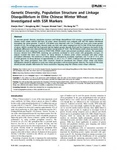
Figure 1: Ptype vs generations
0
50
100 Generations
150
Figure 2: Stddev vs generations
2
200
1
Gtype, PMX, Pc=0.7, Pm=0
0.9
0.8
0.8
0.7
0.7
0.6
0.6 Diversity
Diversity
1 0.9
0.5
0.5
0.4
0.4
0.3
0.3
0.2
0.2
0.1
0.1
0
0
50
100
150
0
200
Ancestral id, PMX, Pc=0.7, Pm=0
0
50
Generations
100
150
200
Generations
Figure 3: Gtypes vs generations
Figure 4: Uid vs generations
3 Diversity Measures Four diversity measures, namely the number of unique phenotypes, the fitness standard deviation, the total distance among genotypes, and the number of unique ancestral ids, are compared and studied in this paper. Phenotypes (ptype) The number of unique fitness values in the population, divided by size of the population. Standard deviation (stddev) The standard deviation of fitness values in a population: s 2 ∑N i=1 ( fi − f ) , stddev(P) = N −1
(2)
where N is the population size and f i is fitness of the ith individual.
Genotypes (gtype) The sum of the Hamming distances between any two genotypes(individual strings). The Hamming distance between genotype u and v is defined as: Hamming(u, v) = ∑ |sgn(u[i] − v[i])|,
(3)
i
where u[i] and v[i] are the ith gene (integer element) of the u and v, respectively. And the Hamming based population diversity of population P is thus: gtype(P) =
1 Hamming(P[i], P[ j])), 2 i6∑ =j
(4)
where P[i] and P[ j] are the ith and jth genotypes in P. We normalize gtype(P) by dividing it with (N 2 K)/2. Ancestral id (uid) Each individual in the initial population has a unique id. During crossover, two parents produce two children. One of the children inherits the mother’s uid and the other inherits the father’s uid. One’s uid changes when it’s mutated or being replaced in foreign talent procedure. 3
50
45
45
40
40
35
35 Mean Fitness Ranking
Mean Fitness Ranking
50
30 25 20
30 25 20
15
15
10
10
5
5
0
0
5
10
15
20
25
30
35
40
45
0
50
0
5
10
15
20
Diversity Ranking
50
50
45
45
40
40
35
35
30 25 20
10
5
5
15
20
25
45
50
20 15
10
40
25
10
5
35
30
15
0
30
Figure 6: Stddev rankings vs mean fitness rankings
Mean Fitness Ranking
Mean Fitness Ranking
Figure 5: Ptype rankings vs mean fitness rankings
0
25 Diversity Ranking
30
35
40
45
0
50
Diversity Ranking
Figure 7: Genotype rankings vs mean fitness rankings
0
5
10
15
20
25 30 Diversity Ranking
35
40
45
50
Figure 8: Uid rankings vs mean fitness rankings
The default crossover operator is PMX. The default initial population is a fixed, 100% random population. Our basic algorithm was run 10 times with the parameters: p c = 0.7, pm = 0 and p f = 0. In each generation, the population diversity is recorded by four measures defined above. Fig. 1 through Fig. 4 demonstrate the natural evolution of these measures over 201 generations. Phenotype measure displays a steep descent at about the 100th generation and quickly converges to close to zero. Genotype and standard deviation decrease more gradually, although stddev shows greater volatility. One can observe that the ptype diversity does not drop until the stddev and gtype diversities have decreased to almost zero. We may thus deduce that drop in stddev and gtype are the precursors to population convergence. The gradual descent of gtype measure also suggests this measure can be more useful in early prediction and diversity control. The rapid convergence of uid suggests that, with no mutation, the number of ids will monotonically decrease. The tendency of picking the fitter parents in selection causes the weaker ids to disappear very soon. The consistency of the four diversity measures can be estimated by taking the standard deviation of the average diversity over 50 runs. The standard deviations are σ ptype = 0.0814, σgtype = 0.0431, σstddev = 0.0445, and σuid = 0.0063. Stddev measure values were normalized to 1 before the calculation. Gtype and stddev measures appear more consistent than ptype. We ran the algorithm to 201 generations for 50 times, and plot the rankings of accumulated diversity over 201 generations against the rankings of the mean fitness at the 201st generation, for 4
every diversity measure in Fig. 5 through Fig. 8. Some moderate, positive correlation can be seen from all plots but uid, namely, the more diverse the populations are in a run, the better the search quality. The correlation is more evident in less consistent measures such as ptype and stddev. 1
Pc=0.3 Pc=0.4 Pc=0.5 Pc=0.6 Pc=0.7 Pc=0.8 Pc=0.9
2.5 Mean Standard Deviation Diversity
0.8
Mean Phenotype Diversity
3
Pc=0.3 Pc=0.4 Pc=0.5 Pc=0.6 Pc=0.7 Pc=0.8 Pc=0.9
0.9
0.7 0.6 0.5 0.4 0.3 0.2
2
1.5
1
0.5
0.1 0
0
50
100
150
0
200
0
50
Generations
Figure 9: Effect of PMX on Ptype 1
0.8
Pm=0.00 Pm=0.05 Pm=0.10 Pm=0.15 Pm=0.20 Pm=0.25 Pm=0.30
0.9 0.8 0.7 Mean Uid Diversity
Mean Genotype Diversity
200
Figure 10: Effect of PMX on Stddev
0.7 0.6 0.5 0.4
0.6 0.5 0.4
0.3
0.3
0.2
0.2
0.1
0.1
0
150
1
Pc=0.3 Pc=0.4 Pc=0.5 Pc=0.6 Pc=0.7 Pc=0.8 Pc=0.9
0.9
100 Generations
0
50
100 Generations
150
0
200
Figure 11: Effect of PMX on Gtype
0
50
100 Generations
150
200
Figure 12: Effect of mutation on Uid
4 Effects of Genetic Operators on Diversity Measures We hope to control the diversity through the three common genetic operators discussed in Section 2. Three sets of experiments were first conducted to demonstrate the independent effect of crossover, mutation and foreign talent on diversity. Crossover: pc = 0.3 · · ·0.9 (PMX), pm = 0, p f = 0 at step of 0.1. Mutation: pc = 0.4 (PMX) , pm = 0 · · ·0.30, p f = 0 at step of 0.05. Foreign talent: pc = 0.4 (PMX), pm = 0, p f = 0.1 · · ·0.4 at step of 0.1. Each set of parameters were tested 10 times and the mean diversity at each of the 201 generations was recorded by all four measures. We then plot the convergence graph for each diversity measure under different parameter settings, and these are included in Fig. 9 through Fig. 19. Uid diversity is only effected by mutation and foreign talent as only these two operators contribute new ids into the system, therefore a plot of crossover effect on uid is not included. One can observe from these plots that all three operators promote diversity by all measures. By increasing crossover rate pc , the gradient of descent does not change much. Instead the descent 5
1
Pm=0.00 Pm=0.05 Pm=0.10 Pm=0.15 Pm=0.20 Pm=0.25 Pm=0.30
2.5 Mean Standard Deviation Diversity
0.8
Mean Phenotype Diversity
3
Pm=0.00 Pm=0.05 Pm=0.10 Pm=0.15 Pm=0.20 Pm=0.25 Pm=0.30
0.9
0.7 0.6 0.5 0.4 0.3 0.2
2
1.5
1
0.5
0.1 0
0
50
100
150
0
200
0
50
Generations
Figure 13: Effect of mutation on Ptype 1
0.8
1
200
Pf=0.0 Pf=0.1 Pf=0.2 Pf=0.3 Pf=0.4
0.9 0.8 0.7 Mean Uid Diversity
0.7 Mean Genotype Diversity
150
Figure 14: Effect of mutation on Stddev
Pm=0.00 Pm=0.05 Pm=0.10 Pm=0.15 Pm=0.20 Pm=0.25 Pm=0.30
0.9
0.6 0.5 0.4
0.6 0.5 0.4
0.3
0.3
0.2
0.2
0.1
0.1
0
100 Generations
0
50
100
150
0
200
0
50
Generations
100
150
200
Generations
Figure 15: Effect of mutation on Gtype
Figure 16: Effect of foreign talent on Uid
is in general postponed, which is particularly evident in ptype and stddev measures. A growing mutation rate, on the other hand, exerts greater force of diversification right from the start. This causes the lines in the plots to curve up in most cases. Foreign talent displays a similar behavior, only more effectively diverges the population, especially in the stddev measure. Fig. 20 shows the comparison among the three crossover operators. OX, PMX and CX are applied to random population at pc from 0.1 to 0.9, and the number of generations when the gtype diversity reaches 0.5 is recorded for each setting. Apparently, OX is the most effective in boosting diversity while CX is the least effective.
5 Adaptive Control and Progression We apply the following universal adaptive function on the rates of crossover, mutation or foreign talent to maintain diversity at a target level: p0 = max(pmin , min(pmax , p(1 +
ξ(dt − d) ))), d
(5)
where p is the current rate of genetic operations, p0 is the new rate in the next generation, d is the diversity of current population, dt is the target diversity, ξ is the control sensitivity, and pmin , pmax are the lower and upper bounds of the rate (0 and 1 in this paper). A small ξ means gradual change in the rate, and that also translates into slower fluctuation of the diversity, a phenomenon we call 6
1
7
Pf=0.0 Pf=0.1 Pf=0.2 Pf=0.3 Pf=0.4
0.9
Pf=0.0 Pf=0.1 Pf=0.2 Pf=0.3 Pf=0.4
6
Mean Standard Deviation Diversity
Mean Phenotype Diversity
0.8 0.7 0.6 0.5 0.4 0.3
5
4
3
2
0.2 1 0.1 0
0
50
100
150
0
200
0
50
100
Generations
Figure 17: Effect of foreign talent on Ptype 1
400
Cycle Crossover Partial Match Crossover Order Crossover
350 Generations for Which Gtype is Above 0.5
0.8 0.7 Mean Genotype Diversity
200
Figure 18: Effect of foreign talent on Stddev
Pf=0.0 Pf=0.1 Pf=0.2 Pf=0.3 Pf=0.4
0.9
0.6 0.5 0.4 0.3 0.2
300
250
200
150
100
50
0.1 0
150
Generations
0
50
100
150
0 0.1
200
0.2
0.3
0.4
0.5
0.6
0.7
0.8
0.9
1
Generations
Probability of Crossover
Figure 19: Effect of foreign talent on Gtype
Figure 20: Comparison of OX, PMX and CX
ripple effect (see Fig. 21). Preliminary results show that larger ripples produce the opportunity of hopping from one local optimum to another. For the remaining experiments, a mixed initial population of both random and good solutions is used. The good individuals are obtained from Push Forward Insertion Heuristic (PFIH) [14] and its 2-neighborhood. We will focus on the gtype diversity as it behaves most consistently and is easy to control. A mix of PMX and OX is used in crossover. The initial crossover and mutation rates are 0.8 and 0.1, respectively. The progression of the mean fitness at various target gtype levels is plotted and illustrated in Fig. 22. When diversity is maintained at low levels, the population converges rather monotonically. When target diversity rises above 0.5, the population mean fitness starts to fluctuate, although such fluctuation appears to converge with time. Because the mean fitness curve approximately portrays the search horizon, a hovering curve essentially represents the traversal across a terrain of peaks and valleys in the solution space. One can see that the gtype=0.5 curve in Fig. 22 corresponds to the ξ = 0.01 ripple line in Fig. 21. Fig. 22 also indicated that overly high diversity, e.g. dt ≥ 0.9, will just cause the search to stray into random arena and perhaps diverge altogether. We test-ran both the fixed parameter GA and the adaptive GA up to 500 generations, with target diversity dt = 0.5 and ξ = 0.01 on all 56 Solomon problems with mixed initial population. The average values of pc and pm in the adaptive experiments were used as the settings in the fixed parameter experiments. The average results are compared in Table 1. Clearly, with the right target diversity, our adaptive GA consistently outperforms fixed parameter GA’s in terms of the quality 7
1
75
sensitivity = 0.01 sensitivity = 0.05 sensitivity = 0.10
0.9
target gtype = 0.1 target gtype = 0.3 target gtype = 0.5 target gtype = 0.7 target gtype = 0.9
70 65
0.8
Mean Fitness
Mean Gtype Diversity
60 0.7
0.6
0.5
55 50 45 40
0.4 35 0.3
0.2
30
0
200
400
600
800
25
1000
Generations
0
200
400
600
800
1000
Generations
Figure 21: The Ripple effect at low sensitivities and dt = 0.5
Figure 22: Mean fitness progression under target diversities 0.1 - 0.9 at step 0.2(PMX)
of solutions. And finally, in Table 2, our best solutions for the 56 problems are compared with best known solutions by various heuristics in the literature. Our results remains very competitive, which indicates that adaptive population diversity control is an encouraging new technique in the genetic algorithm research. Category C1 C2 R1 R2 RC1 RC2
pc /pm Fixed Time 0.88/0.49 10/835.6 72 0.89/0.36 3/610.9 804 0.85/0.56 13.3/1263.4 131 0.84/0.48 3.2/1021.4 1288 0.85/0.57 13.1/1437.2 177 0.84/0.49 3.9/1249.7 765
Category Adaptive Time C1 10/828.9 80 C2 3/589.9 735 R1 12.8/1242.7 305 R2 3/1016.4 1308 RC1 13/1412.0 239 RC2 3.7/1201.2 883
Table 1: Fixed parameter vs. adaptive algorithm (route/cost)
References [1] Allen L. Barker and Worthy N. Martin. Dynamics of a distance-based population diversity measure. In Proceedings of the 2000 Congress on Evolutionary Computation, pages 1002– 1009, Piscataway, NJ, 2000. IEEE Service Center. [2] Mark A. Bedau, Martin Zwick, and Alan Bahm. Variance and uncertainty measures of population diversity dynamics. Advances in Systems Science and Applications Special Issue, I:7–12, 1995. [3] Olli Br¨aysy and Wout Dullaert. A fast evolutionary metaheuristic for the vehicle routing problem with time windows. International Journal of Artificial Intelligence Tools, 12(2), 2002.
8
Prob. C1 C2 R1 R2 RC1 RC2
Best ever a 10/828.4 3/589.9 11.9/1228.1 2.7/961.3 11.5/1395.1 3.3/1139.4
I1b GIDEON c GEN d HG1/2 e DAGA f 10/951.9 10/892.1 10/838 10/828.4 10/828.9 3.1/692.7 3.0/749.1 3/590 3/589.9 3/589.9 13.6/1436.7 12.8/1300.3 12.6/1296.8 11.9/1228 12.8/1242.7 3.3/1402.4 3.2/1124.7 3/1117.7 2.7/970.0 3/1016.4 13.5/1596.5 12.5/1474.1 12.1/1446.2 11.6/1392.6 13/1412.0 3.9/1682.1 3.4/1411.1 3.4/1360.6 3.3/1144.4 3.7/1201.2
a Best
published: From [3] [14] 24-63 secs on DEC-10, 1 run. c GIDEON: [15] 2 mins on Solbourne 5/802, runs unknown. d GENEROUS: [13] 4-41 mins on SPARC 10, runs unknown e HG1/HG2: [9] 13-19 mins on Pentium 200MHz, 10 runs. f DAGA: Our diversity-controlling adaptive GA, 1-21 mins on Pentium 4 2.4GHz, 5 runs. b I1:
Table 2: Average of the best results in each category against the best known [4] Edmund Burke, Steven Gustafson, and Graham Kendall. A survey and analysis of diversity measures in genetic programming. In GECCO 2002: Proceedings of the Genetic and Evolutionary Computation Conference, pages 716–723. Morgan Kaufmann Publishers, 2002. [5] Matt Glickman and Katia Sycara. Reasons for premature convergence of self-adapting mutation rates. In Proc. of the 2000 Congress on Evolutionary Computation, pages 62–69, Piscataway, NJ, 2000. IEEE Service Center. [6] David E. Goldberg. Genetic Algorithms in Search, Optimization and Machine Learning. Addison-Wesley Pub. Co., 1989. [7] David E. Goldberg and Mike Rudnick. Genetic algorithm and the variance of fitness. Complex Systems, 5(3):265–278, 1991. [8] Francisco Herrera and Manuel Lozano. Adaptation of genetic algorithm parameters based on fuzzy logic controllers. Genetic Algorithms and Soft Computing, pages 95–125, 1996. [9] J¨org Homberger and Hermann Gehring. Two evolutionary meta-heuristics for the vehicle routing problem with time windows. INFORMS Jorunal on Computing, 37(3):297–318, 1999. [10] Samir W. Mahfoud. Crowding and preselection revisited. In Reinhard M¨anner and Bernard Manderick, editors, Parallel problem solving from nature 2, pages 27–36, Amsterdam, 1992. North-Holland. [11] Nicholas Freitag McPhee and Nicholas J. Hopper. Analysis of genetic diversity through population history. In GECCO99: Proceedings of the Genetic and Evolutionary Computation Conference, 1999.
9
[12] Ronald W. Morrison and Kenneth A. De Jong. Measurement of population diversity. In 5th International Conference, Evolution Artificielle, EA 2001, Le Creusot, France, Selected Papers, pages 31–41. Springer, 2001. [13] Jean-Yves Potvin and Samy Bengio. The vehicle routing problem with time windows - part ii: Genetic search. INFORMS Journal on Computing, 8:165–172, 1996. [14] Marius M. Solomon. Algorithms for vehicle routing and scheduling problems with time window constraints. Operations Research, 35(2), 1987. [15] S. R. Thangiah, K. E. Nygard, and P. L. Juell. Gideon: A genetic algorithm system for vehicle routing with time windows. In Proceedings of the Seventh Conference on Artificial Intelligence Applications, pages 322–325, 1991. [16] Kenny Q. Zhu. A diversity-controlling adaptive genetic algorithm for the vehicle routing pr oblem with time windows. In Proceedings of the 15th International Conference on Tools with Artificial Intelligence (ICTAI 2003). IEEE, 2003.
10