IJAESAM manuscript No. (will be inserted by the editor)
Pore–scale modeling and simulation of flow, transport, and adsorptive or osmotic effects in membranes: the influence of membrane microstructure V. M. Calo · O. Iliev∗ · Z. Lakdawala · K. H. L. Leonard · G. Printsypar
Received: date / Accepted: date
Abstract The selection of an appropriate membrane for a particular application is a complex and expensive process. Computational modeling can significantly aid membrane researchers and manufacturers in this process. The membrane morphology is highly influential on its efficiency within several applications, but is often overlooked in simulation. Two such applications which are very important in the provision of clean water are forward osmosis and filtration using functionalized micro/ultra/nano–filtration membranes. Herein, we investigate the effect of the membrane morphology in these two applications. First we present results of the separation process using resolved finger– and sponge–like support layers. Second, we represent the functionalization of a typical microfiltration membrane using absorptive pore walls, and illustrate the effect of different microstructures on the reactive process. Such numerical modeling will aid manufacturers in optimizing operating conditions and designing efficient membranes. Keywords Membrane · Microstructure · Pore–scale simulation · Surface reactions · Forward osmosis
1 Introduction The membrane microstructure significantly influences the membrane performance, due to its impact on the local flow rate, the pressure drop, and the filtration/separation efficiency. A common practice is to select or to develop membranes based on experimental evaluation. This is an expensive procedure requiring a prototype. Mathematical modeling and computer simulation is a powerful tool that can simplify the selection process. Numerical modeling provides information on quantities that cannot be measured experimentally, such as the local velocity field, and numerical experiments can also be performed, leading to a significant reduction in the number of required experiments in the laboratory. The combination of numerical modeling and experimental validation could aid membrane researchers and manufacturers in designing better membranes, tailored to specific applications. Our aim is to understand and quantify the influence of the membrane microstructure on the water (or other fluid) treatment efficiency, by describing the processes of interest at the pore–scale. This contrasts with the majority of theoretical studies which are performed at the Darcy scale (see, for example, [9, V. M. Calo AMCS, ErSE, Numerical Porous Media SRI Center, King Abdullah University of Science and Technology, Kingdom of Saudi Arabia. O. Iliev Fraunhofer Institute for Industrial Mathematics ITWM, Kaiserslatuern, Germany. E-mail:
[email protected] Numerical Porous Media SRI Center, King Abdullah University of Science and Technology, Kingdom of Saudi Arabia. · Z. Lakdawala DHI-WASY GmbH, Berlin, Germany. K. H. L. Leonard Fraunhofer Institute for Industrial Mathematics ITWM, Kaiserslatuern, Germany. G. Printsypar Numerical Porous Media SRI Center, King Abdullah University of Science and Technology, Kingdom of Saudi Arabia. * denotes corresponding author
z
Draw channel ICP
ECP
Selective layer Js
Jw
Support layer Feed channel
ECP
c Fig. 1 Concentration distribution in a forward osmosis (FO) mode with the selective layer facing the draw solution. The black line indicates the concentration polarization (CP) curve, comprising the external concentration polarization (ECP) and the internal concentration polarization (ICP), while c is the concentration, z is the vertical coordinate, and Jw and Js are the water and solute fluxes respectively
12, 26] for forward osmosis (FO) applications and [6, 17, 28] for reactive transport). A detailed pore– scale description of the processes yields more accurate results than a Darcy scale description, but at a higher computational cost. To the authors knowledge there are no pore–scale simulation studies on osmotic effects in membranes. Furthermore, although numerical studies on surface reactions at the pore– scale do exist, these are limited to pore–network models [24, 29] and, as far as we are aware, there are no software packages with the ability to solve surface reactions directly on images [14]. In contrast, our studies aim to examine the influence of the membrane morphology at the microscale directly on images obtained through techniques such as micro computerized tomography, or on virtually generated geometries when such images do not exist. In this paper we present illustrative numerical results to demonstrate the capability of the simulation tool that we are developing for two important applications in water filtration. Ongoing work will use these tools to predict the performance of different types of membrane microstructure on the performance, with the aim of improving the membrane efficiency. We first describe the mathematical models, before outlining the procedure used to numerically solve the systems of equations, and finally presenting results. The two applications areas we consider are the separation of solutes from water using FO [9, 25], and the removal of contaminants from water using micro/ultra/nano–filtration with functionalized membranes [7, 20]. Membranes for forward osmosis. In this work we first examine membranes for FO, which are essential components of desalination processes and have a number of other applications such as water purification and wastewater treatment [9]. In FO, water moves from a low to a high solute concentration due to an osmotic pressure gradient. The membranes used in FO usually consist of at least two layers, namely a selective layer and a support layer. The main function of the thin selective layer is to reject the solute, while the supporting layer acts as a base and provides mechanical support for the selective layer. The characteristics of both layers significantly influence the performance of the membrane and quantitatively predicting their effect will help improve the performance of the membrane. The most influential characteristics include the following: the water permeability of the selective and support layers as well as the solute rejection of the selective layer [27]; the concentration polarization (CP) [9, 21], namely external and internal concentration polarization, ECP and ICP, respectively; and membrane fouling. In this work we study the concentration polarization and in particular how it is influenced by the morphology of the supporting layer. A schematic representation of the ECP and ICP is shown in Figure 1 along with the concentration distribution for a membrane with a selective layer facing the feed channel in the FO mode. Membranes for micro/ultra/nano filtration. The second application considered in this work is water filtration using functionalized membranes. Clean water is essential for human health, and the supplies of water free from contaminants are not sufficient in many areas of the world [13]. Consequently, the purification of water and the removal of contaminants from waste water to prevent pollution of groundwater supplies or to allow reuse of the water, is an active area of research [23]. One method of achieving this is through the use of functionalization of membranes, which is a recent approach enabling efficient removal of impurities, such as bacteria and viruses. The process of functionalization involves chemically altering 2
the internal surfaces of the membrane so that particular pollutants are adsorbed. The functionalization may be achieved by processing the membrane, for example by plasma treatment, or by the addition of specific functional groups [20]. Among the membranes currently used in water filtration and purification, functionalized membranes are characterized by a larger pore–size [8], allowing a lower operating pressure and hence reducing energy consumption. Functionalized membranes are characterized as microfiltration, ultrafiltration or nanofiltration membranes depending on the size of the pores, and consequently our numerical model is applicable to all these types of membranes, although we present results on a geometry of a functionalized microfiltration membrane for illustrative purposes. Although, from the technical point of view, these two applications are different, the underlying mathematical models are similar with the computational simulation sharing common steps, enabling us to present them together. Our system of equations comprise the Navier–Stokes–Brinkman model for the fluid flow, coupled to a convection–diffusion equation for the solute/contaminant transport [18]. The difference in the mathematical description of the two processes enters through additional features; to account for osmotic effects in membranes used for the FO. We represent the selective layer as a zero–thickness interface and implement interfacial jump conditions, while for the contaminant removal in functionalized membranes we adopt an adsorptive boundary condition for the convection–diffusion equation at the pore walls. The construction of the computational model and its solution proceeds as follows. 3D computerized tomography (CT) or scanning electron microscopy (SEM) images are taken of membrane samples, and through image analysis, a 3D pore–scale geometry of a portion of the membrane is extracted directly. The fluid flow and transport of the species under consideration (solute or contaminants) at the pore–scale is then computed in a customized software tool. In this paper we use Pore–Chem, a Fraunhofer Institute for Industrial Mathematics (ITWM) in–house software package which is under development, and for which further details on the reactive flow may be found in [14]. Validation of the segmentation procedure may be performed by comparing the numerically evaluated membrane permeability and efficiency to the equivalent experimentally measured quantities. In a separate step, a virtual material design software tool, such as GeoDict [1], is used to analyze the characteristics of the 3D membrane geometry, such as porosity, pore–size distribution and tortuosity of the different layers comprising the membrane. From this analysis a virtual membrane is generated. The process of virtually generating the membrane may be validated by comparing the numerical results for the fluid flow and species transport computed on the 3D geometry obtained directly from the images to those computed on the virtual geometry. An iterative procedure may then be undertaken, whereby the results obtained from the pore–scale simulation are used to guide the manipulation of the membrane geometry, for which the fluid flow and species transport can then be recomputed and the results fed back into the virtual membrane geometry design. For this process to work, it is important that the software tool used can generate the virtual membrane microstructures by varying different characteristics (e.g., the same porosity, but different pore–size distribution). In this manner, the performance of the virtual membranes can be evaluated, and membrane scientists and engineers can be provided with relevant trends on the impact of the different modifications on the membrane performance. For example, how changes in the material used, pore–size, pore configuration and tortuosity can improve the performance. In many cases, however, a 3D geometry of the real membrane cannot be directly obtained, either because the imaging technique does not have enough resolution or because the equipment required is not available. In these cases a virtual membrane matching the statistical characteristics of the real membrane microstructure, which may be evaluated experimentally, must be generated. This is the method used in this paper. The remainder of the paper is structured as follows. The mathematical model, describing the conservation of mass and momentum, is presented in Section 2. In Section 3 we discuss the numerical discretization procedure employed, before presenting an illustrative and instructive example how a microstructure for a sponge type membrane can be generated in Section 4. In Section 5 we present the numerical experiments performed for the both applications. Finally, we draw some conclusions in Section 6.
2 Mathematical model Let us denote the computational domain of interest by Ω, which consists of three non–overlapping subdomains: a solid domain, Ωs , a porous domain, Ωp , and a free fluid region, Ωf , with Ω = Ωf ∪Ωs ∪Ωp . The boundary of the domain, ∂Ω, is decomposed into three different regions. We denote the inlet and 3
Γ in
Γw
Γ in
Ωf
Ωf
Γw
Γi
Γw
Γ out Ωs Γs
Γw Ωs
Ωf
Ωf
Ωp
Γs
Γ in
Γ out a.
Γw Counter–current cross flow setup
b.
Γ out Dead–end flow setup
Fig. 2 Typical filtration setups in a. cross–flow and b. dead–end configurations with the arrows indicate the direction of the flow at the inlets and outlets. The gray material represents the resolved portions of the solid membrane, while the blue material represents the portions of the membrane that are modeled as a porous medium, with the remaining volume of the computational domain representing the fluid region
outlet boundaries by Γ in and Γ out respectively, and represent the solid walls by Γ w , where ∂Ω = Γ w ∪ Γ in ∪ Γ out . Two typical filtration setups are cross flow and dead end. In a cross–flow setup the upper channel has a draw solution and the lower channel has a feed solution, with the fluid flowing tangentially to the membrane along the channels in either co– or counter–current directions (see Figure 2 a.). In a dead–end setup, as illustrated in Figure 2 b., all of the feed is forced through the membrane, which can result in a filtration–cake developing. Within this paper, we use a cross–flow setup for the osmotic applications and a dead–end setup for the functionalized membrane application, although both setups may be used for both applications. The pore–size distribution of water purification membranes often varies significantly in space. In this case one may wish to resolve the spatial microstructure of the large pores, while treating the portions of the membrane with smaller pores as a homogenized porous medium, resulting in a computational domain decomposed into porous parts, solid parts and fluid parts. In this case, we model the pore walls of the homogenized porous domain as permeable, with the pore walls of the resolved solid domain as impermeable. Such a setup is illustrated in Figure 2 a. with the blue regions representing Ωp (with permeable pore walls), while the gray regions represent Ωs (the solid walls are impermeable). The internal boundary of the solid domain is denoted by Γ s = Ωs ∩ (Ωf ∪ Ωp ) and is assumed to be impermeable. In contrast, if all the pores have a similar spatial scale, we may consider a fully resolved membrane structure. In this case Γ s = Ωs ∩ Ωf is impermeable and the porous domain is empty; such a situation is illustrated in Figure 2 b. For FO applications the membrane usually consists of two layers; a support layer and a selective layer. As the selective layer is very thin, we model this as a zero–thickness interface between the membrane and the draw channel, which we denote by Γ i , as shown in Figure 2 a. Assuming our fluid is Newtonian, the flow is laminar and incompressible, and the process is isothermal, there exist different models for simulating free fluid flow coupled with flow in porous media. One of the popular approaches is to use Stokes and Darcy flow problems with interface coupling conditions (see [22] and reference therein). Another approach is to use the Navier–Stokes–Brinkman model that was presented for the fluid flow through a filter element in [10] and references therein, which is the approach 4
we use here. For this model the system of equations for the flow is given by ρ
∂u + (ρu, ∇) u − ∇ · (µeff ∇u) + µK−1 u = −∇p, ∂t ∇ · u = 0,
x ∈ Ω \ Ωs ,
t ∈ [0, T ],
(1)
x ∈ Ω \ Ωs ,
t ∈ [0, T ],
(2)
where u and p denote the fluid velocity in [m/s] and pressure in [Pa] respectively, with t representing the time measured in [s] and T being the experimental end point measured in [s]. Moreover, µ and µeff are the fluid dynamic viscosity and the effective viscosity measured in [Pa s], K is the intrinsic permeability of the porous medium in Ωp and K−1 = 0 for x ∈ Ωf . Our boundary conditions are given by [10, 19] u(t, x) = uin (x),
x ∈ Γ in ,
σ · n = 0,
x∈Γ
out
x∈ Γ
u(t, x) = 0,
w
, s
∪Γ ,
t ∈ [0, T ],
(3)
t ∈ [0, T ],
(4)
t ∈ [0, T ],
(5)
where σ is the fluid stress tensor, n is the outward pointing unit normal to ∂Ω, and uin is the inflow velocity at the inflow boundary Γ in . By using the boundary condition (5) we assume that the fluid has no slip with respect to the solid surface. Although we employ no–flux and no–slip boundary conditions on Γ w , resulting in zero velocity being imposed on the portions of the external boundaries of the computational domain that are not inlets or outlets, periodic or symmetric boundary conditions can also be considered. These will be employed in our future work. Finally we need to prescribe initial conditions for the velocity and pressure. We use the initial conditions given by u(t = 0, x) = u0 (x),
x ∈ Ω \ Ωs ,
p(t = 0, x) = p0 (x),
x ∈ Ω \ Ωs .
The solute transport is modeled using the following convection–diffusion equation ∂c − ∇ · (D∇c) + ∇ · (uc) = 0, ∂t
x ∈ Ω \ Ωs ,
t ∈ [0, T ],
(6)
where c denotes the solute concentration measured in [M]. The diffusion coefficient, D, measured in [m2 /s] can take different scalar values in Ωf and in Ωp . In Ωf it is equal to the molecular diffusion of solute in the liquid, while in Ωp it is the effective diffusivity in porous media. The solute transport equation is supplemented by the following boundary conditions c(t, x) = cin , ∇c · n = 0, −D∇c · n = 0,
x ∈ Γ in ,
t ∈ [0, T ],
(7)
out
t ∈ [0, T ], t ∈ [0, T ],
(8) (9)
x∈Γ , x ∈ Γ w,
where n is the outward unit normal vector to corresponding boundary. The use of zero–flux boundary conditions in (9) is appropriate when no–flux conditions for the flow are employed on Γ w , as imposed through (5). If periodic or symmetric boundary conditions are imposed for the flow on Γ w then the corresponding boundary conditions for the solute transport would also be required. The initial condition for the solute concentration is prescribed through c (t = 0, x) = 0,
x ∈ Ω \ Ωs .
(10)
The system of equations for the flow model (1) – (5) and the mass transport model (6) – (9) need to be supplemented by appropriate boundary conditions for the internal boundary to the solid domain, Γ s , and interfacial jump conditions for selective layer, Γ i . We discuss additional boundary and interfacial conditions required separately for the two applications under consideration in the following sections. 5
2.1 Forward osmosis The selective layer is approximated by a zero–thickness layer, which is modeled as an interface condition between the free fluid region and the supporting layer. The interface is denoted by Γ i (see Figure 2 a.). We introduce an operator [f ]Γ i which indicates a jump of a function f across the interface Γ i [f ]Γ i =
lim
x→Γ i +0
f (x) −
lim
x→Γ i −0
f (x).
(11)
Then, to model the selective layer we impose the following interfacial conditions A ([p]Γ i − φ[π]Γ i ) , µd = −B[c]Γ i ,
[u(x) · n]Γ i = −
(12)
[Js (x) · n]Γ i
(13)
where Js = −D∇c + uc is the solute flux in [M m/s], A ([m2 ]) and B ([m/s]) are the water and solute permeability of the selective layer respectively, d is the thickness of the selective layer in [m], φ ([−]) is the reflection coefficient and π is the osmotic pressure in [kPa], which depends on the concentration. In addition, we impose no flux of the concentration at the internal solid boundary, so that −D∇c · n = 0,
x ∈ Γ s,
t ∈ [0, T ].
(14)
2.2 Functionalized membranes In order to account for the reactions that occur at the boundary Γ s , we assume that the change in adsorbed surface concentration is equal to the flux across the surface, so that ∂m = −D∇c · n, ∂t
x ∈ Γ s,
t ∈ [0, T ],
(15)
where m is the surface concentration of adsorbed pollutant in [M m] [16]. Assuming that there is a kinetic barrier at the reactive surface (for example due to conformational changes accompanying the adsorption of molecules), which effects the rate of adsorption, we may represent the change in surface concentration by the Henry isotherm ∂m = kads c − kdes m, ∂t
x ∈ Γ s,
t ∈ [0, T ].
(16)
Here kads is the rate of adsorption, measured in [m/s], and kdes is the rate of desorption, measured in [1/s]. These rates may be measured experimentally or via molecular dynamics [15]. A number of isotherms exist in literature to characterize different adsorption and desorption behaviors [5], of which the Henry isotherm is the simplest due to the linear dependence of the adsorption and desorption on c and m, repetitively. These other isotherms are discussed briefly in the conclusion. Although here we examine a purely pore–scale description for the surface reactions in the functionalized membrane application, and consider a fully resolved computational domain decomposed into either solid or fluid, so that Ωp = ∅, it is also possible, as in the FO applications, to consider porous portions of the computational domain. In this case F in (6) would be nonzero and describe the homogenized surface reactions, evaluated within a unit cell. Several studies have focused on rigorously determining the correct form of F from the pore–scale equations, for example [2–4]. However, due to the limited studies focusing on pore–scale surface reactions, we restrict ourselves here to considering surface reactions within a resolved solid and fluid domain. 6
3 Discretization The mathematical model is implemented within an in–house software tool called Pore–Chem. Before presenting the numerical results for the two separate applications under consideration, we briefly summarize the numerical methods and algorithms employed here, and direct the reader to [14] and references within for a more detailed description of the space and time discretization. The 3D computational geometry is discretized using a voxel grid. For both applications, FO and functionalized membranes, we begin by solving the fluid flow system of equations. A fractional timestep discretization is performed on the temporal derivative in (1), and the resultant spatial problem, along with the boundary conditions (3) – (5), at each timestep is discretized using the cell–centered finite volume method. The algorithm used to solve the discretized system of equations is detailed in [10, 18] and resembles a Chorin type fractional timestepping method.
For both the numerical experiments, we
∂u
proceed through time until steady–state is achieved and
ρ ∂t < tol, to give the velocity and pressure solutions, ust and pst . To solve the convection–diffusion equation (6) along with the associated boundary and interfacial conditions, given by (7) – (9) and either (12) – (14) or (15) – (16) depending on the application, we use a cell–centered finite volume method where the temporal derivatives are discretized by the implicit Euler method. In the reactive transport experiment considered here in connection with functionalized membranes, the geometry does not change throughout time, and the species concentration does not influence the flow. These two facts result in a one–way coupling between the flow and the species transport. Therefore, once the steady state flow is computed, it is used as input and we are required to solve (6) with u = ust along with the boundary condition (7) – (9), (15) and (16). This is achieved by, at each timestep, first solving (6) with (7) – (9) and (15), followed by (16), before time is updated. This is repeated until the experimental endpoint is reached. In contrast, there is a two–way coupling between the Navier–Stokes–Brinkman and the convection– diffusion systems of equations for the FO experiment, due to the dependence of the interfacial conditions (12) and (13) on the velocity, pressure and solute concentration. In general, the algorithms discussed here are developed to allow an investigation of two cases: (i) the temporal evolution of the concentration, the velocity and the pressure fields, and (ii) the spatial distributions of the solute concentration, pressure and velocity at steady state. In the computational experiments presented in Section 5.1 we are interested in the steady–state of the coupled system, thus time becomes an iterative parameter and ust and pst along with (10) become the initial conditions. We proceed by solving first the convection–diffusion system for n timesteps, where n is a non–zero integer, before the fluid flow This is repeated until
is recomputed.
∂u ∂c
steady–state for both the flow and efficiency is achieved, where ρ < tol and < tol. The smaller ∂t ∂t the choice of n the more accurate the numerical solution but the higher the computational burden; in our simulations presented below we choose n = 3 which shows good compromise between accuracy and computational costs.
4 Generation of virtual microstructures Before proceeding to generate a virtual membrane, the real membrane first needs to be characterized. The porosity and the permeability of the real membrane are determined using laboratory experiments, and the thickness of the membrane, pore–size, pore shape, and pore distribution are estimated from SEM images. Using this information, virtual 3D membranes with resolved morphology are generated using the software tool GeoDict [1]. In order to illustrate how this is performed, we now discuss the generation of a virtual sponge membrane in detail, which consists of three main steps. First, we generated large pores represented by spheres as shown in Figure 3 on the left. These spheres represent the pores and are assumed to be empty space. Small ellipsoids with centers uniformly distributed everywhere except for in the spheres are then generated as shown in the middle Figure 3. The last step is to put a binder between the ellipsoids, which is shown as the red substance in Figure 3 on the right. The resultant virtual geometry is shown in Figure 4 and corresponding SEM images of the real membrane along with its characterization can be found in [27]. 7
Fig. 3 Generation steps of the virtual sponge. In the first step spheres are generated which then become void space (left hand side). In a second step ellipsoids are generated (middle picture) before a binder is added, as illustrated in red on the right hand side picture
5 Numerical experiments 5.1 Forward osmosis experiment Based on data from media characterization, along with SEM images and laboratory measurements of porosity and water permeability, we can virtually generate the 3D morphology of different support layers. Here we consider two different types of support structures, sponge–like and finger–like supports, produced at the Water Desalination and Reuse Center at the King Abdullah University of Science and Technology (KAUST). More details on the membranes and their characterization can be found in [27]. The software tool GeoDict [1] is used to generate the virtual morphologies, in a similar manner to that outlined in Section 4, and the resulting structures are shown in Figures 4 and 5. To illustrate the effect of the morphology on the distributions of the solute concentration, pressure and velocity, we present results from three numerical experiments with the same input parameters but different support layers as follows: – Sponge-like membrane with fully resolved geometry; – Finger-like membrane with impermeable walls; – Finger-like membrane with porous walls. The numerical results at steady–state for the solute concentration (left–hand side), velocity (middle) and pressure (right–hand side) are presented in Figures 6 – 8 for the three test cases. The position of the ICP in the solute concentration may clearly be seen in each of the support layers, in a similar manner to that indicated in Figure 1. The simulation results also yield the ECP distribution in the draw and feed channels, as well as the spatial distribution of the water and solute fluxes in the selective layer (not shown). Shallow washing near the feed channel, at the base of the membrane as illustrated, may be observed in the velocity distributions in the middle of Figures 6 – 8. We note that the position of the ICP, and the spatial distribution of the solute concentration, is different in each of the support layers examined. This indicates that each support layer will give a different performance due to the distinct microstructures.
5.2 Functionalized membranes experiment Experimental measurements of the porosity and permeability of a commercially available microfiltration polyvinylidene fluoride membrane with a nominal pore–size of 0.2 microns, of which an SEM image may be found in [11], were performed. Using this information and assuming that the membrane is isotropic and symmetric, we generate two separate 3D virtual membranes with the aim of representing the membrane morphology. These virtual membranes are labeled membranes A and B and are illustrated in Figure 9. The virtual generation is performed using the software tool GeoDict [1], in a similar manner to the 8
Fig. 4 Virtually generated structures of sponge–like support layer for the FO application
Fig. 5 Virtually generated structures of finger–like support layer for the FO application
Fig. 6 Distributions of solute concentration, velocity, and pressure from left to right for the sponge–like support layer for the FO application
Fig. 7 Distributions of solute concentration, velocity, and pressure from left to right for the finger–like support layer with impermeable pore walls for the FO application
9
Fig. 8 Distributions of solute concentration, velocity, and pressure from left to right for the finger–like support layer with porous walls for the FO application
Fig. 9 Two virtually generated membranes for the reactive transport application with similar properties to a commercially available polyvinylidene fluoride microfiltration membrane with a nominal pore–size of 0.2 microns, of which SEM images may be found in [11]
method described in Section 4. Although the resultant microstructures have the same macroscopic characteristics, such as porosity and permeability, due to the different parameters used for their generation, the microscopic characteristics, such as the pore–size distribution and surface area, of the membranes A and B are different. The results from the flow experiments are presented in Figure 10. Due to the one–way coupling between the fluid flow and the contaminant transport system of equations, the velocity and pressure solutions remain constant through time. The efficiency results at three separate time points are shown in Figures 11 and 12 for the fluid phase and solid phase concentrations respectively. As time progresses, there is an increase in the adsorbed concentration at the pore wall, as shown in Figure 12. This, by the conservation of mass, results in a decrease in the fluid concentration as time progresses, as may be seen in Figure 11, with a larger decrease towards the outlet (bottom of the membrane here) than at the top of the membrane due to the constant contaminant concentration at the inlet. Due to the linear dependence of the rate of adsorption on c in (16), the lower concentration of contaminant in the fluid towards the outlet results in a lower adsorbed concentration than at the inlet, with the effect increasing with time, as may be seen in Figure 12. Examination of how the number of adsorbed particles of the contaminant 10
evolves with time in Figure 13 illustrates an almost linear increase in the total adsorbed number of particles in both membranes, with more particles being captured in virtual membrane A than in virtual membrane B although identical parameters for the fluid flow, contaminant transport and reaction are used. The difference in the predicted performance is due to the different microscopic characteristics, such as pore–size distribution and surface area, of the geometries describing Membranes A and B, which have a direct influence on the adsorption dynamics. This demonstrates the importance of pore–scale simulations.
Fig. 10 Distributions of the velocity (left) and pressure (right) for the virtually generated membranes A (top row) and B (bottom row) for the reactive transport application
6 Conclusions Purification of water for human consumption and use is of immense importance. The use of membranes to perform this task, removing contaminants and pollutants or unwanted solutes from water, is becoming increasingly prevalent. Numerical modeling of the processes involved can simplify the process of designing new membranes and modules, with the aim of increasing efficiency while reducing energy and material consumption. The focus of this work is on the numerical modeling of the processes involved in two separate water purification applications, where the use of membranes is extensive; firstly for forward osmosis, and 11
Fig. 11 Fluid concentration of the pollutant at three separate time points for the reactive transport application. The top row shows results computed on Membrane A whereas the bottom row shows results computed on Membrane B. The corresponding results for the adsorbed concentration at the solid–fluid interface are shown in Figure 12
secondly in functionalized membranes. For both applications, we present numerical results for the performance of virtually generated membranes with resolved microstructures at the pore–scale to illustrate the capabilities of the simulation tool, Pore–Chem, that we are developing. By examining the processes at the pore–scale, we demonstrate the effect of the membrane morphology on the predicted membrane efficiency. For FO, the mathematical model accounts for the osmotic effect across the selective layer. Two separate types of support layer, sponge–like and finger–like, are virtually generated based on images of real membranes which were produced in Water Desalination and Reuse Center in KAUST [27]. Three numerical simulations for FO on the sponge–like support, the finger–like support with impermeable walls, and the finger–like support with porous walls are presented. These results illustrate the influence of different support layers on the water flux through the selective layer under the same operational conditions and make evident the importance of considering a pore–scale representation in numerical experiments. We then present illustrative results for reactive transport in functionalized virtual membranes, constructed to model a commercially available microfiltration membrane. The two virtually generated membranes, although sharing similar characteristics, exhibit different pressure and velocity distributions, due to differences in the local velocity fields and internal surface area. This results in the quantity of pollutant being captured over the time period of the experiment being higher under membrane A than membrane B. In particular, as the velocity and pressure distributions influence the capturing kinetics, the imposed flow rate will have a large influence on the efficiency of the membrane. The mathematical model and numerical methods presented could be used to optimize the flow rate, module design, and calculate when is best to replace or chemically clean the membrane, so as to provide optimal removal of containments with minimal energy consumption. In this work we have used the Henry isotherm to characterize the adsorption kinetics, which assumes a linear relationship for the rate of adsorption and desorption. More sophisticated isotherms exist, for example the Langmuir isotherm, for which the rate of adsorption also depends on the quantity of material already adsorbed [16]. Such an isotherm would be suitable for cases where the number of adsorption sites is limited. 12
Fig. 12 Adsorbed concentration of the pollutant at the fluid–solid interface at three separate time points for the reactive transport application. The top row shows results computed on Membrane A whereas the bottom row shows results computed on Membrane B. The corresponding results for the fluid concentration are shown in Figure 11 17
Number of particles adsorbed
4
x 10
3.5 3
Membrane A Membrane B
2.5 2 1.5 1 0.5 0 0
2
4 6 Time (seconds)
8
10
Fig. 13 Number of particles of the pollutant adsorbed at the fluid–solid interface versus time, for the two virtually generated membranes under consideration for the reactive transport application
The numerical experiments presented in this paper illustrate the influence of the membrane microstructure on the predicted efficiency of the membrane. Using mathematical modeling and numerical simulation of the processes within the membrane microstructure at the pore–scale can lead to significant improvements in membrane design and technology. Ongoing and future work will include the implementation of more physically–realistic boundary conditions and the comparison of numerical and experimental results Acknowledgements We would like to thank Prof. Suzana Nunes and Meixia Shi from Water Desalination and Reuse Center in KAUST for providing the SEM images, information about the membranes, and input parameters for the FO experiments, and for the fruitful discussions. In addition we thank Emanuele Di Nicol` o from Solvay Specialty Polymers for helpful and informative discussions on the microfiltration membranes used as inspiration for the reactive transport experiments.
13
References 1. The virtual material laboratory geodict. http://www.geodict.com. 2014 2. Allaire, G., Brizzi, R., Mikeli´ c, A., Piatnitski, A.: Two-scale expansion with drift approach to the Taylor dispersion for reactive transport through porous media. Chemical Engineering Science 65(7), 2292–2300 (2010). DOI 10.1016/j.ces. 2009.09.010 3. Allaire, G., Hutridurga, H.: Homogenization of reactive flows in porous media and competition between bulk and surface diffusion. IMA Journal of Applied Mathematics 77(6), 788–815 (2012). DOI 10.1093/imamat/hxs049 4. Allaire, G., Mikeli´ c, A., Piatnitski, A.: Homogenization approach to the dispersion theory for reactive transport through porous media. Society of Industrial and Applied Mathematics Journal on Mathematical Analysis 42(1), 125–144 (2010). DOI 10.1137/090754935 5. Baret, J.F.: Theoretical model for an interface allowing a kinetic study of adsorption. Journal of Colloid and Interface Science 30(1), 1–12 (1969). DOI 10.1016/0021-9797(69)90373-7 6. Bhattacharjee, S., Ryan, J.N., Elimelech, M.: Virus transport in physically and geochemically heterogeneous subsurface porous media. Journal of Contaminant Hydrology 57(3-4), 161–187 (2002). DOI 10.1016/s0169-7722(02)00007-4 7. der Bruggen, B.V.: Removal of pollutants from surface water and groundwater by nanofiltration: overview of possible applications in the drinking water industry. Environmental Pollution 122(3), 435–445 (2003) 8. Bruggen, B.V.D., Vandecasteele, C., Gestel, T.V., Doyen, W., Leysen, R.: A review of pressure-driven membrane processes in wastewater treatment and drinking water production. Environ. Prog. 22(1), 46–56 (2003). DOI 10.1002/ ep.670220116 9. Cath, T., Childress, A., Elimelech, M.: Forward osmosis: Principles, applications, and recent developments. J. Membr. Sci. 281(1–2), 70–87 (2006) 10. Ciegis, R., Iliev, O., Lakdawala, Z.: On parallel numerical algorithms for simulating industrial filtration problems. Berichte des Fraunhofer ITWM (114) (2007) 11. Di Nicol` o, E., Iliev, O., Leonard, K.: Virtual generation of microfiltration membrane geometry for the numerical simulation of contaminent transport. Tech. Rep. 245, Fraunhofer-Institut f¨ ur Techno- und Wirtschaftsmathematik ITWM (2015) 12. Gruber, M., Johnson, C., Tang, C., Jensen, M., Yde, L., H´ elix-Nielsen, C.: Validation and analysis of forward osmosis CFD model in complex 3D geometries. J. Membranes 2, 764–782 (2012) 13. Hunter, P.R., MacDonald, A.M., Carter, R.C.: Water Supply and Health. PLoS Med 7(11), e1000,361+ (2010) 14. Iliev, O., Lakdawala, Z., Leonard, K.H.L., Vutov, Y.: On pore–scale modeling and simulation of reactive transport in 3D geometries. Submitted to Advances in Water Resources (2015) 15. Kang, H.C., Weinberg, W.H.: Modeling the Kinetics of Heterogeneous Catalysis. Chemical Reviews 95(3), 667–676 (1995). DOI 10.1021/cr00035a010 16. Kralchevsky, P.A., Danov, K.D., Denkov, N.D.: Handbook of Surface and Colloid Chemistry, Third Edition, chap. Chemical Physics of Colloid Systems and Interfaces. Taylor & Francis (2008) 17. Kuhnen, F., Barmettler, K., Bhattacharjee, S., Elimelech, M., Kretzschmar, R.: Transport of Iron Oxide Colloids in Packed Quartz Sand Media: Monolayer and Multilayer Deposition. Journal of Colloid and Interface Science 231(1), 32–41 (2000). DOI 10.1006/jcis.2000.7097 18. Lakdawala, Z.: On efficient algorithms for filtration related multiscale problems. Ph.D. thesis, University of Kaiserslautern (2010) 19. Laptev, V.: Numerical solution of coupled flow in plain and porous media. PhD thesis, Technical University Kaiserslautern (2004) 20. Liu, F., Hashim, N.A., Liu, Y., Abed, M.R.M., Li, K.: Progress in the production and modification of PVDF membranes. Journal of Membrane Science 375(1-2), 1–27 (2011) 21. McCutcheon, J., Elimelech, M.: Influence of concentrative and dilutive internal concentration polarization on flux behavior in forward osmosis. J. Membr. Sci. 284, 237–247 (2006) 22. Mosthaf, K., Baber, K., Flemisch, B., Helmig, R., Leijnse, A., Rybak, I., Wohlmuth, B.: A coupling concept for twophase compositional porous-medium and single-phase compositional free flow. Water Resources Research 47, 1–19 (2011) 23. Pendergast, M.M., Hoek, M.V.: A review of water treatment membrane nanotechnologies. Energy Environ. Sci. 4(6), 1946–1971 (2011) 24. Raoof, A., Hassanizadeh, S.M., Leijnse, A.: Upscaling transport of adsorbing solutes in porous media: Pore–network modeling. Vadose Zone Journal 9, 624–636 (2010). DOI 10.2136/vzj2010.0026 25. Sablani, S., Goosen, M., Al-Belushi, R., Wilf, M.: Concentration polarization in ultrafiltration and reverse osmosis: a critical review. Desalination 141(3), 269–289 (2001) 26. Sagiv, A., Zhu, A., Christofides, P., Cohen, Y., Semiat, R.: Analysis of forward osmosis desalination via two-dimensional fem model. J. Membr. Sci. 464, 161–172 (2014) 27. Shi, M., Printsypar, G., Iliev, O., Calo, V., Amy, G., Nunes, S.: Water flow prediction based on 3-d membrane morphology simulation. J. Membr. Sci. 487, 19–31 (2015) 28. Sim, Y., Chrysikopoulos, C.V.: Virus transport in unsaturated porous media. Water Resources Research 36(1), 173–179 (2000). DOI 10.1029/1999wr900302 29. Varloteaux, C., Vu, M.T., B´ ekri, S., Adler, P.M.: Reactive transport in porous media: pore-network model approach compared to pore-scale model. Physical Review E: Statistical, Nonlinear, and Soft Matter Physics 87(2) (2013). DOI http://dx.doi.org/10.1103/PhysRevE.87.023010
14