Carl Lindberg ... Nielsen and Shephard type, to appear in Mathematical .... stochastic volatility framework of Barndorff$Nielsen and Shephard that the cen$.
Thesis for the Degree of Doctor of Philosophy
Portfolio Optimization and Statistics in Stochastic Volatility Markets Carl Lindberg
Department of Mathematical Sciences Division of Mathematical Statistics Chalmers University of Technology and Göteborg University Göteborg, Sweden 2005
Portfolio optimization and statistics in stochastic volatility markets Carl Lindberg Department of Mathematical Sciences, Chalmers University of Technology and Göteborg University, Sweden Large …nancial portfolios often contain hundreds of stocks. The aim of this thesis is to …nd explicit optimal trading strategies that can be applied to portfolios of that size for di¤erent n-stock extensions of the model by Barndor¤-Nielsen and Shephard [3]. A main ambition is that the number of parameters in our models do not grow too fast as the number of stocks n grows. This is necessary to obtain stable parameter estimates when we …t the models to data, and n is relatively large. Stability over the parameter estimates is needed to obtain accurate estimates of the optimal strategies. Statistical methods for …tting the models to data are also given. The thesis consists of three papers. Paper I presents an n-stock extension to the model in [3] where the dependence between di¤erent stocks lies strictly in the volatility. The model is primarily intended for stocks that are dependent, but not too dependent, such as stocks from di¤erent branches of industry. We develop optimal portfolio theory for the model, and indicate how to do the statistical analysis. In Paper II we extend the model in Paper I further, to model stronger dependence. This is done by assuming that the di¤usion components of the stocks contain one Brownian motion that is unique for each stock, and a few Brownian motions that all stocks share. We then develop portfolio optimization theory for this extended model. Paper III presents statistical methods to estimate the model in [3] from data. The model in Paper II is also considered. It is shown that we can divide the centered returns by a constant times the daily number of trades to get normalized returns that are i:i:d: and N (0; 1) : It is a key feature of the Barndor¤-Nielsen and Shephard model that the centered returns divided by the volatility are also i:i:d: and N (0; 1) : This suggests that we identify the daily number of trades with the volatility, and model the number of trades within the framework of Barndor¤-Nielsen and Shephard. Our approach is easier to implement than the quadratic variation method, requires much less data, and gives stable parameter estimates. A statistical analysis is done which shows that the model …ts the data well. Key words: Stochastic control, portfolio optimization, veri…cation theorem, Feynman-Kac formula, stochastic volatility, non-Gaussian Ornstein-Uhlenbeck process, estimation, number of trades iii
This thesis consists of the following papers: Paper I: News-generated dependence and optimal portfolios for n stocks in a market of Barndor¤-Nielsen and Shephard type, to appear in Mathematical Finance. Paper II: Portfolio optimization and a factor model in a stochastic volatility market, submitted. Paper III: The estimation of a stochastic volatility model based on the number of trades, submitted.
v
Contents 1
Introduction
1
2
Portfolio optimization
2
3
"Stylized" features of stock returns
4
4
Stochastic volatility models in …nance
4
5
Summary of papers 5.1 Paper I 5.2 Paper II 5.3 Paper III
7 7 8 8
Paper I Paper II Paper III
vii
Acknowledgements First of all I would like to thank my supervisors Holger Rootzén and Fred Espen Benth. They have both, in di¤erent ways, been of great help to me with their advice, constructive criticism, and encouragement. These years at the Department of Mathematical Sciences would not have been as fun and productive without my good friend and o¢ ce roommate Erik Brodin. I have bene…tted a lot from being able to discuss matters of research and life with him. I am grateful to my friends and colleagues at the Department of Mathematical Sciences for providing a pleasant working environment. I dedicate this thesis to my friends and family, who make my life great. Especially My wonderful parents Ewa and Lars-Håkan, and sisters Kristina and Anna, for their unconditional love and support. My beloved sons Adam and Bo, for constantly reminding me of what is important in life. My best friend, …ancée, and mistress Cia. I love you.
ix
1
Introduction
Investing in the stock market can be a pain free way to get rich fast. All you have to do is to buy the right stock at the right time for a lot of money that you don’t necessarily have to own. However, no one knows what "the right stock" or "the right time" is, except in retrospective. Fortunately, the humble investor can …nd other, more feasible, goals than "to get rich fast." For example, a trader can try to maximize her expected utility from investing. The concept of utility is an attempt to capture the risk aversion of a trader: The more money a trader has, the less interested she will be in an extra 100SEK: The idea of portfolio optimization is natural. A trader has a certain amount of money and wants to invest it in a way that maximizes her expected utility. In other words, she wants to do what she feels is best for her on average. In fact, there is nothing about this optimality condition that is speci…c to …nance. The optimal allocation of capital to di¤erent assets is a fundamental problem in …nance. The …rst contribution to the area was by Markowitz [19]. He suggested that an investor should consider not only the expected rate of return of the stocks, but also the amount of ‡uctuation, or volatility, of the stock prices. This lead to optimal portfolios that diversi…ed the capital between di¤erent assets, instead of investing all the money in the stock with the highest mean rate of return. Later, Merton solved related problems in continuous time in [20] and [21]. Merton assumed that stocks behave as multi-variate geometric Brownian motions. This implies that the volatilities are constant. The geometric Brownian motion is the classic stock price model in stochastic …nance. It is a well-known empirical fact that many characteristics of stock price data are not captured by the geometric Brownian motion, and many alternatives have been proposed. A successful approach that captures several key features of …nancial data was presented by Barndor¤-Nielsen and Shephard in [3]. They suggested a stochastic volatility model based on linear combinations of OrnsteinUhlenbeck processes with dynamics dy =
y (t) dt + dz (t) ;
where z is a subordinator and > 0: A subordinator is a Lévy process with increasing paths. This framework allows us to model several of the observed features in …nancial time series, such as semi-heavy tails, volatility clustering, and skewness. Further, it is analytically tractable, see for example [2], [4], [7], [22], and [24]. We consider some n-stock extensions of this model. Large …nancial portfolios often contain hundreds of stocks. The aim of this thesis is to …nd explicit optimal trading strategies that can be applied to portfolios of that size for di¤erent n-stock extensions of the model in [3]. A primary objective is that the number of parameters in our models do not grow too fast as the number of stocks n grows. This is necessary to obtain stable parameter estimates when we …t the models to data, and n is relatively large. Stability over the parameter estimates is needed to obtain accurate estimates of the optimal strategies. We also give statistical methods for …tting the models to data.
1
Paper I presents an n-stock extension to the Barndor¤-Nielsen and Shephard model where the dependence between di¤erent stocks lies in that they partly share the Ornstein-Uhlenbeck processes of the volatility. The model is mainly intended for stocks that are dependent, but not too dependent, such as stocks that are not in the same branch of industry. We develop portfolio optimization portfolio theory, and indicate how to do the statistical analysis for the model. In Paper II we extend the model in Paper I further, so that it can model stronger dependence between di¤erent stocks. This is done by introducing a factor structure in the di¤usion components. The idea of a factor structure is that the di¤usion components of the stocks contain one Brownian motion that is unique for each stock, and a few Brownian motions that all stocks share. We then develop optimal portfolio theory for this extended model. Paper III presents statistical methods to estimate the model in [3] from data. We also consider the model from Paper II. It is shown that we can divide the centered returns by a constant times the daily number of trades to get normalized returns that are i:i:d: and N (0; 1) : It is an important theoretical feature of the stochastic volatility framework of Barndor¤-Nielsen and Shephard that the centered returns divided by the volatility are also i:i:d: and N (0; 1) : This suggests that we identify the daily number of trades with the volatility, and model the number of trades within the framework of Barndor¤-Nielsen and Shephard. Our approach gives more stable parameter estimates than if we analyzed only the marginal distribution of the returns directly with the standard maximum likelihood approach. Further, it is easier to implement than the quadratic variation method, and requires much less data. A statistical analysis is done which shows that the model …ts the data well. In Section 2 of this summary we recapitulate some results from classical continuous time portfolio optimization, and the ideas from stochastic control used to derive them. Section 3 discusses "stylized" facts of stock price data. Further, we indicate why the classical models lack all these characteristics. Section 4 introduces the stochastic volatility model of [3]. Finally, in Section 5 we present the three papers that constitute this thesis.
2
Portfolio optimization
The …rst papers on continuous time portfolio optimization are due to Merton ([20] and [21]). We present in this section a version of Merton’s problem in its classical setting. Merton modelled the stock prices as multi-variate geometric Brownian motions, which for two stocks S1 ; S2 takes the form S1 (t) = S1 (0) exp (
1
S2 (t) = S2 (0) exp (
2
1 2 2 11 1 2 2 21
1 2 2 12 )t 1 2 2 22 )t
+
11 W1
(t) +
12 W2
(t) ;
+
21 W1
(t) +
22 W2
(t) :
(2.1)
Here i ; i = 1; 2; are constants, Wi ; i = 1; 2; are independent Brownian motions, and is a volatility matrix. The matrix gives the dependence between the two stocks. 2
In portfolio optimization one has to choose a value function to optimize. One of the most widely used optimal value functions is V (t; w) = sup E [U (W (T )) jt; W (t) = w ] ; where T is a future date in time, W (T ) is our wealth at time T , U ( ) is our utility function, and is a trading strategy. The utility function is a measure of how much we want to risk to obtain more wealth. It is typically assumed to be concave and increasing. The concavity means that the more money an investor gets, the less interested she will be in obtaining a little more. The condition that the utility function should be increasing implies that the investor always prefers more to less. Merton suggested the utility function U (w) =
1
w ;
for 0 < < 1: The trading strategies are recipes for how we are going to allocate our wealth between di¤erent assets. This formulation of the portfolio optimization problem means that we seek the trading strategies such that we obtain the maximum expected utility from wealth on a future day T: We outline now the stochastic control approach to …nding this optimal value function V: First, one assumes that sup lim t#0
E [V (t; W (t))] t
V (0; w)
= 0:
This "derivative" serves as a necessary condition for optimality. It can be evaluated using Itô’s formula which gives an equation called the Hamilton-JacobiBellman (HJB) equation. So far, we have only found an equation whose solution we guess is the optimal value function. The next step is to prove a veri…cation theorem. This theorem says that a solution to the HJB-equation is in fact equal to the optimal value function. Hence, we have veri…ed that our guess was correct. The last and …nal step is then to actually …nd the solution to the HJB equation. This is typically quite hard, since the HJB-equation is nonlinear. However, it can be done in the setting of this section, and the optimal trading strategies turn out to be =(
0
)
1
(
r1) ¯ 1
1
;
where 1 is a vector of ones. ¯ Portfolio optimization with more general stock price models than the geometric Brownian motion has been treated in a number of recent articles. In [7], a one-stock portfolio problem in the model in [3] is solved. In the papers [13], [14], [23], and [26], the stochastic volatility depends on a Brownian motion which is correlated to the di¤usion process of the risky asset. The paper [9] model the volatility as a continuous-time Markov chain with …nite state-space, which is independent of the rest of the model. In [5], [6], and [12], di¤erent portfolio 3
problems are treated when the stocks are driven by general Lévy processes, and [10] look at portfolio optimization in a market with Markov-modulated drift process. Further, [15] derive explicit solutions for log-optimal portfolios in complete markets in terms of the semimartingale characteristics of the price process, and [18] show that there exists a unique solution to the optimal investment problem for any arbitrage-free model if and only if the utility function has asymptotic elasticity strictly less than one.
3
"Stylized" features of stock returns
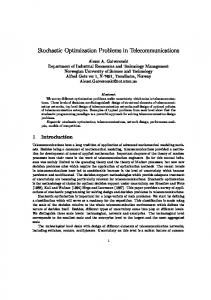
The standard approach to analyze …nancial data is to look at the increments of the returns process R (t) := log (S (t) =S (0)) for the stock S: We assume that we are observing returns R ( ) ; R (2 ) R ( ) ; :::; R (k ) R ((k 1) ) ; where is one day, and k+1 is the number of consecutive trading days in our period of observation. It is widely agreed that the returns of …nancial data have, among other things, the following characteristic features: The returns are not normally distributed. Instead, they are peaked around zero, skew, and have heavier tails than the normal distribution. The volatility of the returns changes stochastically over time, and appears to be clustered. That is, there seems to be a random succession of periods with high return variance and periods with low return variance. The autocorrelation function for absolute returns is clearly positive even for long lags. We now give a brief indication that these empirical facts hold. The empirical density function of the returns in Figure 3.1 seems consistent with the …rst listed feature. It shows a clear non-normality, and appears to be both peaked around zero, skew, and more heavy-tailed than the normal distribution. In Figure 3.2, the volatility of the returns is evidently not constant. The most obvious example of a volatility cluster is the latter part of 2002. Hence these data give no reason to doubt the second "stylized" fact. Further, the autocorrelation function of the absolute returns in Figure 3.3 is positive, and so appears compatible with the last condition. The stock price model in Equation (2.1), which is used in the classical portfolio optimization problem above, does not capture any of the features listed above: The returns in this model are i:i:d: and normally distributed, and the volatility is constant. A common approach to improve the geometric Brownian motion as a stock price model is to assume that the volatility is stochastic.
4
Stochastic volatility models in …nance
There has been published some di¤erent models that include stochastic volatility in stock price dynamics, see for example [3], [11], [16], and [17]. This thesis 4
25
20
15
10
5
0 -0.08
-0.06
-0.04
-0.02
0
0.02
0.04
0.06
0.08
Figure 3.1: Stars indicate the empirical density function for daily returns for Volvo B during 1999-08-16 to 2004-08-16. The solid line is the estimated normal density function to the same data set.
0.2
0.15
0.1
0.05
0
-0.05
-0.1
-0.15
-0.2
-0.25 1999-08-16
2002-02-06
2004-08-16
Figure 3.2: Returns for Ericsson from 1999-08-16 to 2004-08-16.
5
1
0.9
0.8
0.7
0.6
0.5
0.4
0.3
0.2
0.1
0 0
10
20
Figure 3.3: Empirical autocorrelation function for absolute returns for SKF from 1999-08-16 to 2004-08-16.
builds upon extensions of the model in [3]. In this model the volatility 2 ( ) of a stock is de…ned as a linear combination of non-Gaussian Ornstein-Uhlenbeck processes of the form Rt (4.1) Yj (t) = yj e j t + 0 e j (t u) dZj ( j u); t 0:
Here yj := Yj (0) ; and yj has the stationary marginal distribution of the process and is independent of Zj (t) Zj (0) ; t 0: The process Zj is a subordinator, that is, a Lévy process with positive increments. The stock price process S then takes the form Z t Z t 2 1 S (t) = S (0) exp + (u) du + (u) dW (u) ; 2 0
0
for some Brownian motion W: It can be shown that the returns in this model can get marginal distributions from the Generalized Hyperbolic (GH) distribution. The GH family is quite general, and includes many distributions that have been used to model …nancial return data, for example the normal inverse Gaussian (N IG) distribution, see [1], [3], and [25]. The use of subordinators allows for sudden increases in the volatility 2 ( ), which can be interpreted as the release of unexpected information. Further, since the Ornstein-Uhlenbeck processes Yj decrease exponentially, the e¤ect of large jumps in the volatility 2 ( ) "lingers." This models volatility clustering. In essence, the model captures all "stylized" facts of …nancial data listed above. A further advantage of the Barndor¤-Nielsen and Shephard model is that it is analytically tractable; Option pricing is treated 6
in [22], portfolio optimization for one stock and a bond in [7], and inference techniques are developed, for example, in [4] and [24].
5
Summary of papers
Most published papers on portfolio optimization with more general stock price models than the geometric Brownian motion consider only the case of one stock and a bond. However, large …nancial portfolios often contain hundreds of stocks. We want to develop explicit optimal trading strategies that can be applied to portfolios of this size for di¤erent n-stock extensions of the model in [3]. This requires careful modeling of the stock price and volatility dynamics. It is necessary to have many more observations than parameters to obtain stable parameter estimates. Therefore, we can not use the standard approach: An explicit stochastic volatility matrix, and n Brownian motions in the di¤usion components of all n stocks. The reason is that the number of parameters in such a model would grow very fast as the number of stocks grows. We want to capture the essence of the dependence between di¤erent stocks, but still be able to estimate the model accurately from data.
5.1
Paper I
In this paper we consider Merton’s portfolio optimization problem in a Barndor¤Nielsen and Shephard market. An investor is allowed to trade in n stocks and a risk-free bond, and wants to maximize her expected utility from wealth at the terminal date T . The case with only one stock was solved in [7]. The dependence between stocks is assumed to be that they partly share the Ornstein-Uhlenbeck processes of the volatility. We refer to these as news processes. This gives the interpretation that dependence between stocks lies solely in their reactions to the same news. The model is primarily intended for assets which are dependent, but not too dependent, such as stocks from di¤erent branches of industry. We show that this dependence generates covariance between the returns of di¤erent stocks, and give statistical methods for both the …tting and veri…cation of the model to data. The model retains all the features of the univariate model in [3]. The stochastic optimization problem is solved via dynamic programming and the associated HJB integro-di¤erential equation. By use of a veri…cation theorem, we identify the optimal expected utility from terminal wealth as the solution of a second-order integro-di¤erential equation. The investor is allowed to have restrictions on the fractions of wealth held in each stock, but also borrowing and short-selling constraints on the entire portfolio. For power utility, we then compute the solution to this equation via a Feynman-Kac representation, and obtain explicit optimal allocation strategies. A main advantage with the model is that the optimal strategies are functions of only 2n model parameters and the volatility of each stock. This is a desirable feature which allows us to obtain good estimates of the optimal strategies even when n is large. All results are derived under exponential integrability assumptions on the Lévy measures
7
of the subordinators.
5.2
Paper II
The model in Paper I has a weak point: To obtain strong correlations between the returns of di¤erent stocks, the marginal distributions have to be very skew. This might not …t data. In the …rst part of Paper II, we try to deal with this weakness. We introduce in Paper II a more general n-stock extension of the model in Paper I. It is a primary focus that the number of parameters does not grow too fast as the number of stocks grows. This is necessary to obtain accurate parameter estimates when we …t the model to data, and n is relatively large. Accurate parameter estimates is needed to obtain good estimates of the optimal strategies. Therefore, we do not use the standard approach with n Brownian motions in the di¤usion components of all n stocks. Instead, we de…ne the stochastic volatility matrix implicitly by a factor structure. The idea of a factor structure is that the di¤usion components of the stocks contain one Brownian motion that is unique for each stock, and a few Brownian motions that all stocks share. The latter are called factors. Hence, the dependence between stocks lies both in the stochastic volatility, and in the Brownian motions. A factor model has fewer parameters than a standard model. The reason is that the number of factors can be chosen a lot smaller than the number of stocks. We show that this model can obtain strong correlations between the returns of the stocks without a¤ecting their marginal distributions. In the second part we consider an investor who wants to maximize her utility from terminal wealth by investing in n stocks and a bond. We allow for the investor to have restrictions on the fractions of wealth held in each stock, as well as borrowing and short-selling restrictions on the entire portfolio. The stochastic optimization problem is solved via dynamic programming and the associated HJB integro-di¤erential equation. We use a veri…cation theorem to identify the optimal expected utility from terminal wealth as the solution of a second-order integro-di¤erential equation. We then compute the solution to this equation via a Feynman-Kac representation for power utility, and obtain explicit optimal allocation strategies. All results are derived under exponential integrability assumptions on the Lévy measures of the subordinators.
5.3
Paper III
A drawback with the Barndor¤-Nielsen and Shephard model has been the dif…culty to estimate the parameters of the model from data. Perhaps the most intuitive approach to do this is to analyze the quadratic variation of the stock price process, see [4]. This makes it in theory possible to recover the volatility process from observed stock prices. However, in reality the model does not hold on the microscale, and even if is only regarded as an approximation this approach still requires very much data. In addition, it is hard to implement in a statistically sound way due to peculiarities in intraday data. For example, 8
the stock market is closed at night, and there is more intense trading on certain hours of the day. None of these features are present in the mathematical model. In this paper we develop statistical methods for estimating the models in [3] and Paper II from data. The models are discretized under the assumption that the Wiener integrals in the Barndor¤-Nielsen and Shephard model Z t (s) dB (s) (t) "; t
for " 2 N (0; 1) : In addition, we impose some restrictions on the volatility in order to be able to estimate the model from data. We argue that it is inappropriate to estimate the GH-distribution directly from …nancial return data. The reason is that the GH-distribution is "almost" overparameterized. To overcome this problem, we verify that we can divide the centered returns by a constant times the number of trades in a trading day to get a sample that is i:i:d: and N (0; 1) : It is an important feature of the stochastic volatility framework in [3] that the centered returns divided by the volatility are also i:i:d: and N (0; 1) : This implies that we identify the daily number of trades with the volatility, and model the number of trades within the model in [3]. Our approach gives more stable parameter estimates than if we analyzed only the marginal distribution of the returns directly with the standard maximum likelihood method. Further, it is easier to implement than the quadratic variation method, and requires much less data. It gives also an economical interpretation of the discretely observed linear combination of non-Gaussian Ornstein-Uhlenbeck processes that de…ne the stochastic volatility. In addition, our approach implies that we can view the continuous time volatility as the intensity with which trades arrive. A statistical analysis is performed on data from the OMX Stockholmsbörsen. The results indicate a good model …t.
References [1] Barndor¤-Nielsen, O.E. (1998): Processes of normal inverse Gaussian type, Finance and Stochastics 2, 41-68. [2] Barndor¤-Nielsen, O. E., Shephard, N. (2001a): Modelling by Lévy processes for …nancial econometrics, in Lévy Processes - Theory and Applications (eds O. E. Barndor¤-Nielsen, T. Mikosch and S. Resnick). Boston: Birkhäuser. [3] Barndor¤-Nielsen, O. E., Shephard, N. (2001): Non-Gaussian OrnsteinUhlenbeck-based models and some of their uses in …nancial economics, Journal of the Royal Statistical Society: Series B 63, 167-241 (with discussion). [4] Barndor¤-Nielsen, O. E., Shephard, N. (2002): Econometric analysis of realized volatility and its use in estimating stochastic volatility models, Journal of the Royal Statistical Society: Series B 64, 253-280. 9
[5] Benth, F. E., Karlsen, K. H., Reikvam K. (2001a): Optimal portfolio selection with consumption and non-Linear integro-di¤erential equations with gradient constraint: A viscosity solution approach, Finance and Stochastics 5, 275-303. [6] Benth, F. E., Karlsen, K. H., Reikvam K. (2001b): Optimal portfolio management rules in a non-Gaussian market with durability and intertemporal substitution, Finance and Stochastics 5, 447-467. [7] Benth, F. E., Karlsen, K. H., Reikvam K. (2003): Merton’s portfolio optimization problem in a Black and Scholes market with non-Gaussian stochastic volatility of Ornstein-Uhlenbeck type, Mathematical Finance 13(2), 215-244. [8] Black, F., Scholes M. (1973): The pricing of options and corporate liabilities, Journal of Political Economy 81, 637-654. [9] Bäuerle, N., Rieder, U. (2004): Portfolio optimization with Markovmodulated stock prices and interest rates, IEEE Transactions on Automatic Control , Vol. 49, No. 3, 442-447. [10] Bäuerle, N., Rieder, U. (2005): Portfolio optimization with unobservable Markov-modulated drift process, to appear in Journal of Applied Probability. [11] Carr, P., Geman, H., Madan, D. B., Yor, M. (2003): Stochastic volatility for Lévy processes, Mathematical Finance 13(3), 345-382. [12] Emmer, S., Klüppelberg, C. (2004): Optimal portfolios when stock prices follow an exponential Lévy process, Finance and Stochastics 8, 17-44. [13] Fleming, W. H., Hernández-Hernández, D. (2003): An optimal consumption model with stochastic volatility, Finance and Stochastics 7, 245-262. [14] Fouque, J.-P., Papanicolaou, G., Sircar, K. R. (2000): Derivatives in Financial Markets with Stochastic Volatility. Cambridge: Cambridge University Press. [15] Goll, T., Kallsen, J. (2003): A complete explicit solution to the log-optimal portfolio problem, Annals of Applied Probability 13, 774-799. [16] Heston, S. (1993): A closed-form solution for options with stochastic volatility with applications to bond and currency options, Review of Financial Studies 6, 327-343. [17] Hull, J., White, A. (1987): The pricing of options on assets with stochastic volatilities, Journal of Finance 42, 281-300. [18] Kramkov, D., Schachermayer, W. (1999): The asymptotic elasticity of utility functions and optimal investment in incomplete markets, Annals of Applied Probability 9, 904-950. 10
[19] Markowitz H. (1952): Portfolio selection, Journal of Finance 7, 77-91. [20] Merton, R. (1969): Lifetime portfolio selection under uncertainty: The continuous time case, Review of economics and statistics 51, 247-257. [21] Merton, R. (1971): Optimum consumption and portfolio rules in a continuous time model, Journal of Economic Theory 3, 373-413; Erratum (1973) 6, 213-214. [22] Nicolato, E., Venardos, E. (2003): Option pricing in stochastic volatility models of the Ornstein-Uhlenbeck type, Mathematical Finance 13(4), 445466. [23] Pham, H., Quenez, M-C. (2001): Optimal portfolio in partially observed stochastic volatility models, Annals of Applied Probability 11, 210-238. [24] Roberts, G.O., Papaspiliopoulos, O., Dellaportas, P. (2004): Bayesian inference for non-Gaussian Ornstein-Uhlenbeck stochastic volatility processes, Journal of the Royal Statistical Society: Series B 66 (2), 369-393. [25] Rydberg, T. H. (1997): The normal inverse Gaussian Lévy process: Simulation and approximation, Communications in Statistics: Stochastic Models 13(4), 887-910. [26] Zariphopoulou, T. (2001): A solution approach to valuation with unhedgeable risks, Finance and Stochastics 5, 61-82.
11
News-generated dependence and optimal portfolios for n stocks in a market of Barndor¤-Nielsen and Shephard type Carl Lindberg Department of Mathematical Sciences, Chalmers University of Technology and Göteborg University, Sweden Abstract We consider Merton’s portfolio optimization problem in a Black and Scholes market with non-Gaussian stochastic volatility of Ornstein-Uhlenbeck type. The investor can trade in n stocks and a risk-free bond. We assume that the dependence between stocks lies in that they partly share the Ornstein-Uhlenbeck processes of the volatility. We refer to these as news processes, and interpret this as that dependence between stocks lies solely in their reactions to the same news. The model is primarily intended for assets which are dependent, but not too dependent, such as stocks from di¤erent branches of industry. We show that this dependence generates covariance, and give statistical methods for both the …tting and veri…cation of the model to data. Using dynamic programming, we derive and verify explicit trading strategies and Feynman-Kac representations of the value function for power utility. A primary advantage with the model is that the optimal strategies are functions of only 2n model parameters and the volatility of each stock. This allows us to obtain accurate estimates of the optimal strategies even when n is large.
1
Introduction
A classical problem in mathematical …nance is the question of how to optimally allocate capital between di¤erent assets. In a Black and Scholes market with constant coe¢ cients, this was solved by Merton in [16] and [17]. Recently, [6] solved a similar problem for one stock and a bond in the more general market model of [3]. In [3], Barndor¤-Nielsen and Shephard propose modeling the volatility in asset price dynamics as a weighted sum of non-Gaussian OrnsteinUhlenbeck (OU) processes of the form dy (t) =
y (t) dt + dz (t) ;
The author would like to thank Holger Rootzén and Fred Espen Benth for valuable discussions, as well as for carefully reading through preliminary versions of this paper.
1
where z is a subordinator and > 0. This framework is a powerful modeling tool that allows us to capture several of the observed features in …nancial time series, such as semi-heavy tails, volatility clustering, and skewness. We extend the model by introducing a new dependence structure, in which the dependence between assets lies in that they share some of the OU processes of the volatility. We will refer to the OU processes as news processes, which implies the interpretation that the dependence between …nancial assets is reactions to the same news. We show that this dependence generates covariance, and give statistical methods for both the …tting and veri…cation of the model to data. The model is primarily intended for assets which are not too dependent, such as stocks from di¤erent branches of industry. In this extended model we consider an investor who wants to maximize her utility from terminal wealth by investing in n stocks and a bond. This problem is an n-stock extension of [6]. We allow for the investor to have restrictions on the fractions of wealth held in each stock, as well as borrowing and short-selling restrictions on the entire portfolio. For simplicity of notation, we have formulated and solved the problem for two stocks and a bond. However, the general case is completely analogous. The stochastic optimization problem is solved via dynamic programming and the associated Hamilton-Jakobi-Bellman (HJB) integro-di¤erential equation. By use of a veri…cation theorem, we identify the optimal expected utility from terminal wealth as the solution of a second-order integro-di¤erential equation. For power utility, we then compute the solution to this equation via a Feynman-Kac representation, and obtain explicit optimal allocation strategies. These strategies are functions of only 2n model parameters and the volatility of each stock. This is a desirable feature which allows us to do portfolio optimization with a large number of stocks. All results are derived under exponential integrability assumptions on the Lévy measures of the subordinators. Recently, portfolio optimization under stochastic volatility has been treated in a number of articles. In [11], [13], and [23], the stochastic volatility depends on a stochastic factor that is correlated to the di¤usion process of the risky asset. The paper [8] models the stochastic factor as a continuous-time Markov chain with …nite state-space. This process is assumed to be independent of the di¤usion process. Both [8] and [23] use an approach to solve their portfolio optimization problems that is similar to ours. The paper [19] uses partial observation to solve a portfolio problem with a stochastic volatility process driven by a Brownian motion correlated to the dynamics of the risky asset. Going beyond the classical geometric Brownian motion, [4], [5], and [10] treat di¤erent portfolio problems when the risky assets are driven by Lévy processes, and [9] look at portfolio optimization in a market with unobservable Markov-modulated drift process. Further, [14] derive explicit solutions for log-optimal portfolios in terms of the semimartingale characteristics of the price process. For an introduction to the market model of Barndor¤-Nielsen and Shephard we refer to [2] and [3]. For option pricing in this context, see [18]. This paper has six sections. In Section 2 we give a rigorous formulation of the market and the portfolio optimization problem. We also discuss the market 2
model and the implications of the dependence structure. In Section 3 we derive some useful results on the stochastic volatility model, and on moments of the wealth process. We prove our veri…cation theorem in Section 4, and use it in Section 5 to verify the solution we have obtained. Section 6 states our results, without proofs, in the general setting.
2
The optimization problem
In this section we de…ne, and discuss, the market model. We also set up our optimization problem.
2.1
The market model
For 0 t T < 1, we assume as given a complete probability space ( ; F; P ) with a …ltration fFt g0 t T satisfying the usual conditions. Introduce m independent subordinators Zj , and denote their Lévy measures by lj (dz); j = 1; :::; m: Remember that a subordinator is de…ned to be a Lévy process taking values in [0; 1) ; which implies that its sample paths are increasing. The Lévy measure l of a subordinator satis…es the condition Z 1 min(1; z)l(dz) < 1: 0+
We assume that we use the cádlág version of Zj : Let Bi ; i = 1; 2; be two Wiener processes independent of all the subordinators. We now introduce our stochastic volatility model. It is an extension of the model proposed by Barndor¤-Nielsen and Shephard in [3] to the case of two stocks, under a special dependence structure. To begin with, our model is identical to theirs. We will discuss the di¤erences as they occur. The next extension of the model, to n stocks, is only a matter of notation. Denote by Yj ; j = 1; :::; m, the OU stochastic processes whose dynamics are governed by dYj (t) = (2.1) j Yj (t)dt + dZj ( j t), where the rate of decay is denoted by j > 0: The unusual timing of Zj is chosen so that the marginal distribution of Yj will be unchanged regardless of the value of j : To make the OU processes and the Wiener processes simultaneously adapted, we use the …ltration f (B1 (t) ; B2 (t) ; Z1 (
1 t) ; :::; Zm
(
m t))g0 t T
:
From now on we view the processes Yj ; j = 1; :::; m in our model as news processes associated to certain events, and the jump times of Zj ; j = 1; :::; m as news or the release of information on the market. The stationary process Yj can be represented as Rt Yj (s) = 1 exp (u) dZj ( j s + u) ; s t; 3
but can also be written as Yj (s) = yj e
j (s
t)
+
Rs t
e
j (s
u)
dZj (
j u);
s
t;
(2.2)
where yj := Yj (t) ; and yj has the stationary marginal distribution of the process and is independent of Zj (s) Zj (t) ; s t: In particular, if yj = Yj (t) 0; then Yj (s) 0; since Zj is non-decreasing. We set Zj (0) = 0, j = 1; :::; m; and set y := (y1 ; :::; ym ) : We assume the usual risk-free bond dynamics dR (t) = rR (t) dt; with interest rate r > 0. De…ne the two stocks S1 ; S2 to have the dynamics p (2.3) dSi (t) = ( i + i i (t)) Si (t) dt + i (t)Si (t) dBi (t) . Here i are the constant mean rates of return; and i are skewness parameters. We will call i + i i (t) the mean rate of return for stock i at time t: For notational simplicity in our portfolio problem we denote the volatility processes by i instead of the more customary i2 : We de…ne i as Pm t;y (2.4) i (s) := i (s) := j=1 !i;j Yj (s) ; s 2 [t; T ] ; where !i;j 0 are weights summing to one for each i: The notation it;y denotes conditioning on Y (t) : Our model is here not the same as just two separate models of Barndor¤-Nielsen and Shephard type. The di¤erence is that the volatility processes depend on the same news processes. These volatility dynamics gives us the stock price processes Z sp Z s 1 (u) du + Si (s) = Si (t) exp + i (u)dBi (u) : (2.5) i i i 2 t
t
This stock price model does not have statistically independent increments and it is non-stationary. It also allows for the increments of the returns Ri (t) := log (Si (t) =Si (0)) ; i = 1; 2; to have semi-heavy tails as well as both volatility clustering and skewness. The increments of the returns Ri are stationary since Ri (s)
Ri (t) = log
Si (s) Si (0)
log
Si (t) Si (0)
= log
Si (s) Si (t)
=L Ri (s
t) ;
where " =L " denotes equality in law.
2.2
Discussion of the market model
This section aims to show that the dependence structure proposed in Section 2.1 is not only simple from a statistical point of view, but also has very appealing economical interpretations. The paper [3] suggests a model with n stocks with dynamics dS (t) = f +
(t)g S (t) dt + 4
1
(t) 2 S (t) dB(t);
where is a time-varying stochastic volatility matrix, and are vectors, and B is a vector of independent Wiener processes. This model includes ours as a special case with being a diagonal matrix. However, in the classical Black and Scholes market, dependence is modelled by covariance. In the case of two stocks this means that for s t; p p 1 1 S1 (s) = S1 (t) exp t) + 11 B1 (s) + 12 B2 (s) ; 1 2 11 2 12 (s and S2 (s) = S2 (t) exp
1 2 21
2
1 2 22
(s
t) +
p
21 B1
(s) +
p
22 B2
(s) ;
for a volatility matrix ; and B1 (t) = B2 (t) = 0. In our model, stock prices develop independently beside from reacting to the same news. The model is mainly intended for assets that are dependent, but not too dependent. For example, stocks from di¤erent branches of industry. From an economic viewpoint, one can expect the model parameters to be more stable than in the classical Black and Scholes market. For example, we do not require stability over expected rate of return. Instead we ask that every time the market is ”nervous”to a certain degree, i.e. for every speci…c value of the volatility i ; the mean rate of return i + i i will be the same. We can interpret this as that we only need stability in how the market reacts to news. Note that we do not make a distinction between good and bad news. As we will see, for the purpose of portfolio optimization we do not need to know the weights !i;j : More importantly, the model generates a non-diagonal covariance matrix for the increments of the returns over the same time period, which is the most frequently used measure of dependence in …nance. Since the returns have stationary increments, it is su¢ cient to show this result for Ri ; i = 1; 2: Note that we have Cov (R1 (s) R1 (t) ; R2 (u) R2 (v)) = Cov (R1 (s) ; R2 (u)) Cov (R1 (s) ; R2 (v)) Cov (R1 (t) ; R2 (u)) + Cov (R1 (t) ; R2 (v)) ; for s; t; u; v 2 [0; T ] : As will be shown below, for s; t 2 [0; T ] ; we have that Cov (R1 (s) ; R2 (t)) =
1 2
1
2
(2.6)
1 2
m X
!1;j !2;j V ar (Yj (0))
j=1
e
js
+e
jt
j js
e
tj
1+2
j
min (s; t)
2 j
;
which for s = t simpli…es to Cov (R1 (t) ; R2 (t)) =2
1
1 2
2
(2.7) 1 2
m X
!1;j !2;j V ar (Yj (0))
j=1
5
e
jt
1+ 2 j
jt
:
This result says that the model generates a covariance matrix between returns, but we do not immediately know which correlations that can be obtained. It turns out that we can get correlations Corr (R1 (t) ; R2 (t)) in the entire interval ( 1; 1) : To derive Equation (2.6), by de…nition of i we have that E [R1 (s) R2 (t)] Z s =E 1+
1 2
1
0
Z
2
+
1 2
2
1 2 st
+
1s
(u) du +
2 m X
1 2
2
+
2t
m X
1
!1;j E
j=1
+
1 2
1
m X
1 2
2
s
Z
p
1
Z tp
(u)dB1 (u)
2
(u)dB2 (u)
0
Z
!2;j E
t
Yj (u) du
0
j=1
1 2
Z
0
t
0
=
1 (u) du +
s
Yj (u) du
0
Z
!1;i !2;j E
s
Yi (u) du
0
i;j=1
Z
t
Yj (u) du :
0
Similarly, E [R1 (t)] =
1t +
1
m X
1 2
!1;j E
j=1
Z
t
Yj (u) du :
0
This gives that Cov (R1 (s) ; R2 (t)) =
1
1 2
1 2
2
m X
Z
!1;j !2;j Cov
s
Yj (u) du;
0
j=1
Z
t
Yj (u) du :
0
By stationarity, we have that E [Yj (t)] = Yj ; for some constant Yj > 0; for all t 2 R: If we assume that u v; the independence of the increments of Yj gives that Cov (Yj (u) ; Yj (v)) =E
Yj (u)
=e
j (v
=e
j (v
Yj (v)
Yj
Z v 2 Yj (u) + Yj (u) e j (v u h i 2 u) E Yj (0) e j (v u) 2Yj
j (v
=E e
Yj
u)
u)
s)
dZ (
j s)
V ar (Yj (0)) :
The same calculations for v
u shows that
Cov (Yj (u) ; Yj (v)) = e 6
j jv
uj
V ar (Yj (0)) ;
2 Yj
and we get Cov =
Z
Z
s
Yj (u) du;
0
s
Z
Z
t
Yj (u) du
(2.8)
0
t
Cov (Yj (u) ; Yj (v)) dudv
0
0
= V ar (Yj (0))
e
js
+e
jt
j js
e
tj
1+2
j
min (s; t)
2 j
:
By Itô’s isometry (see [24]) we get, similarly as above, V ar (Ri (t)) =
m X
2
i
1 2 2
2 !i;j V ar (Yj (0))
jt
e
1+
jt
2 j
j=1
+ !i;j
for i = 1; 2: This gives Corr (R1 (s) ; R2 (t)) =
1 2
1 2 1 2
1 1
e
1 2 1 2
2 2
js
+e
jt
m X
!1;j !2;j V ar (Yj (0))
j=1
e
j js
tj
1+2
j
min (s; t)
2 j
1
v u uPm t
j=1
js
1+
js
2 j
!1;j
+
2
1
Yj s 1 2
2
1
v u uPm t
j=1
and, for s = t;
2 V ar (Y (0)) !1;j j
e
2 V ar (Y (0)) !2;j j
e
jt
1+
jt
2 j
+
!2;j 2
2
Yj t
1 2
2
! !;
Corr (R1 (t) ; R2 (t)) =
1 2 1 1 2 m X
1
2 2
1 2 1 2
!1;j !2;j V ar (Yj (0))
jt
e
1+
j=1
v u uPm t
j=1
jt
2 j
1 2 V !1;j
ar (Yj (0))
7
e
jt
1+ 2 j
jt
+
!1;j 2
1
Yj t
1 2
2
!
Yj t
!
;
1
v u uPm t
j=1
2 V ar (Y (0)) !2;j j
e
jt
1+
jt
2 j
+
!2;j 2
2
Yj t 1 2 2
!:
There is always a trade-o¤ between accuracy and applicability when designing models. An obvious advantage of our model is that we do not have to estimate a stochastic volatility matrix, and hence we need less data to obtain good estimates of the model parameters. A drawback is that, to obtain high correlations, we need the model to be very skew. This might not …t observed data. Another drawback is that we do not distinguish between good and bad news. An alternative stock price model would be p 2 2 dSi (t) = i + i1 i1 (t) i (t)Si (t) dBi (t) , i i (t) Si (t) dt +
where i1 ; i2 > 0; and i1 ; i2 are linear combinations of the news processes such that i1 + i2 = i : We have chosen to not use this model as it would be hard to estimate from data. For example, the marginal distributions of the returns will no longer …t in the framework of Barndor¤-Nielsen and Shephard. We are also required to obtain estimates of the "positive" respectively "negative" volatilities in the statistical estimation of the model.
2.3
Statistical methodology
In this section we describe a methodology for …tting the model to return data. We will do this for a Normalized Inverse Gaussian distribution (N IG) ; which has been shown to …t …nancial data well, see e.g. [1], [3], and [21]. Our choice plays no formal role in the analysis. We assume that we are observing Ri ( ) ; Ri (2 ) Ri ( ) ; :::; Ri (k ) Ri ((k 1) ) ; where is one day, and k +1 is the number of consecutive trading days p in our period of observation. 2 + 2 ; ; ; and : Its density The N IG-distribution has parameters = function is fN IG (x; ; ; ; ) p 2 = exp
2
1
x
q
K1
x
q
e x;
p where q (x) = 1 + x2 and K1 denotes the modi…ed Bessel function of the third kind with index 1: The domain of the parameters is 2 R; ; > 0; and 0 j j : A standard result is that if we take to have an Inverse Gaussian distribution p " (IG) ; and draw a N (0; 1)-distributed random variable "; then x = + + will be N IG-distributed. The IG-distribution has density function fIG (x; ; ) =
p
2
exp (
)x
3 2
exp
1 2
2
x
1
+
2
x
;
x > 0;
where and are the same as in the N IG-distribution. The existence and integrability of Lévy measures lj such that the volatility processes i will have 8
IG-distributed marginals is not obvious. See [2] and [22] for this theory. The Lévy density l of the subordinator Z of an IG-distributed news process Y is l (x) = (2 )
1 2
2
x
1
+
2
x
1 2
e
2x 2
;
where ( ; ) are the parameters of the IG-distribution, see [3]. The method described in [3], which we further extend, uses that the marginal distributions of the volatility processes i are invariant to the rates of decay j : These parameters j are then used to …t the autocorrelation function of the i ; (h) = Cov ( i (h) ; i (0)) =V ar ( i (0)) ; h 2 R; to log-return data. i For simplicity of exposition we will assume that we only need one to correctly model the autocorrelation function of both stocks. However, for reasons to be explained later, we will assume that m = 3; and that all 1 = 2 = 3 = : For our model calculations show that, for general m; i
(h) = !i;1 exp (
1
jhj) + ::: + !i;m exp (
m
jhj) ;
where the !i;j 0; are the weights from the volatility processes that sum to one. Observe that since we have assumed the rates of decay j to be equal, we immediately get that i (h) = exp ( jhj) : We proved this simpler result in Subsection 2.2. The proof of the general case is analogous. We assume that we have …tted N IG-distributions to the empirical marginal distributions of two stocks, and that we have found a such that our model has the right autocorrelation function. This can be done by empirically calculating the autocorrelation functions i (h) for di¤erent values of h; and then …nd a so that the theoretical and empirical autocorrelation functions match. We denote the IG-parameters of the volatility processes i by ( i ; i ) ; i = 1; 2: By Equation (2.7) we can now …t the covariance of the model to the empirical covariance from the return data. This can be done by letting the two stocks ”share”the news process Y3 , and each have one of the news processes Yi ; i = 1; 2; ”of their own.”In general, this is done for each rate of decay. We formulate this mathematically as 1 2
= !1;1 Y1 + !1;3 Y3 = !2;1 Y2 + !2;3 Y3
IG ( 1 ; 1 ) IG ( 2 ; 2 ) :
We now state two properties of IG-distributed random variables that we will need below. For X IG ( X ; X ), we have that aX
1
IG a 2
X; a
1 2
X
:
Furthermore, if Y IG ( Y ; Y ) and is independent of X and we assume that IG ( X + Y ; ) : Because of this formula X = Y =: ; we have that X + Y we can let !1;1 Y1 IG ( 1;1 ; 1 ) !1;3 Y3 IG ( 1;3 ; 1 ) ;
9
where 1;1
+
1;3
=
1;
(2.9)
and !2;1 Y2 !2;3 Y3
IG ( 2;1 ; 2 ) IG ( 2;3 ; 2 ) ;
where 2;1
+
2;3
=
2;
(2.10)
We see, by the scaling property of the IG-distribution, that the two expressions for the distribution of Y3 , 1 2
1
Y3
IG !1;32
Y3
IG !2;32
and
1;3 ; !1;3 1
1
1 2
2;3 ; !2;3 2
;
(2.11)
;
(2.12)
must be identical. With the aid of Equation (2.8), in which we use that the variance V ar (Y (0)) of a stationary inverse Gaussian process Y is = 3 , we see that Equation (2.7) becomes 2
1
1 2
2
1 2
!1;3 !2;3
2;3 3 2
e
j
1+ 2 j
j
=C
(2.13)
where C is the covariance that we want the returns to have. It is now straightforward to check that for reasonably small C there are non-unique choices of !i;j such that we can obtain both the right autocorrelation function of i and a speci…c covariance for the returns. The autocorrelation function parameter is already correct by assumption, and we constructed the news processes Yj so that their marginal distribution would not depend on it. Hence we only have to take care of the covariance of the returns Ri . We do this by using Equations (2.9),..., (2.13). Note that there is nothing crucial in our choice of covariance as measure of dependence, nor does it matter how many di¤erent rates of decay we use. We now give a simple approach to determine how well our model captures the true covariance. We begin by …tting a marginal distribution to return data, thereby obtaining the parameters i and i ; i = 1; 2: Since we have that the return processes R R si ; i = 1; 2; are semimartingales, their quadratic variations, denoted by [ ] ; are t i (u) du; s t: That is, for a sequence of random partitions tending to the identity, we have Z s [log (Si =Si (t))] (s) = i (u) du; t
where convergence is uniformly on compacts in probability. This is a standard result in stochastic calculus. For each trading day we now empirically calculate the integrated volatility, that is, we calculate the quadratic variation of the observed returns over a trading day and, by the formula above, use that 10
as a constant approximation of the volatility during that day. If we do this for a number of trading days, we get approximations of the volatility processes i for that period of time. Using the …tted parameters i , i and generated N (0; 1)-distributed variables in Equation (2.5), we can now simulate ”alternative” returns. We then calculate the covariance-matrix of both the return data set and the simulated alternative returns and compare them statistically.
2.4
The control problem
A main purpose of this paper is to …nd trading strategies that optimizes the trader’s expected utility from wealth in a deterministic future point in time. The utility is measured by a utility function U chosen by the trader. This utility function U is a measure of the trader’s aversion towards risk, in that it concretizes how much the trader is willing to risk to obtain a certain level of wealth. Our approach to …nding these trading strategies, and the value function V , is dynamic programming and stochastic control. We will make use of many of the results in [6], since most of their ideas are applicable in our setting. However, we need to adapt their results to our case. In this section we set up the control problem under the stock price dynamics of Equation (2.3). Recall that 1 and 2 ; are weighted sums of the news processes, see Equation (2.4). We begin by de…ning a value function V as the maximum amount of expected utility that we can obtain from a trading strategy, given a certain amount of capital. We then set up the associated Hamilton-Jakobi-Bellman equation of the value function V: This equation is a central part of our problem, as it is, in a sense, an optimality condition. Most of the later sections will be devoted to …nding and verifying solutions to it. Denote by i (t) the fraction of wealth invested in stock i at time t, and set = ( 1 ; 2 ) : The fraction of wealth held in the risk-free asset is (1 1 2 ). We allow no short-selling of stocks or bond, which implies the conditions i 2 [0; 1] ; i = 1; 2; and 1 + 2 1; a.s., for all t s T: However, these restrictions are partly for mathematical convenience. We could equally well have chosen constants ai ; bi ; c; d 2 R; ai < bi ; c < d; such that the constraints would have taken the form i 2 [ai ; bi ] ; i = 1; 2; and c d; a.s., for all t 1 + 2 s T: The analysis is analogous in this case, but more notationally complex. This general setting allows us to consider, for example, law enforced restrictions on the fraction of wealth held in a speci…c stock, as well as short-selling and borrowing of capital. We state the main results in this setting in Section 6. The wealth process W is de…ned as W (s) =
1
(s) W (s) S1 (s)+ S1 (s)
2
(s) W (s) (1 S2 (s)+ S2 (s)
1
(s) 2 (s)) W (s) R (s) ; R (s)
where i (s) W (s) =Si (s) is the number of shares of stock i which is held at time s: We also assume that the portfolio is self-…nancing in the sense that no capital
11
is entered or withdrawn. This can be formulated mathematically as 2 Z X W (s) = W (t)+ i=1
s
i (u)W (u)
Si (u)
t
Z dSi (u)+
s
(1
1 (u)
2 (u)) W (u)
R(u)
t
dR (u) ;
for all s 2 [t; T ] : See [15] for a motivating discussion. The self-…nancing condition gives the wealth dynamics for t s T as dW (s) = W (s) 1 (s) ( 1 + 1 1 (s) r) ds (2.14) + W (s) 2 (s) ( 2 + 2 2 (s) r) ds + rW (s)ds p p + 1 (s) 1 (s)W (s)dB1 (s) + 2 (s) 2 (s)W (s)dB2 (s);
with initial wealth W (t) = w: The following de…nition of the set of admissible controls now seems natural.
De…nition 2.1 The set At of admissible controls is given by At := f = ( 1 ; 2 ) : i is progressively measurable, i (s) 2 [0; 1] ; i = 1; 2; and 1 + 2 1 a.s. for all t s T; and a unique solution W of Equation (2.14) existsg. An investment strategy = f (s) : t s T g is said to be admissible if 2 At . Later we will need some exponential integrability conditions on the Lévy measures. We therefore assume that the following holds: Condition 2.1 For constants cj > 0 to be speci…ed below, Z 1 (ecj z 1) lj (dz) < 1; j = 1; :::; m: 0+
Recall that the Lévy density l of the subordinator Z of an IG-distributed news process Y is l (x) = (2 )
1 2
2
x
1
+
2
x
1 2
e
2x 2
;
where ( ; ) are the parameters of the IG-distribution. Hence Condition 2.1 is satis…ed for cj < 2 =2: We know from the theory of subordinators that we have Z 1 h i E eaZj ( j t) = exp j (eaz 1) lj (dz)t (2.15) 0+
as long as a cj with cj from Condition 2.1 holds. Denote (0; 1) by R+ and [0; 1) by R0+ ; and assume that y = (y1 ; :::; ym ) 2 Rm 0+ . De…ne the domain D by D := f(w; y) 2 R+ Rm 0+ g: We will seek to maximize the value function J(t; w; y; ) = Et;w;y [U (W (T ))] ; 12
where the notation Et;w;y means expectation conditioned by W (t) = w; and Yj (t) = yj ; j = 1; :::; m: The function U is the investor’s utility function. It is assumed to be concave, non-decreasing, bounded from below, and of sublinear growth in the sense that there exists positive constants k and 2 (0; 1) so that U (w) k(1 + w ) for all w 0: Hence our stochastic control problem is to determine the optimal value function V (t; w; y) = sup J(t; w; y; ); (t; w; y) 2 [0; T ]
D;
(2.16)
2At
and an investment strategy
2 At , the optimal investment strategy, such that
V (t; w; y) = J(t; w; y;
):
The HJB equation associated to our stochastic control problem is 0 = vt +
max
i 2[0;1];i=1;2; 1+
1 + 2 +
m X j=1
1
2
2 1 1
+
f(
2 2 2
1
(
1
+
w2 vww
1 1
r) +
+ rwvw
2
(
m X
2
+
2 2
r)) wvw
(2.17)
j yj vyj
j=1
j
Z
1
(v (t; w; y + z ej )
v (t; w; y)) lj (dz);
0
for (t; w; y) 2 [0; T )
D: We observe that we have the terminal condition V (T; w; y) = U (w); for all (w; y) 2 D;
(2.18)
and the boundary condition Rm 0+ :
V (t; 0; y) = U (0); for all (t; y) 2 [0; T ]
3
(2.19)
Preliminary estimates
This section aims at relating the existence of exponential moments of Y to exponential integrability conditions on the Lévy measures, as well as developing moment estimates for the wealth process and showing that the value function is well-de…ned. The proof of Lemma 3.1 can also be found in [6]. Lemma 3.1 Assume Condition 2.1 holds with cj = Z 1 Z s j yj + j exp E exp( j Yj (u)du) exp j
t
j= j jz
Proof. We get from the dynamics (2.1) of Yj that Z s Yj (u)du = yj + Zj ( j s) Zj ( j t) j t
yj + Zj (
j s)
= yj + Zj ( 13
j (s
Zj (
t));
j
j t)
> 0. Then
1 lj (dz)(s
j
0+
L
for
Yj (s)
t)
since Yj (s) 0 when yj = Yj (t) 0; and " =L " denotes equality in law. Recall that we have de…ned Zj (0) = 0: The result follows from Equation (2.15). We know that U (w) U (0) since U is non-decreasing. This gives that E [U (W (T ))] U (0); for 2 At ; which implies that V (t; w; y) U (0): The sublinear growth condition of U gives that V (t; w; y) = sup E [U (W (T ))] 2At
k 1 + sup E W (T )
:
2At
This means that we obtain an upper bound to the optimal value function if we have control of the wealth process. Lemma 3.2 Assume Condition 2.1 holds with cj = for some
1 j+
2 (j
)!1;j +2 (j j
)!2;j
;
j = 1; :::; m;
> 0: Then
sup Et;w;y (W (s)) 2At 0 m X (j 1 j + ) !1;j + (j w exp @2
C( ) = (j
rj + j 2 rj + r) Z 1 (j exp 2 j
1
+
1 2
m X
2 j + ) !2;j
1j
+ ) !1;j + (j
t)A ;
yj + C( )(s
2j
+ ) !2;j
z
1 lj (dz):
j
0+
j=1
1
j
j=1
where
2 j+
Proof. The proof is analogous to [6, Lemma 3.3]. Hence, we only sketch the details. We have by Equation (2.14) and Itô’s formula that Z s W (s) = w exp (u; 1 (u) ; 2 (u)) du t Z s Z s p p + 1 (u) 1 (u)dB1 (u) + 2 (u) 2 (u)dB2 (u) ; t
t
where
(u;
1;
2)
=
1 (u)( 1
+ 1 1 r) + 2 (u)( 2 + 2 1 1 ( 1 (u))2 1 ( 2 (u))2 2 : 2 2
+r De…ne X(s) = exp
Z
s
2
1 (u)
t
1 2
Z
s
(2 )2 (
p
1 (u)dB1 (u) +
Z
s
2
2
(u)
t
2
1 (u))
1 (u) du
t
14
1 2
Z
t
s
2
(2 ) (
p 2
2
2
r)
(u)dB2 (u) 2
(u))
2
(u) du :
We can prove that X is a martingale. This can be used together with Hölder’s inequality to get the result. From now on we assume that Condition 2.1 holds with cj =
1 j+
2 (j
)!1;j +2 (j j
2 j+
)!2;j
;
j = 1; :::; m:
This ensures that the value function is well-de…ned.
4
A veri…cation theorem
We state and prove the following veri…cation theorem for our stochastic control problem. Theorem 4.1 Assume that v(t; w; y) 2 C 1;2;1 ([0; T )
(0; 1)
[0; 1)m ) \ C([0; T ]
D)
is a solution of the HJB equation (2.17) with terminal condition (2.18) and boundary condition (2.19). For j = 1; :::; m; assume sup 2At
Z
T
0
Z
1
0+
E [jv (s; W (s) ; Y (s ) + z ej )
v (s; W (s) ; Y (s ))j] lj (dz)ds < 1;
and sup 2At
Z
T
0
h 2 E ( i (s))
i (s) (W
2
2
(s)) (vw (s; W (s) ; Y (s)))
i
ds < 1;
i = 1; 2: Then v(t; w; y)
V (t; w; y); for all (t; w; y) 2 [0; T ]
D:
If, in addition, there exist measurable functions i (t; w; y) 2 [0; 1]; i = 1; 2; being the maximizers for the max-operator in Equation (2.17), then = ( 1 ; 2 ) de…nes an optimal investment strategy in feedback form if Equation (2.14) admits a unique solution W and h i V (t; w; y) = v(t; w; y) = Et;w;y U W (T ) ; for all (t; w; y) 2 [0; T ] D: The notation C 1;2;1 ([0; T ) (0; 1) [0; 1)m ) means twice continuously di¤ erentiable in w on (0; 1) and once continuously di¤ erentiable in t; y on [0; T ) [0; 1)m with continuous extensions of the derivatives to t = 0 and yj = 0; j = 1; :::; m: Proof. The proof is similar to Theorem 4.1 in [6]. Therefore we omit some details. Let (t; w; y) 2 [0; T ) D and 2 At ; and introduce the operator M v := (
1
(
1
+
1 1
r) + 15
2
(
2
+
2 2
r)) wvw
+
+
1 2 m X
2 1 1
+
2 2 2
w2 vww + rwvw
m X
j yj vyj
j=1
j
Z
1
(v(t; w; y + z ej )
v(t; w; y)) lj (dz) :
0+
j=1
Itô’s formula gives that E [v(s; W (s); Y (s))] Z s (vt + L v) (u; W (u); Y (u)) du = v(t; w; y) + E t 2 0 1 3 Z s @vt + v(t; w; y) + E 4 max L v A (u; W (u); Y (u)) du5 i 2[0;1];i=1;2;
t
1+ 2
1
= v(t; w; y);
We get now that v(t; w; y)
E [U (W (T ))] ;
for all 2 At , by putting s = T and invoking the terminal condition for v: The …rst conclusion in the theorem now follows by observing that the result holds for t = T and w = 0: We prove the second part by verifying that is an admissible control. Since is a maximizer, max L v = L v; i 2[0;1];i=1;2; 1+ 2
1
which for s = T gives that h v (t; w; y) = E U W
This proves the theorem.
5
(T )
i
V (t; w; y) :
Explicit solution
In this section we construct and verify an explicit solution to the control problem (2.16), as well as an explicit optimal control , when the utility function is of the form U (w) = 1 w ; 2 (0; 1):
5.1
Reduction of the HJB equation
In this subsection we reduce the HJB equation (2.17) to a …rst-order integrodi¤erential equation by making a conjecture that the value function v has a certain form.
16
We conjecture that the value function has the form 1
v(t; w; y) =
w h(t; y); (t; w; y) 2 [0; T ]
for some function h(t; y): We de…ne the function (
1;
2)
=
max
i 2[0;1];i=1;2 1+ 2
1
2 1 1
1 2
f
(
1
1
+
2 2 2
+
r) +
1 1
(1
D;
: [0; 1) 2
(
2
+
[0; 1) ! R as r)
2 2
(5.1)
) + r:
If we insert the conjectured value function into the HJB equation (2.17) we get a …rst-order integro-di¤erential equation for h as 0 = ht (t; y) +
(
1;
m X
2 )h (t; y)
j y j hy j
(t; y)
(5.2)
j=1
m X
+
j
Z
1
(h (t; y + z ej )
h (t; y)) lj (dz) ;
0+
j=1
[0; 1)m : The terminal condition becomes
where (t; y) 2 [0; T )
h (T; y) = 1; 8y 2 [0; 1)m ; since v(T; w; y) = U (w) = 1 w . For our purposes, we will need to be continuously di¤erentiable. This follows from Danskin’s theorem, see for example [7, Theorem 4.13 and Remark 4.14]. Calculations give that our candidates for optimal fractions of wealth are i
whenever
i
2 (0; 1) and
( i) = 1
+
2
1 1
i
(
1;
1
0: When 2)
=
1
1 (1
+
2
(
1
+
i
;
(5.3)
i
< 1; and i
when
r
i
= 0;
(5.4)
1, the optimal fractions of wealth are +
r)
1 1
)
(
1
( +
2
+
2 2
r)
2)
+
2
(
1
+
2)
; (5.5)
and 2
=1
1:
(5.6)
Note that this strategy only depends on the parameters for each stock. Remark 5.1 Note that we can …nd a constant j (
1;
2 )j
+j 17
1j
1
i;
i;
and the volatility
> 0 such that +j
2j
2:
5.2
Veri…cation of explicit solution
In this subsection we de…ne a Feynman-Kac formula that we verify as a classical solution to the related forward problem of Equation (5.2). We indicate then how we can show that our conjectured solution v coincides with the optimal value function V: De…ne the function h (t; y) by h i RT h (t; y) = Et;y exp t ( 1 (s) ; 2 (s)) ds ; (t; y) 2 [0; T ] Rm 0+ : We prefer to re-write the function h on a form that is simpler for us to handle. By the stationarity of Y; we have that " !# Z T
h (t; y) = Et;y exp 0;y
=E for (t; y) 2 [0; T ]
"
exp
(
(s) ;
1
2
(s)) ds
(5.7)
t
Z
T
!#
t
(
1
(s) ;
2
(s)) ds
0
;
Rm 0+ :We de…ne now t; y) = Ey exp
g (t; y) := h (T
Z
t
(
1
(s) ;
2
(s)) ds
:
0
Note that g (0; y) = 1: The only di¤erence between the two functions is the direction of the time variable t: We show now that g is well-de…ned under an exponential growth hypothesis in 1 and 2 : Lemma 5.1 Assume Condition 2.1 holds with cj = j = 1; :::; m: Then 0 m X (j 1 j !1;j + j g (t; y) exp @kt +
j
(j
2 j !2;j )
j
j=1
1 j !1;j
for some positive constant k:
+j
1
yj A ;
Proof. From Remark 5.1 we know that j (
1;
2 )j
+j
> 0: Therefore, Z t g (t; y) = Ey exp (
1j
1
+j
2j
2
for some constant
1
(s) ;
2
(s)) ds
1
(s) + j
0
Ey exp 2 e
t
Ey 4
Z
t
+ j
0
m Y
e
(j
1j
1 j!1;j +j 2 j!2;j )
j=1
18
Rt 0
y
2j
(s) ds 3
2
Yj j (s)ds 5
:
2 j !2;j )
for
By independence of the Yj ; j = 1; :::; m; we get the result by Lemma 3.1. We will need that g is continuously di¤erentiable in y for h to satisfy Equation (5.2). Lemma 5.2 Assume Condition 2.1 holds with cj = j (j 1 j !1;j + j 2 j !2;j ) ; j = 1; :::; m: Then g 2 C 0;1 ([0; T ]) Rm 0+ ; that is, g ( ; y) is continuous for all y 2 Rm and g (t; ) is once continuously di¤ erentiable for all t 2 [0; T ] : 0+ Proof. The proof is analogous to Lemma 5.3 in [6]. To prove that g solves the suitably modi…ed Equation (5.2), we need the following result concerning the expectation of the jumps of g: In our view, the proof of Lemma 5.4 in [6] is incorrect. We therefore give a di¤erent proof. Lemma 5.3 Assume Condition 2.1 holds with cj = (1 2
)
(!1;j + !2;j ) for j = 1; :::; m. Then "Z Z m T 1 X E jg (t; Y (u) + z ej ) 0
j=1
0+ 0 yj
Proof. Since
cj
jg (t; y + z ej ) Z Ey exp
j=
1 j !1;j
+j
#
g (t; Y (u))j lj (dz) du < 1:
y+z ej 1
(s) ;
y+z ej 2
(
y 1
(s) ;
y 2
(s)) ds
(
y 1
(s) ;
y 2
(s)) + cj
(
y 1
(s) ;
y 2
(s)) ds
(s) ds
j ze
js
ds
0
Z
exp 0
t
0
exp @k1 t +
m X (j
1 j !1;j
j=1
+j
2 j !2;j )
j
for k1 > 0 by Lemma 5.1. Since y
Yj j (s)
yj + Zj (
1
yj A (exp (cj z)
1) ;
j s) ;
we have that E
"Z
0
T
2 j !2;j )
g (t; y)j
0 Z t
Ey exp
(j
; we have that
t
0 Z t
exp
j
Z
1
0+
jg (t; Y (s) + z ej )
19
#
g (t; Y (s))j lj (dz) ds
+
Z
T
ek1 t+k2
0
Z
1
Pm
j=1
yj
2
0
E 4exp @
(exp (cj z)
m X (j
1 j !1;j
+j
2 j !2;j ) Zj
(
j
j=1
1) lj (dz)
13
j s) A5
ds
0+
< 1;
by the assumptions, for k2 > 0: We give now a proposition that shows that g (t; y) is a classical solution to the related forward problem of Equation (5.2). Its proof is very much the same as in [6, Proposition 5.5], and we omit it. Proposition 5.1 Assume there exists " > 0 such that Condition 2.1 is satis…ed with cj = 2 j (j 1 j !1;j + j 2 j !2;j ) + (12 ) (!1;j + !2;j ) + " for j = 1; :::; m; and some " > 0. Then g (t; ) belongs to the domain of the in…nitesimal generator of Y and m X 0 = gt (t; y) ( 1 ; 2 ) g (t; y) + (5.8) j yj gyj (t; y) j=1
m X j=1
j
Z
1
(g (t; y + z ej )
g (t; y)) lj (dz)
0+
[0; 1)m : Moreover, gt is continuous, so that
for (t; y) 2 (0; T ]
g 2 C 1;1 ((0; T ]
[0; 1)m ) :
From our conjecture of the form of the value function we have now our explicit solution candidate, namely 1
v (t; w; y) =
w h (t; y) :
The candidate for the optimal feedback control to (5.6). Assume now that cj =
8
((j j
1j
+ 4 ) !1;j + (j
2j
+ 4 ) !2;j ) +
(5.9)
is given by Equations (5.3)
(1
) 2
(!1;j + !2;j ) ;
for j = 1; :::; m: We note that this implies that the optimal value function V is well-de…ned, and we can easily proceed as in [6] to check that all the assumptions in Theorem 4.1 are satis…ed. Hence we have proved that our conjectured solution coincides with the optimal value function, which is what we wanted to show.
6
Generalizations
In this section we state, without proofs, the most important results for the case of n stocks, i (s) 2 [ai ; bi ] ; i = 1; :::; n; 20
and
n X
c
i
d:
i=1
It can be seen that the additional di¢ culty in this setting is merely notational. The HJB equation associated to this stochastic control problem is ( ) n n X X 1 2 2 0 = vt + max wvw r) + w vww i( i+ i i i i 2 i 2[aP i ;bi ];i=1;:::;n; i=1 i=1 n i=1
c
+rwvw
m X
i
d
j yj vyj
+
j=1
m X
j
1
(v (t; w; y + z ej )
v (t; w; y)) lj (dz);
0
j=1
for (t; w; y) 2 [0; T )
Z
D: We still have the terminal condition V (T; w; y) = U (w); for all (w; y) 2 D;
and the boundary condition V (t; 0; y) = U (0); for all (t; y) 2 [0; T ] The solution to this equation can be shown to be h RT v (t; w; y) = 1 w h (t; y) = 1 w Ey e t where
(
Rm +:
y y 1 (s);:::; n (s)
is de…ned as
( =
1 ; :::;
n)
max
i 2[aP i ;bi ];i=1;:::;n; n c i=1 i d
( n X
i
(
i
+
i=1
i i
r)
1 2
n X i=1
The optimal fractions of wealth are given by the parameters that obtain ( 1 ; :::; n ) in Equation (6.1).
2 i i
i )ds ;
)
(6.1) + r:
=(
1 ; :::;
n)
References [1] Barndor¤-Nielsen, O.E. (1998): Processes of normal inverse Gaussian type, Finance and Stochastics 2, 41-68. [2] Barndor¤-Nielsen, O. E., Shephard, N. (2001a): Modelling by Lévy processes for …nancial econometrics, in Lévy Processes - Theory and Applications (eds O. E. Barndor¤-Nielsen, T. Mikosch and S. Resnick). Boston: Birkhäuser.
21
[3] Barndor¤-Nielsen, O. E., Shephard, N. (2001b): Non-Gaussian OrnsteinUhlenbeck-based models and some of their uses in …nancial economics, Journal of the Royal Statistical Society: Series B 63, 167-241 (with discussion). [4] Benth, F. E., Karlsen, K. H., Reikvam K. (2001a): Optimal portfolio selection with consumption and non-linear integro-di¤erential equations with gradient constraint: A viscosity solution approach, Finance and Stochastics 5, 275-303. [5] Benth, F. E., Karlsen, K. H., Reikvam K. (2001b): Optimal portfolio management rules in a non-Gaussian market with durability and intertemporal substitution, Finance and Stochastics 5, 447-467. [6] Benth, F. E., Karlsen, K. H., Reikvam K. (2003): Merton’s portfolio optimization problem in a Black and Scholes market with non-Gaussian stochastic volatility of Ornstein-Uhlenbeck type, Mathematical Finance 13(2), 215-244. [7] Bonnans, J. F., Shapiro A. (2000): Perturbation Analysis of Optimization Problems. New York: Springer. [8] Bäuerle, N., Rieder, U. (2004): Portfolio optimization with Markovmodulated stock prices and interest rates, IEEE Transactions on Automatic Control , Vol. 49, No. 3, 442-447. [9] Bäuerle, N., Rieder, U. (2005): Portfolio optimization with unobservable Markov-modulated drift process, to appear in Journal of Applied Probability. [10] Emmer, S., Klüppelberg, C. (2004): Optimal portfolios when stock prices follow an exponential Lévy process, Finance and Stochastics 8, 17-44. [11] Fleming, W. H., Hernández-Hernández, D. (2003): An optimal consumption model with stochastic volatility, Finance and Stochastics 7, 245-262. [12] Folland, G. (1999): Real Analysis. New York: John Wiley & Sons, Inc. [13] Fouque, J.-P., Papanicolaou, G., Sircar, K. R. (2000): Derivatives in Financial Markets with Stochastic Volatility. Cambridge: Cambridge University Press. [14] Goll, T., Kallsen, J. (2003): A complete explicit Solution to the log-optimal portfolio problem, Annals of Applied Probability 13, 774-799. [15] Korn, R. (1997): Optimal Portfolios. Singapore: World Scienti…c Publishing Co. Pte. Ltd. [16] Merton, R. (1969): Lifetime portfolio selection under uncertainty: The continuous time case, Review of Economics and Statistics 51, 247-257. 22
[17] Merton, R. (1971): Optimum consumption and portfolio rules in a continuous time model, Journal of Economic Theory 3, 373-413; Erratum (1973) 6, 213-214. [18] Nicolato, E., Venardos, E. (2003): Option pricing in stochastic volatility models of the Ornstein-Uhlenbeck type, Mathematical Finance 13, 445-466. [19] Pham, H., Quenez, M-C. (2001): Optimal portfolio in partially observed stochastic volatility models, Annals of Applied Probability 11, 210-238. [20] Protter, P. (2003): Stochastic Integration and Di¤ erential Equations, 2nd ed. New York: Springer. [21] Rydberg, T. H. (1997): The normal inverse Gaussian Lévy process: Simulation and approximation, Communications in Statistics: Stochastic Models 13(4), 887-910. [22] Sato, K. (1999): Lévy Processes and In…nitely Divisible Distributions. Cambridge: Cambridge University Press. [23] Zariphopoulou, T. (2001): A solution approach to valuation with unhedgeable risks, Finance and Stochastics 5, 61-82. [24] Øksendal, B. (1998): Stochastic Di¤ erential Equations, 5th ed. Berlin: Springer.
23
Portfolio optimization and a factor model in a stochastic volatility market Carl Lindberg Department of Mathematical Sciences, Chalmers University of Technology and Göteborg University, Sweden Abstract The aim of this paper is to …nd explicit optimal portfolio strategies for a n-stock stochastic volatility model. We introduce an extension of the stochastic volatility model proposed in [2]. It is a modi…cation of [18], and characterizes the dependence by the use a factor structure. The idea of a factor structure is that the di¤usion components of the stocks contain one Brownian motion that is unique for each stock, and a few Brownian motions that all stocks share. Hence, the dependence between stocks lies both in the stochastic volatility, and in the Brownian motions in the di¤usion components. The model in the present paper can obtain strong correlations between the returns for di¤erent stocks without a¤ecting their marginal distributions. This was not possible in [18]. Further, the number of model parameters does not grow too fast as the number of stocks n grows. This allows us to obtain stable parameter estimates for relatively large n: We use dynamic programming to solve Merton’s optimization problem for power utility, with utility drawn from terminal wealth. Explicit optimal portfolios for n stocks are obtained, which is of large practical importance. A method to …t this model to data is given in the companion paper [19].
1
Introduction
We consider a version of the problem of optimal allocation of capital between di¤erent assets. This was solved by Merton in [20] and [21] for a Black and Scholes market with constant coe¢ cients. Recently, [5] solved a similar problem for one stock and a bond in the more general market model of Barndor¤-Nielsen and Shephard [2]. This model assumes that the volatility in asset price dynamics be modelled as a weighted sum of non-Gaussian Ornstein-Uhlenbeck (OU) The author would like to thank his supervisors Holger Rootzén and Fred Espen Benth for valuable discussions, as well as for carefully reading through preliminary versions of this paper. He is also grateful to Michael Patriksson for guiding him to some theorems from optimization theory.
1
processes of the form dy (t) =
y (t) dt + dz (t) ;
where z is a subordinator and > 0. This idea allows us to capture several of the observed features in …nancial time series, such as semi-heavy tails, volatility clustering, and skewness. A multi-stock extension of [5] was considered by [18]. In that paper, the dependence between stocks is that they share some of OU processes of the volatility. This is given the interpretation that the stocks react to the same news. The model was primarily intended for stocks that are dependent, but not too dependent, such as stocks from di¤erent branches of industry. It retains all the features of the univariate model of [2]. Further advantages are that it requires little data and gives explicit optimal portfolio strategies. The disadvantage of the model used in [18] is that to obtain strong correlations between the returns of di¤erent stocks, the marginal distributions have to be very skew. This might not …t data. In the present paper, we deal with this disadvantage. It is a primary objective that the number of parameters in our model do not grow too fast as the number of stocks n grows. In other words, the parameter estimates must be stable for relatively large n: This feature is necessary since we want to be able to apply the optimal strategies to portfolios that contain a considerable number of stocks. Therefore, we do not use the standard approach: An explicit stochastic volatility matrix, and n Brownian motions in the di¤usion components of all n stocks. Instead, we de…ne the stochastic volatility matrix implicitly by a factor structure. The idea of a factor structure is that the di¤usion components of the stocks contain one Brownian motion that is unique for each stock, and a few Brownian motions that all stocks share. The latter are called factors. This means that the dependence between stocks lies both in the stochastic volatility, and in the Brownian motions. A factor model has fewer parameters than a standard model. The reason is that the number of factors can be chosen a lot smaller than the number of stocks. We show that this model can obtain strong correlations between the returns of the stocks without a¤ecting their marginal distributions. The object of this paper is to …nd explicit optimal allocation strategies for the factor model described above. We consider an investor who wants to maximize her utility from terminal wealth by investing in n stocks and a bond. This problem is an extension of [18] and [5]. We allow for the investor to have restrictions on the fractions of wealth held in each stock, as well as borrowing and short-selling restrictions on the entire portfolio. The stochastic optimization problem is solved via dynamic programming and the associated Hamilton-Jakobi-Bellman (HJB) integro-di¤erential equation. We use a veri…cation theorem to identify the optimal expected utility from terminal wealth as the solution of a second-order integro-di¤erential equation. We then compute the solution to this equation via a Feynman-Kac representation for power utility. Thus explicit optimal allocation strategies are obtained, which from an applied perspective is a key feature of the solution. All results are derived under exponential integrability assumptions on the Lévy measures of the subordinators. Portfolio optimization with stochastic volatility has been treated in a num-
2
ber of articles. In [11], [13], and [27], the stochastic volatility depends on a stochastic factor, correlated to the di¤usion process of the risky asset. The paper [7] models the stochastic factor as a continuous-time Markov chain with …nite state-space that is assumed to be independent of the di¤usion process. The approach to solve the portfolio optimization problems in [7] and [27] is related to the approach in this paper. In [24], partial observation is used to solve a portfolio problem with a stochastic volatility process driven by a Brownian motion correlated to the dynamics of the risky asset. The papers [3], [4], and [9] treat di¤erent portfolio problems when the risky assets are driven by Lévy processes, and [8] look at portfolio optimization in a market with unobservable Markov-modulated drift process. Further, [14] derive explicit solutions for log-optimal portfolios in complete markets in terms of the semimartingale characteristics of the price process, and [17] show that there exists a unique solution to the optimal investment problem for any arbitrage-free model if and only if the utility function has asymptotic elasticity strictly less than one. We refer to [1] and [2] for an introduction to the market model of Barndor¤-Nielsen and Shephard. See [23] for option pricing in this context. This paper is divided into six sections. In Section 2 we give a rigorous formulation of the market model. We discuss the dependence structure of the market, but also alternative models. In Section 3 we set up the control problem. Section 4 shows that our problem is well de…ned. We prove our veri…cation theorem in Section 5, and use it in Section 6 to verify the solution we have obtained.
2 2.1
The model Model de…nitions
For 0 t T < 1, we assume as given a complete probability space ( ; F; P ) with a …ltration fFt g0 t T satisfying the usual conditions. We take m independent subordinators Zj , and denote their Lévy measures by lj (dz); j = 1; :::; m: We recall that a subordinator is de…ned to be a Lévy process taking values in [0; 1) : This implies that its sample paths are increasing. The Lévy measure l of a subordinator satis…es the condition Z 1 min(1; z)l(dz) < 1: 0+
We assume that we use the cádlág version of Zj : We introduce now a n stock extension of the model proposed by Barndor¤-Nielsen and Shephard in [2]. Our model is a generalization of that in [18]. Consider n+q independent Brownian motions Bi : Denote by Yj ; j = 1; :::; m, the OU stochastic processes whose dynamics are governed by dYj (t) =
j Yj (t)dt
3
+ dZj (
j t),
(2.1)
where j > 0 denotes the rate of decay. The unusual timing of Zj is chosen so that the marginal distribution of Yj will be unchanged regardless of the value of j : We use the …ltration fFt g0
t T
:= f (B1 (t) ; :::; Bn+q (t) ; Z1 (
1 t) ; :::; Zm
(
m t))g0 t T
;
to make the OU processes and the Wiener processes simultaneously adapted. We view the processes Yj ; j = 1; :::; m in our model as news processes associated to certain events, and the jump times of Zj ; j = 1; :::; m as news or the release of information on the market. The stationary process Yj can be represented as Rs (2.2) Yj (s) = yj e j (s t) + t e j (s u) dZj ( j u); s t; where yj := Yj (t) ; and yj has the stationary marginal distribution of the process and is independent of Zj (s) Zj (t) ; s t: Note in particular that if yj 0; then Yj (s) > 0 8s 2 [t; T ] ; since Zj is non-decreasing. We set Zj (0) = 0; j = 1; :::; m; and set y := (y1 ; :::; ym ) : We de…ne i2 as 2
i
(t) :=
t;y i
2
(s) :=
Pm
j=1
!i;j Yj (s) ;
s 2 [t; T ] ;
where !i;j 0 are weights summing to one for each i: The notation denotes conditioning on Y (t) : Further, we de…ne Pm 2 2 t;y i;k (s) := i;k (s) := j=1 i;j;k !i;j Yj (s) ; s 2 [t; T ] ; where
i;j;k
(2.3) t;y i
2
()
2 [0; 1] are weights chosen so that Pq 2 2 i (s) = k=0 i;k (s) ; 8s 2 [t; T ] :
We will see now that the i;j;k give the volatilities for each Brownian motion. De…ne the stocks Si ; i = 1; :::; n; to have the dynamics ! q X 2 dSi (t) = Si (t) dt + i;0 (t) dBi (t) + i;k (t)dBn+k (t) . i + i i (t) k=1
Here i are the constant mean rates of return; and i are skewness parameters. The Brownian motions Bn+k ; k = 1; :::; q; are referred to as the factors, and we 2 will call i + i i (t) the mean rate of return for stock i at time t: Note that the choice of volatility process i2 preserves the features of the univariate model in [2]. These stock price dynamics gives us the stock price processes Z s Z s 2 1 (u) du + Si (s) = Si (t) exp i i;0 (u) dBi (u) (2.4) i+ i 2 t t ! q Z s X + i;k (u)dBn+k (u) : k=1
t
4
This stock price model does not have statistically independent increments. It allows for the increments of the returns Ri (t) := log (Si (t) =Si (0)) ; i = 1; :::; n; to have semi-heavy tails as well as both volatility clustering and skewness. The increments of the returns Ri are stationary since Ri (s)
Ri (t) = log
Si (s) Si (0)
log
Si (t) Si (0)
= log
Si (s) Si (t)
=L Ri (s
t) ;
where " =L " denotes equality in law. We assume the usual risk-free bond dynamics dR (t) = rR (t) dt; with interest rate r > 0. The idea of this model is to model the dependence between stocks in two ways. First of all the stocks share the news processes Yj ; j = 1; :::; m: This implies that the volatilities of di¤erent stocks will be similar. Second, we characterize the dependence further by letting stocks depend on common factors. We will show below that this allows us to obtain high correlations between the returns for di¤erent stocks without a¤ecting their marginal distributions. Our n-stock extension preserves the qualities of the univariate model. In addition, the number of factors can be chosen to be a lot less than the number of stocks. This means that much less data is required to estimate the model compared to if an explicit volatility matrix would have been used. This is an important feature, since …nancial data can typically not be assumed to be stationary for long periods of time. The concept of characterizing dependence by factors is not new. For example, it is used in the Factor-ARCH model (see [10]). It is also indicated in [2].
2.2
The dependence
In this section we describe brie‡y how to estimate the one-stock model from data. We then calculate explicit formulas for the covariances and correlations for the increments of the returns between di¤erent stocks. We assume that we are observing returns Ri ( ) ; Ri (2 ) Ri ( ) ; :::; Ri (k ) Ri ((k 1) ) ; for stock i = 1; :::; n; where e.g. is one day, and k + 1 is the number of trading days in our period of observation. We recall the standard result that if we take 2 to have a Generalized Inverse Gaussian distribution (GIG) ; and draw an independent N (0; 1)-distributed random variable "; then x = + 2 + " will have a Generalized Hyperbolic distribution (GH). This class is quite ‡exible and contains many of the most frequently used marginal distributions in …nance. We see by this result that if we choose GIG-marginals of our continuous time volatility processes i2 , we will obtain approximately GH-marginals of the increments of the returns Ri ; i = 1; :::; n. The existence and integrability of Lévy measures lj such that the volatility processes i2 will have GIG-distributed marginals is not obvious. See [1] and [26, Section 17] for
5
this theory. We estimate the rates of decay j by using the autocorrelation function of the volatility processes i2 : The autocorrelation is de…ned by (h) =
Cov ( (h)2 ; (0)2 ) V ar ( (0)2 )
;
h 2 R:
Straightforward calculations show that i
(h) = !i;1 exp (
1
jhj) + ::: + !i;m exp (
m
jhj) ;
where the !i;j 0; are the weights from the volatility processes. The weights sum to one for each i = 1; :::; n. Our model generates a non-diagonal covariance matrix for the increments of the returns over the same time period, which is the most frequently used measure of dependence in …nance. It is an important feature of the model in the present paper that we can estimate the covariances of the increments of the returns between di¤erent stocks from data without a¤ecting the marginal distributions. This was not possible for strong correlations in the model in [18]. It is su¢ cient to show this result for the returns Ri ; i = 1; 2; since the returns have stationary increments. First note that Cov (R1 (s) R1 (t) ; R2 (u) R2 (v)) = Cov (R1 (s) ; R2 (u)) Cov (R1 (s) ; R2 (v)) Cov (R1 (t) ; R2 (u)) + Cov (R1 (t) ; R2 (v)) ; for s; t; u; v 2 [0; T ] : We now calculate the correlation between the returns Ri ; i = 1; 2: It turns out that Corr (R1 (s) ; R2 (t)) 0 =@
1 2
1
js
e
+
q X
k=1
r
E
2
!1;j !2;j V ar (Yj (0))
e
j js
tj
1+2
2 j min(s;t) 1;k (u) 2;k (u)du
0
j
min (s; t)
#!
1
Pm
j=1
r
m X j=1
jt
+e "Z
1 2
Pm
j=1
2
1
1 2 2
2 V ar (Y (0)) !1;j j
e
js
1+
js
2 j
+ !1;j
Yj s
+ !2;j
Yj t
1 2
2
1 2 2
2 V ar (Y (0)) !2;j j
6
: e
jt
1+ 2 j
jt
2 i
We have by de…nition of E [R1 (s) R2 (t)] Z s =E 1+ 0 q XZ s
+
Z
1
1;k (u)dBn+k
2
q Z X
+
2
t 2;k (u)dBn+k
+
1s
2
1 2
+
2t
m X
1
+
1 2
m X
!2;j E
!1;j E
1 q X
E
k=1
2
1 2
m X
Z
Z
min(s;t)
t 2;0
(u) dB2 (u)
0
t
Yj (u) du
0
s
Yj (u) du
0
Z
!1;i !2;j E
i;j=1
"Z
(u) dB1 (u)
(u)
j=1
+
1;0
Z
(u) du + !#
j=1
1 2
s
0
2
1 2
2
Z
(u)
0
k=1 1 2 st
du + 1 (u) !
t
0
=
2
1 2
0
k=1
+
and Itô’s isometry (see [28])
1;k (u) 2;k (u)du
0
s
Yi (u) du
0
#
Z
t
Yj (u) du
0
:
Similarly, E [R1 (t)] =
1t +
1
m X
1 2
!1;j E
j=1
Z
t
Yj (u) du :
0
This gives that Cov (R1 (s) ; R2 (t)) =
1
+
1 2 q X
k=1
1 2
2
E
"Z
m X
!1;j !2;j Cov
Z
s
Yj (u) du;
0
j=1
min(s;t)
1;k (u) 2;k (u)du
0
#
Z
t
Yj (u) du
0
:
By stationarity, we have that E [Yj (t)] = Yj ; for some constant Yj > 0; for all t 2 R: If we assume that u v; the independence of the increments of Yj gives
7
that Cov (Yj (u) ; Yj (v)) =E
Yj (u)
=e
j (v
=e
j (v
Yj
Z v 2 Yj (u) + Yj (u) e j (v u h i 2 u) E Yj (0) e j (v u) 2Yj
j (v
=E e
Yj (v)
Yj
u)
u)
s)
dZ (
2 Yj
j s)
V ar (Yj (0)) :
The same calculations for v
u shows that j jv
Cov (Yj (u) ; Yj (v)) = e
uj
V ar (Yj (0)) ;
and we get Cov =
Z
Z
s
Yj (u) du;
0
s
0
Z
Z
t
Yj (u) du
(2.5)
0
t
Cov (Yj (u) ; Yj (v)) dudv
0
= V ar (Yj (0))
e
js
+e
jt
e
j js
tj
1+2
j
min (s; t)
:
2 j
Finally, we get by Itô’s isometry (see [28]), similar to above, that V ar (Ri (t)) =
m X
2
i
1 2 2
2 !i;j V
ar (Yj (0))
e
j=1
jt
1+
jt
2 j
+ !i;j
Yj t
!
;
for i = 1; 2:
2.3
Alternative n-stock extensions
We introduced in [18] the notion of news-generated dependence. We meant by this that the dependence between stocks lies in that they react to the same news. In other words, the stocks share news processes. A natural extension of this model is to distinguish between good and bad news. This can be done, for example, by considering the stock dynamics dSi (t) =
i+
2
i
i (t)
Si (t) dt+ i (t)Si (t) dBi (t)+Si (t)
m X j=1
or
0
dSi (t) = @
i
+
m X j=1
i;j Yj
1
(t)A Si (t) dt + 8
i (t)Si
i;j
Yj (t)
dZj (
(t) dBi (t) ;
j t) ;
for constants i;j 2 R; j = 1; :::; m; i = 1; :::; n: It is the signs of i;j that decides whether a news process Yj is associated with good or bad news. The …rst model is a modi…cation of a model proposed in [2]. The di¤erence is mainly that we have normalized the jumps in the stocks price process so that they are always less than the stock price itself. We do this to avoid that the stock prices become negative as a result of large negative jumps. The second model is a generalization of the model in [18], which is the special case where i;j = i !i;j : The optimal portfolio problem for this model can be solved using analogous techniques as in [18]. These two extensions both seem reasonable from a modelling perspective, but we have chosen to not pursue them any further. The reason is that we suspect that they will be hard to estimate from data. For example, the returns of these models can not in general be written (approximately) on the form x = + 2 + "; where and are constants, " is a N (0; 1)-distributed random variable, and 2 has the marginal distribution of the volatility process of the stock price. This means that we can not obtain marginals from the generalized hyperbolic distribution (for example the N IG-distribution) just by choosing generalized inverse Gaussian marginals of the volatility processes. Further, the …rst model has the disadvantage that is gives discontinuous stock prices, unlike the model we have chosen to work with.
3
The control problem
We want to solve the problem of how a trader is supposed to invest in a stock market to optimize her expected utility from wealth in a deterministic future point in time. We measure utility by a utility function U: This function is chosen by the trader, and measures the trader’s aversion towards risk in that it concretizes how much the trader is willing to risk to obtain a certain level of wealth. We use dynamic programming and stochastic control to …nd the maximum expected utility from terminal wealth, and the trading strategies to obtain it. In this section we set up the control problem for the market model of 2.1. Recall that i2 are weighted sums of the news processes, see Equation (2.3). We de…ne a optimal value function V as the maximum amount of expected utility that we can obtain from a trading strategy, given a certain amount of capital. We then set up the associated Hamilton-Jakobi-Bellman equation for the optimal value function V: Denote by i (t) the fraction of wealth invested in stock i at time t, and set = ( 1 ; :::; n ) : The fraction of wealth held in the risk-free asset is (1 ::: 1 We choose constants ai ; bi ; c; d 2 R; ai < bi ; c < d; and let the constraints take the form i 2 [ai ; bi ] ; i = 1; :::; n; and c d; a.s., for all t s T: 1 +:::+ n This means that we can consider, for example, law enforced restrictions on the fraction of wealth held in a speci…c stock, as well as short-selling and borrowing of capital.
9
n ).
We de…ne the wealth process W as (s) W (s) n (s) W (s) S1 (s) + ::: + Sn (s) S1 (s) Sn (s) (1 ::: 1 (s) n (s)) W (s) + R (s) ; R (s)
1
W (s) =
where i (s) W (s) =Si (s) is the number of shares of stock i which is held at time s: We assume also that the portfolio is self-…nancing in the sense that no capital is entered or withdrawn. This can be formulated mathematically as n Z X W (s) = W (t)+ i=1
s
t
i (u)W (u)
Si (u)
Z dSi (u)+
s
(1
1 (u)
2 (u)) W (u)
R(u)
t
dR (u) ;
for all s 2 [t; T ] : See [16] for a motivating discussion. This condition gives the wealth dynamics for the model from Subsection 2.1 for t s T as dW (s) = W (s)
n X
i
(s)
+
i
2
i i
(s)
n X
i
r ds
(3.1)
i=1
+ rW (s) ds + W (s)
(s)
i;0
(s) dBi (s)
i=1
+ W (s)
q n X X
i
(s)
i;k
(s) dBn+k (s) ;
i=1 k=1
with initial wealth W (t): We now de…ne our set of admissible controls. De…nition 3.1 The set At of admissible controls is given by At := f = ( 1 ; :::; n ) : i are adapted to fFs gt s T , i (s) 2 [ai ; bi ] ; i = 1; :::; n; and c d; a:s:8t s T; and a unique solution W 0 of 1 (s) + ::: + n (s) Equation (3.1) existsg. An investment strategy = f (s) : t s T g is said to be admissible if 2 At . The conditions in the de…nition are natural: We impose trading regulations both on each stock and on the entire portfolio. Further, we want our wealth to be positive, and we should always be able to tell how rich we are. We will need later some exponential integrability conditions on the Lévy measures. We therefore assume that the following holds: Condition 3.1 For a constant cj > 0 to be speci…ed below, Z 1 (ecj z 1) lj (dz) < 1; j = 1; :::; m: 0+
10
We know from the theory of subordinators that we have Z 1 i h (eaz 1) lj (dz) E eaZj ( j t) = exp j t
(3.2)
0+
as long as a cj with cj from Condition 3.1 holds. Denote (0; 1) by R+ and [0; 1) by R0+ ; and assume that y = (y1 ; :::; ym ) 2 Rm . + We will seek to maximize the value function J(t; w; y; ) = Et;w;y [U (W (T ))] ; where the notation Et;w;y means expectation conditioned by W (t) = w; and Yj (t) = yj ; j = 1; :::; m: The function U is the investor’s utility function. It is assumed to be concave, non-decreasing, bounded from below, and of sublinear growth in the sense that there exists positive constants k and 2 (0; 1) so that U (w) k(1 + w ) for all w 0: Hence our stochastic control problem is to determine the optimal value function Rm+1 ; +
V (t; w; y) = sup J(t; w; y; ); (t; w; y) 2 [0; T ] 2At
and an investment strategy
(3.3)
2 At , the optimal investment strategy, such that
V (t; w; y) = J(t; w; y;
):
The HJB equation associated to our stochastic control problem is ( n X 1 2 2 2 2 w vww 0 = vt + max r wvw + i i+ i i 2 i i;0 i 2[ai ;bi ];i=1;:::;n; i=1 c
+
+
1 2
1 +:::+ n
X
d
X
h i h;k
2 i;k w vww
1 h;i n 1 k q
m X j=1
j
Z
1
(v (t; w; y + z ej )
9 = ;
(3.4)
+ rwvw
m X
j yj vyj
j=1
v (t; w; y)) lj (dz);
0
for (t; w; y) 2 [0; T ) Rm+1 : We observe that we have the terminal condition + V (T; w; y) = U (w) ; 8 (w; y) 2 Rm+1 ; +
(3.5)
and the boundary condition V (t; 0; y) = U (0) ; 8 (t; y) 2 [0; T ]
Rm +:
(3.6)
We recall the motivation to this equation for the convenience of the reader.
11
Assume that the Dynamic Programming Principle holds. That is, if Rm+1 ; +
V (t; w; y) 2 C 1;2;1 [0; T ] then for any stopping time
T a:s: and t
T;
V (t; w; y) = sup Et;w;y [V (W ( ) ; Y ( ) ; )] : 2At
The notation C 1;2;1 [0; T ] Rm+1 means twice continuously di¤erentiable in + w on (0; 1) and once continuously di¤erentiable in (t; y) on [0; T ] Rm + with continuous extensions of the derivatives to t = 0; t = T; w = 0; and yj = 0; j = 1; :::; m: We see that if we choose stopping times so that # t; then sup
lim #t
2At
Et;w;y [V ( ; W ( ) ; Y ( ))] t
V (t; w; y)
= 0;
(3.7)
where we assume that we may change the order of the supremum operator and the limit operator. If we evaluate Equation (3.7), we get the HJB equation (3.4).
4
Well-de…nedness of the optimal value function
In this section we show that the optimal value function is well-de…ned. We start by stating a lemma that we will need both in this section and in some of the subsequent sections. It is due to [5]. Lemma 4.1 Assume Condition 3.1 holds with cj = j = Z s Z 1 j t;y E exp( j Yj (u)du) exp yj + j exp j
t
0+
j
for jz
j
> 0. Then 1 lj (dz)(s
t)
j
We want to show that the optimal value function V (t; w; y) is well-de…ned. If we use the sublinear growth condition on the utility function U; we see that V (t; w; y) = sup Et;w;y [U (W (T ))] 2At
h i k 1 + sup Et;w;y (W (T )) : 2At
This observation points out a direction for us to take in h showing ithis property: We want to obtain an upper bound for sup 2At Et;w;y (W (s)) : Lemma 4.2 Assume Condition 3.1 holds with Pn ! ; cj = ^ 2 i=1 2 (j i j + ) i;j j
where
j = 1; :::; m;
> 0: Then
h
sup Et;w;y (W (s)) 2At
i
w exp
^
n X i=1
12
j
i
!
rj + r (s
!
t)
0
m 1 X exp @ ^ 2 cj yj + 2 j=1
Z
j
1
0+
fexp (cj z)
1
t) A :
1g lj (dz) (s
Proof. Itô’s formula and Equation (3.1) gives that Z
W (s) = w exp
n Z X
s
(u; Y (u)) du +
t
+
s i
i
t
i=1
q Z n X X
s i;0
(u) dBi (u)
!
(u)
i;k
(u) dBn+k (u) ;
+
i i
(u)
t
i=1 k=1
(u)
where (u; Y (u)) =
n X
i
(u)
i
2
1 ( 2
r
i=1
We now have that h i Et;w;y (W (s)) "
Z
= w Et;w;y exp +
q Z n X X i=1 k=1
n Z X
s
(u; Y (u)) du +
t
!#
i
(u)
i;k
(u) dBn+k (u)
t
(u))
2 i
+ r:
s i
(u)
i;0
(u) dBi (u)
t
i=1
s
2
i
:
We want to be able to conclude that the Wiener integrals are parts of a martingale, so we can control their expectations. Therefore, we de…ne n Z X
X(s) := exp +
s
2
i=1 t q Z s n XX i=1 k=1 t n Z s X
1 2
i
2
(u)
i
(u)
2
(2 ) (
i=1
t
i;0
(u) dBi (u)
i;k
(u) dBn+k (u)
2
i
(u))
2
i
!
(u) du :
Due to the exponential integrability conditions on Yj from Lemma 4.1 we have that " !# n Z T X 2 E exp < 1: i (t) dt i=1
0
13
Hence the Wiener integrals are all well-de…ned continuous martingales. Then X(s) is a martingale by Novikov’s condition (see [25, p. 140]), so we have that Et;w;y [X(s)] = 1: The de…nition of X gives that h i Et;w;y (W (s)) " Z s n Z X t;w;y (u; Y (u)) du + =w E exp t
s 2
(
2
2
(u))
i
(u) du X (s)
i
t
i=1
!
1 2
#
:
Further, we have by Hölder’s inequality and the fact that X is a martingale that h i Et;w;y (W (s)) " !# 12 Z s n Z s X 2 w Et;w;y exp 2 (u; Y (u)) du + 2 2 ( i (u)) i (u) du t
t
i=1
1 2
Et;w;y [X (s)] " Z t;w;y =w E exp 2
s
(u; Y (u)) du +
t
But since t;w;y
E
i
"
exp
n Z X
s
2
2
(
2
i
(u))
i
(u) du
t
i=1
max (1; ja1 j ; :::; jan j ; jb1 j ; :::; jbn j) =: ^ ;
exp 2
Z
s
(u; Y (u)) du +
t
^
n X i=1
2
j
i
0
!
n X m Z X i=1 j=1
t
s
2
2
(
2
i
(u))
2
i
(u) du
t
i=1
!
rj + r (s
Et;w;y 4exp @ ^ 2
n Z X
!# 12
:
!# 12
t) s
13 21
2 (j i j + ) !i;j Yj (u) duA5
Pn We can now apply Lemma 4.1 m times with j = ^ 2 i=1 2 (j i j + ) !i;j : We have now proved that both the optimal value function of our control problem and the wealth process are well-de…ned, since ! ! n X V (t; w; y) k 1 + w exp ^ j i rj + r (s t) 0
i=1
m X
1 exp @ ^ 2 cj yj + 2 j=1 14
j
Z
1
0+
fexp (cj z)
1g lj (dz) (s
11
t) AA :
Note that we also have that U (0) V (t; w; y) ; since U is non-decreasing. From now on we assume that Condition 3.1 holds with Pn ! ; j = 1; :::; m: cj = i=1 2 (j i j + ) i;j j This ensures that the value function is well-de…ned.
5
A veri…cation theorem
We prove in this section a veri…cation theorem for our control problem. This theorem says essentially that if we can …nd a solution to our HJB equation, then that solution is the optimal value function. Theorem 5.1 (Veri…cation Theorem) Assume that Rm+1 +
v (t; w; y) 2 C 1;2;1 [0; T ]
is a solution of the HJB equation (3.4) with terminal condition (3.5) and boundary condition (3.6). Assume that sup 2A0
Z
0
T
Z
1
E [jv (t; W (t) ; Y (t ) + z ej )
0+
v (t; W (t) ; Y (t ))j] lj (dz) dt < 1;
and sup 2A0
Z
T
0
h E (
i
(t)
2
i
(t) W (t) vw (t; W (t) ; Y (t)))
i
dt < 1;
for i = 1; :::; n: Then v (t; w; y)
V (t; w; y) ; 8 (t; w; y) 2 [0; T ]
Rm+1 : +
Further, if there exist measurable functions i (t; w; y) 2 [ai ; bi ] ; i = 1; :::; n; c d; a:s:; being the maximizers for the max-operator 1 (t; w; y)+:::+ n (t; w; y) in Equation (3.4), and Equation (3.1) admits a unique solution W 0; then de…nes an optimal investment strategy in feedback form and V (t; w; y) = v (t; w; y) = Et;w;y U W Proof. Let (t; w; y) 2 [0; T ) M v :=
n X
i
i
+
2 i i
Rm+1 and + r wvw +
i=1
1 + 2
X
X
(T )
; 8 (t; w; y) 2 [0; T ]
2 At ; and introduce the operator 1 2
2 2 2 i i;0 w vww
h i h;k i;k w
2
vww + rwvw
m X j=1
1 h;i n 1 k q
15
Rm+1 : +
j yj vyj :
Itô’s formula gives that v (s; W (s) ; Y (s)) Z s = v (t; w; y) + fvt (u; W (u) ; Y (u )) + M v (u; W (u) ; Y (u ))g du + + +
n Z X
t+
s
W (u)
i=1 t+ q Z s n X X
i=1 k=1 m Z s X j=1
t+
i
(u)
W (u)
i;0
(u)
i
(u ) vw (u; W (u) ; Y (u )) dBi (u)
i;k
(u ) vw (u; W (u) ; Y (u )) dBn+k (u)
t+
Z
1
[v (u; W (u) ; Y (u ) + z ej )
0+
v (u; W (u) ; Y (u ))] Nj (
j du; dz) ;
where the Nj are the Poisson random measure in the Lévy-Khintchine reprec sentation of Zj ; j = 1; :::; m: We have used that [Yj ; Yj ] = 0; j = 1; :::; m; by c Theorem 26 in [25], where [ ; ] denotes the continuous part of the quadratic covariation. Further, the Kunita-Watanabe inequality (see [25, p. 69]) tells c us that d [X; Yj ] is a:e:(path by path) absolutely continuous with respect to c d [Yj ; Yj ] ; j = 1; :::; m; for a semimartingale X: We know from the assumptions that the Itô integrals are martingales and that the integrals with respect to Nj have …nite expectation. Hence we have that Z sZ 1 Et;w;y v (u; W (u) ; Y (u ) + z ej ) v (u; W (u) ; Y (u )) Nj ( j du; dz) t+ 0+ Z sZ 1 = j Et;w;y [v (u; W (u) ; Y (u ) + z ej ) v (u; W (u) ; Y (u ))] lj (dz) du; t+
0+
for j = 1; :::; m; where we have used the Fubini-Tonelli theorem, the cádlág property of Y; and the fact that, for Borel sets ; Nj (t; ) tlj ( ) is a martingale. This gives us that Et;w;y [v (s; W (s) ; Y (s))] Z s = v (t; w; y) + Et;w;y (vt + L v) (u; W (u) ; Y (u )) du t+ Z s v (t; w; y) + Et;w;y vt + max L v (u; W (u) ; Y (u )) du 2At
t+
= v (t; w; y)
where L v := M v +
m X j=1
j
Z
1
(v (t; w; y + z ej )
0+
16
v (t; w; y)) lj (dz):
If we choose s = T and use the terminal condition for v; we get that v (t; w; y)
Et;w;y [U (W (T ))] ;
for all 2 At : The …rst conclusion in the theorem now follows by observing that the result holds for t = T and w = 0: We have that i (s; W (s); Y (s)) are Fs -measurable for t s T; since (t; w; y) is assumed to be a measurable function, i = 1; :::; n. This, together i with the assumptions gives that (s; W (s) ; Y (s)) is an admissible control. Further, max L v = L v; 2At
since is a maximizer. The calculations in the …rst part of the theorem hold with equality by letting = ; and we get that h i v (t; w; y) = Et;w;y U W (T ) V (t; w; y) : This means that
h v (t; w; y) = V (t; w; y) = E U W
(T )
i
;
for (t; w; y) 2 [0; T ] Rm+1 0+ , since the equality holds for t = T and w = 0 by the terminal and boundary conditions (3.5) and (3.6). In the next two sections we verify two Feynman-Kac formulas as solutions to our problem.
6
An explicit solution
In this section we derive a solution to our optimal control problem when U (w) =
w
2 (0; 1) :
We impose also a condition on the weights
i;j;k :
Condition 6.1 We assume that for every h; i = 1; :::; n; and k = 1; :::; q; if h;k i;k > 0; then h;j;k > 0 , i;j;k > 0 for every j = 1; :::; m: This condition means that each factor has some news processes Yj associated with it, and these Yj are part of the volatility for every stock that is a¤ected by the factor. We obtain the solution by constructing a function, along with its associated controls, such that all the assumptions in our veri…cation theorem are satis…ed. More precisely, we need to verify that a well-de…ned function v (t; w; y) 2 C 1;2;1 [0; T ] 17
Rm+1 +
is a solution to the HJB equation (3.4) with terminal condition (3.5) and boundary condition (3.6), that sup 2A0
Z
Z
T
1
0+
0
E [jv (t; W (t) ; Y (t ) + z ej )
v (t; W (t) ; Y (t ))j] lj (dz) dt < 1;
and that sup 2A0
Z
T
0
h E f
i
(t)
i
(t) W (t) vw (t; W (t) ; Y (t))g
2
i
dt < 1;
for i = 1; :::; n: Our …rst step will be to reduce the HJB equation to a related equation that is simpler to handle.
6.1
Reduction of the HJB equation
We conjecture that the solution to the HJB equation (3.4) is of the form v (t; w; y) =
w
Rm+1 +
h (t; y) ; (t; w; y) 2 [0; T ]
where h is some function of t; y: It is obvious that v is continuous in w: If we insert the function v in the HJB equation (3.4), we get the associated equation
0 = ht (t; y) +
max
i 2[ai ;bi ];i=1;:::;n;
c
1 (1 2 +
m X j=1
)
1 +:::+ n
X
X
d
( n X
i
j
1
+
2 i i
r
i=1
i;k + r
h i h;k
1 h;i n 1 k q
Z
i
(h (t; w; y + z ej )
9 = ;
1 (1 2
)
2 2 i i;0
(6.1) h (t; y)
m X
j y j hy j
(y; t)
j=1
h (t; w; y)) lj (dz);
0+
with the terminal condition h (T; y) = 1; 8y 2 Rm +:
(6.2)
In other words, we have replaced the problem of …nding a solution to the HJB equation (3.4) by the presumably simpler problem of …nding a solution to Equation (6.1). Our next step is to …nd a well-de…ned function h that satis…es Equation (6.1).
6.2
A solution to the reduced HJB equation
In this subsection we de…ne a Feynman-Kac formula and show that it is wellde…ned and continuously di¤erentiable. We show also that it solves the reduced 18
HJB equation (6.1). We set h RT h (t; y) = Et;y exp t
i
(Y y (s)) ds
Rm +;
; (t; y) 2 [0; T ]
(6.3)
as our candidate solution, where y = Y (0) ; with vector notation. Note that this function satis…es the terminal condition (6.2) since h (T; y) = 1: The function : Rm + ! R is de…ned as (y) =
max
i 2[ai ;bi ];i=1;:::;n;
c
1 +:::+ n
1 (1 2
d
)
( n X
i
i
2 i i
+
i=1
X
X
1 (1 2
r
h i h;k i;k
1 h;i n 1 k q
9 = ;
)
2 2 i i;0
(6.4)
+ r:
For technical reasons, we prefer to re-write the function h on a form that is simpler for us to deal with. By the stationarity of Y; we have that " !# " !# Z Z T
h (t; y) = Et;y exp for (t; y) 2 [0; T ]
T
(Y y (s)) ds
= E0;y exp
t
t
(Y y (s)) ds
0
Rm + : We de…ne now
g (t; y) := h (T
t; y) = Ey exp
Z
t
(Y y (s)) ds
:
0
The only di¤erence between the two functions is the direction of the time variable t: We will now show that g is well-de…ned. Pn Lemma 6.1 Assume Condition 3.1 holds with cj = ^j i=1 j i j !i;j ; j = 1; :::; m: Then 0 1 m X n X j j ! y i i;j j A g (t; y) exp @kt + ^ ; j
j=1 i=1
for (t; y) 2 [0; T ]
Rm + ; and some constant k > 0:
Proof. It is straightforward to see that we can write (y) =
max
i 2[ai ;bi ];i=1;:::;n; c 1 +:::+ n d
T
(y)
1 2
T
Q (y)
where Q is a positive de…nite matrix for every y 2 Rm + ; and 19
as +r
i
=
i
(6.5)
+
2 i i
r .
;
It follows by the positive de…niteness of Q that we can …nd a constant > 0 such that n X j (y)j +^ j i j i2 ; (6.6) i=1
where we recall that ^ = max (1; ja1 j ; :::; jan j ; jb1 j ; :::; jbn j) : Hence, we have y
g (t; y) = E
Z
exp "
y
t
(Y y (s)) ds
0
Z
exp
E
t
e
2
Ey 4
t
+^
0
m Y
n X i=1
exp
^
j=1
n X i=1
j ij
!#
2
i
(s) ds Z
j i j !i;j
t
0
!3 Yj (s) ds 5 :
Further, we have by the independence of the Yj ; j = 1; :::; m; and by Lemma 4.1 that Pn q Y ^ i=1 j i j !i;j t yj g (t; y) e exp +
j
Z
j=1 1
j
^
exp
0+
Pn
i=1
j i j !i;j
z
1 lj (dz) t :
j
The result follows from Condition 3.1. We show now that g is continuously di¤erentiable in y. ^
Lemma 6.2 Assume Condition 3.1 holds with cj = 1; :::; m: Then g 2 C 0;1 [0; T ] Rm + : Proof. De…ne the compact intervals An = [0; T ] An and set F (t; y) = exp
Z
1 n; n
j
Pn
i=1
j i j !i;j ; j =
; n = 1; 2; ::: . Let (t; y) 2
t
(Y y (s)) ds :
0
We have then that @F (t; y) = @yj
@ @yj
Z
t
Rt
(Y y (s)) ds e
0
0
(Y y (s))ds
;
for each j = 1; :::; m: We know from Equation (6.5) that for …xed y; is a quadratic program with linear constraints. It is well known from optimization theory that this problem has a unique solution, see for example [22, Theorem 2.1]. We can now apply Danskin’s theorem, see for example [6, Theorem 4.13, Remark 4.14], to conclude that is continuously di¤erentiable. Since y 2 An ; 20
we can also conclude that ry and the fact that Z
is bounded on An . From [12, Theorem 2.27(b)], t
Yj (u)du
j
yj + Zj (
j t)
0
we have that
@F (t; y) = @yj
Z
t 0 yj
0
0
k1 tek2 t @
(Y y (s)) e
m Y
exp
j=1
ek3 t+k4
Pm
j=1
yj
But exp
^
0 @
js
^
n X i=1
m Y
exp
j=1
j i j !i;j ^
(Y y (s))ds
0
Z
0
j
t
!1 Yj (s) ds A
n X j i j !i;j j
i=1
n X j i j !i;j i=1
Rt
ds e
Zj (
!
!1 Zj ( j t) A :
j t)
is integrable by Condition 3.1. Hence, we have that j@F (t; y) =@yj j is uniformly bounded in y on An ; and we can apply [12, Theorem 2.27(b)] to show that g (t; y) = E [F (t; y)] is di¤erentiable in y on An ; and that h i @F (t;y) @g(t;y) = E ; 8y 2 An ; j = 1; :::; m: @yj @yj
Note that j@F (t; y) =@yj j is continuous in t and y: We get now by using [12, Theorem 2.27(a)] that @g (t; y) =@yj is continuous in (t; y) 2 [0; T ] An . We conclude the proof by observing that di¤erentiability and continuity are local notions, and that limn!1 An = Rm +: We show now that g is a classical solution to the related forward problem of Equation (6.1). Proposition 6.1 Assume that Condition 3.1 holds with cj = " +
2^ j
+
n X i=1
(1 2
j i j !i;j
0 ) ^2 @ X
X p
1 h;i n 1 k q
h;j;k !h;j i;j;k !i;j
+
n X i=1
i;j;0 !i;j
11
AA ;
for j = 1; :::; m: Then g (t; ) belongs to the domain of the in…nitesimal generator
21
of Y and 0=
gt (t; y) +
m X
(y) g (t; y)
j yj gyj
(y; t)
(6.7)
j=1
+
m X
j
Z
1
(g (t; w; y + z ej )
g (t; w; y)) lj (dz) ;
0+
j=1
Rm + ; with initial value
for (t; y) 2 [0; T ]
y 2 Rm +:
g (0; y) = 1;
(6.8)
We have also that gt is continuous, so that g 2 C 1;1 [0; T ]
Rm + :
We will need some integrability and continuity conditions on the Lévy measure integrals in order to prove this theorem. Lemma 6.3 Assume that Condition 3.1 holds with ^
cj = j
+
n X i=1
(1 2
j i j !i;j
0 ) ^2 @ X
X p
h;j;k !h;j i;j;k !i;j
j=1
0
0+
for all (t; y) 2 [0; T ]
i;j;0 !i;j
i=1
1 h;i n 1 k q
for j = 1; :::; m: Then "Z Z m T 1 X E jg (t; Y (s) + z ej )
+
n X
11
AA ;
#
g (t; Y (s))j lj (dz) ds < 1;
Rm + : In addition, the integral Z 1 jg (t; y + z ej ) g (t; y)j lj (dz) 0+
is continuous in (t; y) 2 [0; T ] Rm +: p Proof. We know that x is strictly concave and increasing. This gives that @ ( @yj
h;k i;k )
@ p @yj
h;j;k !h;j i;j;k !i;j yj
for every h; i; j; k: We have then by inspection that ry
22
;
is bounded and that
0 yj
cj
j=
; which is due to Condition 6.1. This gives that
jg (t; y + z ej ) Z y E exp Z
Ey exp 0
g (t; y)j
Z
t
Y
y+z ej
(s) ds
exp
(Y y (s)) + cj
exp @k1 t + ^
(Y y (s)) ds
0
0 t
0
t
js
j ze
1 m X n X j i j !i;j yj A
ds
exp
Z
t
(Y y (s)) ds
0
(exp (cj z)
1) ;
j
j=1 i=1
for k1 > 0 by Lemma 6.1. We have then that
E
"Z
T
0
Z
Z
1
0+
jg (t; Y (s) + z ej )
T
ek1 t+k2
0
Z
1
Pm
j=1
(exp (cj z)
yj
2
0
E 4exp @ ^
g (t; Y (s))j lj (dz) ds m X n X j i j !i;j Zj ( j=1 i=1
1) lj (dz) ;
j
#
13 s) j A5
ds
0+
for k2 > 0; since
y
Yj j (s)
yj + Zj (
j s) :
The integral with respect to the Lévy measure is …nite by assumption. We recall from Equation (3.2) that Z 1 h i aZj ( j t) E e = exp j t (eaz 1) lj (dz) ; 0+
as long as a cj with cj from Condition 3.1 holds. Hence, the expectation part is …nite as well, which concludes the …rst part of the proof. The second part can be proved by similar techniques. We are now ready to prove Proposition 6.1. Proof Proposition 6.1. We observe that the assumptions in Lemmas 6.1, 6.2, and 6.3 are satis…ed. This gives that if g solves Equation (6.7) then gt is continuous in (t; y) 2 (0; T ) Rm + ; with continuous extensions to t = 0 and t = T. We know that Yj j = 1; :::; m; are adapted, cádlág, and have paths of …nite variation on compacts since Yj (t) Zj ( j t) : We have from [25, Theorem 26] that Yj j = 1; :::; m; are quadratic pure jump semimartingales. Since y ! g (t; y) is continuously di¤erentiable, Itô’s formula (see [25, Theorem 33]) gives that the
23
mapping s ! g (t; Y (s)) is a semimartingale with dynamics g (t; Y (s)) = g (t; y) +
m X j=1
+
m Z X j=1
s
0
Z
1
j
Z
s
Yj (u) gyj (t; Y (u)) du
0
(g (t; Y (u ) + z ej )
g (t; Y (u ))) Nj (
j du; dz) ;
0+
where Nj is the Poisson random measure in the Lévy-Khintchine representation of Zj ; j = 1; :::; m: If we take expectation on both sides and apply Fubini’s theorem (see [12, Theorem 2.37]), we get E [g (t; Y (s)) g (t; y)] s Z s m X j = E Yj (u) gyj (t; Y (u)) du s 0 j=1 Z s Z 1 m X j + E g (t; Y (u ) + z ej ) s 0 0+ j=1
g (t; Y (u )) lj (dz) du :
We see from Lemma 6.3 that E Yj (u) gyj (t; Y (u)) 2 L1 ([0; s] ; Leb) ; since E [g (t; Y (s))] < 1 by Lemma 6.1 and Yj (t)
yj + Zj (
j t) ;
8t 2 [0; T ] :
Hence, if we note that the Yj j = 1; :::; m; are cádlág, that y 7! g (t; y) is continuously di¤erentiable, and that Z 1 g (t; y + z ej ) g (t; y) lj (dz) 0+
is continuous, by letting s # 0 we get by the Fundamental Theorem of Calculus for Lebesque Integrals (see [12, Theorem 3.35]) that g (t; ) is in the domain of the in…nitesimal generator of Y: We denote the in…nitesimal generator by G, which gives that Gg (t; y) =
m X j=1
j yj gyj (t; y) +
m X j=1
j
Z
1
(g (t; y + z ej )
g (t; y)) lj (dz) :
0+
The Markov property of Y together with the law of total expectation yields E [g (t; Y (s))] h h Rt ii Y y (s) (u))du = E E e 0 (Y
24
h h Rt =E E e 0 h R t+s =E e s h R t+s =E e 0
Thus,
(Y y (u+s))du (Y y (u))du (Y y (u))du
i
jFs
Rs
e
0
ii (Y y (u))du
i
:
E [g (t; Y (s)) g (t; y)] s i Rt y 1 h R t+s (Y y (u))du R s (Y y (u))du e 0 (Y (u))du e 0 = E e0 s i R t+s 1 h R t+s (Y y (u))du R s (Y y (u))du (Y y (u))du = E e0 e0 e 0 s h Rt io y 1 n h R t+s (Y y (u))du i + E e0 E e 0 (Y (u))du s n Rs o R t+s y (Y y (u))du 1 =E e 0 e 0 (Y (u))du 1 s g (t + s; y) g (t; y) : + s For simplicity of calculations, we assume that t + s 2 [0; T ] : We can verify that R t+s
e
0
!
(Y y (u))du 1 Rt
(y) e
s
0
n e
Rs
(Y y (u))du
0
(Y y (u))du
;
o 1
as s # 0: We need to show now that we can interchange limit and integration. We de…ne the function f (s) = e
Rs
(Y y (u))du
0
:
From the mean value theorem and the linear growth assumption on that
we get
1 jf (s) f (0)j s 1 sup f 0 (v) s s v2[0;s] + = sup
(Y y (v)) e
v2[0;s]
sup v2[0;s]
+ ^
n X i=1
Rv 0
j ij
(Y y (u))du
y i
2
(v)
25
!
e
RT 0
+^
Pn
y 2 i=1 j i j i (u) du
:
Since each Zj is a non-decreasing process, n X
sup v2[0;T ] n X i=1
i=1
j ij
2 i
j ij
y i
+
!
2
(v)
n X m X
j i j !i;j Zj (
i=1 j=1
jT ) ;
which implies R t+s
e
(Y y (u))du 1
0
0 @
s n X
j ij
i=1
2
e
RT 0
2 i
+
+^
n e
Rs
(Y y (u))du
0
n X m X
i=1 j=1 Pn i=1 j i j
j i j !i;j Zj ( y 2 i (u) du
1
o
1 A
jT )
:
Note that there exists a positive constant k" such that z k" e"z ; for all z 0: We have by the independence of the Yj ; Lemma 4.1 and the Dominated Convergence Theorem that R t+s
E e =
0
(Y y (u))du 1
s (y) g (t; y) :
n e
Rs 0
(Y y (u))du
o 1
We can show analogously that gt exists. We have then that Gg (t; y) =
(y) g (t; y) + gt (t; y) ;
which concludes the proof. We have found a function v (t; w; y) 2 C 1;2;1 [0; T ]
Rm+1 +
that is a solution to the HJB equation (3.4) with terminal condition (3.5) and boundary condition (3.6). All that is left for us to do is to show that the remaining conditions in the veri…cation theorem 5.1 hold.
6.3
Veri…cation of the explicit solution
We show in this subsection that Z TZ 1 sup E [jv (t; W (t) ; Y (t ) + z ej ) 2A0
0
0+
26
v (t; W (t) ; Y (t ))j] lj (dz) dt < 1; (6.9)
and that sup 2A0
Z
T
0
h E f
i
(t)
i
(t) W (t) vw (t; W (t) ; Y (t))g
2
i
dt < 1;
(6.10)
for i = 1; :::; n: Once this is done, all the conditions from the veri…cation theorem 5.1 are satis…ed for our candidate solution v. Hence we have solved our problem of …nding the optimal value function. Note that the conditions we verify are slightly modi…ed versions of Equations (6.9) and (6.10), since our conjectured solution v is of the form v (t; w; y) =
w
h (t; y) :
Lemma 6.4 Assume that Condition 3.1 holds with 4^ 2
cj = j
n X i=1
+
(1 2
(j i j + 2 ) !i;j
0 ) ^2 @ X
X p
h;j;k !h;j i;j;k !i;j
+
n X
i;j;0 !i;j
i=1
1 h;i n 1 k q
for j = 1; :::; m: Then sup 2A0
for all
Z
0
T
Z
1
0+
E [W (t) jh (t; Y (t ) + z ej )
11
AA ;
h (t; Y (t ))j] lj (dz) dt < 1;
2 A0 :
Proof. Since ry is bounded and 0yj cj j = ; we have analogous to Lemma 6.1 that Z TZ 1 E [W (t) jh (t; Y (t ) + z ej ) h (t; Y (t ))j] lj (dz) dt 0 0+ Z 1 (exp (cj z) 1) lj (dz) 0+
Z
T
ek1 t+k2
0
2
Pm
j=1
yj
0
E 4W (t) exp @ ^
m X n X j i j !i;j Zj ( j=1 i=1
27
j
13
j t) A5
dt:
If we apply Hölder’s inequality with p = q = 2 to the expectation part, we get 2 13 0 m X n X j j ! Z ( t) i i;j j j A5 E 4W (t) exp @ ^ j
j=1 i=1
h
2
= E W (t)
i1=2
2
0
E 4exp @2 ^
m X n X j i j !i;j Zj ( j
j=1 i=1
131=2 t) j A5
:
We recall from Equation (3.2) and Lemma 4.2 that both expectations are …nite. Lemma 6.5 Assume that Condition 3.1 holds with 8^ 2
cj = j
n X i=1
+
(j i j + 4 ) !i;j 2
(1
0
X
)^ @
2
(6.11)
X p
h;j;k !h;j i;j;k !i;j
+
n X
i;j;0 !i;j
i=1
1 h;i n 1 k q
for j = 1; :::; m: Then Z
T
0
h E f
i
(t)
2
i
(t) W (t) h (t; Y (t))g
i
11
AA ;
dt < 1:
Proof. It follows from the de…nitions of h and g that they have the same growth. We have then by Lemma 6.1 that Z
0
T
h E f
i
^ 2 k" ekT
(t) Z
i T
(t) W (t) h (t; Y (t))g 2 0 2
E 4W (t)
0
2
i
dt
13 m X n X j i j !i;j Yj A5 " dt; exp @ 2 ^ + 2 j=1 i=1 j
Pm Pn j j! Yj ; since we can …nd positive constants k" such that i2 k" exp 2" j=1 i=1 i i;j j for every i = 1; :::; n: We can now apply Hölder’s inequality with p = q = 2. This gives that 2 0 13 m X n X " j j ! Y i i;j j 2 A5 E 4W (t) exp @ 2 ^ + 2 j=1 i=1 j h
4
E W (t)
i1=2
2
0
E 4exp @(4 ^ + ") 28
131=2 m X n X j i j !i;j Yj A5 j=1 i=1
j
;
which are both …nite by the assumptions, for " su¢ ciently small. To conclude, we assume that Condition 3.1 holds with cj as in Equation (6.11). This ensures that all our results are valid for " su¢ ciently small. Further, we note that there exist measurable functions i (y) that are the maximizers for the max-operator in Equation (3.4). These optimal allocation strategies are the solution of the quadratic program of Equation (6.4). This gives that Equation (3.1) admits a unique positive solution W by [25, Ch. 2, Thm. 37]. Hence, all the assumptions in Theorem 5.1 are satis…ed, and we have solved the problem.
References [1] Barndor¤-Nielsen, O. E., Shephard, N. (2001): Modelling by Lévy processes for …nancial econometric, in: O. E. Barndor¤-Nielsen, T. Mikosch and S. Resnick (Eds.), Lévy Processes - Theory and Applications, Boston: Birkhäuser, 283-318. [2] Barndor¤-Nielsen, O. E., Shephard, N. (2001): Non-Gaussian OrnsteinUhlenbeck-based models and some of their uses in …nancial economics, Journal of the Royal Statistical Society: Series B 63 (with discussion), 167241. [3] Benth, F. E., Karlsen, K. H., Reikvam, K. (2001a): Optimal portfolio selection with consumption and non-linear integro-di¤erential equations with gradient constraint: A viscosity solution approach, Finance and Stochastics 5, 275-303. [4] Benth, F. E., Karlsen, K. H., Reikvam, K. (2001b): Optimal portfolio management rules in a non-Gaussian market with durability and intertemporal substitution, Finance and Stochastics 5, 447-467. [5] Benth, F. E., Karlsen, K. H., Reikvam, K. (2003): Merton’s portfolio optimization problem in a Black and Scholes market with non-Gaussian stochastic volatility of Ornstein-Uhlenbeck type, Mathematical Finance 13(2), 215-244. [6] Bonnans, J. F., Shapiro, A. (2000): Perturbation Analysis of Optimization Problems, New York: Springer. [7] Bäuerle, N., Rieder, U. (2004): Portfolio optimization with Markovmodulated stock prices and interest rates, IEEE Transactions on Automatic Control, Vol. 49, No. 3, 442-447. [8] Bäuerle, N., Rieder, U. (2005): Portfolio optimization with unobservable Markov-modulated drift process, to appear in Journal of Applied Probability. [9] Emmer, S., Klüppelberg, C. (2004): Optimal portfolios when stock prices follow an exponential Lévy process, Finance and Stochastics 8, 17-44. 29
[10] Engle, R. F., Ng, V. K., Rothschild, M. (1990): Asset pricing with a factorARCH covariance structure, Journal of Econometrics 45, 213-237. [11] Fleming, W. H., Hernández-Hernández, D. (2003): An optimal consumption model with stochastic volatility, Finance and Stochastics 7, 245-262. [12] Folland, G. B. (1999): Real Analysis, New York: John Wiley & Sons, Inc. [13] Fouque, J.-P., Papanicolaou, G., Sircar, K. R. (2000): Derivatives in Financial Markets with Stochastic Volatility, Cambridge: Cambridge University Press. [14] Goll, T., Kallsen, J. (2003): A complete explicit solution to the log-optimal portfolio problem, Annals of Applied Probability 13, 774-799. [15] Kabanov, Y., Klüppelberg, C. (2004): A geometric approach to portfolio optimization in models with transaction costs, Finance and Stochastics 8, 207-227. [16] Korn, R. (1997): Optimal Portfolios, Singapore: World Scienti…c Publishing Co. Pte. Ltd. [17] Kramkov, D., Schachermayer, W. (1999): The asymptotic elasticity of utility functions and optimal investment in incomplete markets, Annals of Applied Probability 9, 904-950. [18] Lindberg, C. (2005): News-generated dependence and optimal portfolios for n stocks in a market of Barndor¤-Nielsen and Shephard type, to appear in Mathematical Finance. [19] Lindberg, C (2005): The estimation of a stochastic volatility model based in the number of trades, submitted. [20] Merton, R. (1969): Lifetime portfolio selection under uncertainty: The continuous time case, Review of Economics and Statistics 51, 247-257. [21] Merton, R. (1971): Optimum consumption and portfolio rules in a continuous time model, Journal of Economic Theory 3, 373-413; Erratum (1973) 6, 213-214. [22] Nash, S. G., Sofer, A. (1996): Linear and Nonlinear Programming, Singapore: The MacGraw-Hill Companies, Inc. [23] Nicolato, E., Venardos, E. (2003): Option pricing in stochastic volatility models of the Ornstein-Uhlenbeck type, Mathematical Finance 13, 445-466. [24] Pham, H., Quenez, M.-C. (2001): Optimal portfolio in partially observed stochastic volatility models, Annals of Applied Probability 11, 210-238. [25] Protter, P. (2003): Stochastic Integration and Di¤ erential Equations, 2nd ed. New York: Springer. 30
[26] Sato, K. (1999): Lévy Processes and In…nitely Divisible Distributions, Cambridge: Cambridge University Press. [27] Zariphopoulou, T. (2001): A solution approach to valuation with unhedgeable risks, Finance and Stochastics 5, 61-82. [28] Øksendal, B. (1998): Stochastic Di¤ erential Equations, 5th ed. Berlin: Springer.
31
The estimation of a stochastic volatility model based on the number of trades Carl Lindberg Department of Mathematical Sciences, Chalmers University of Technology and Göteborg University, Sweden Abstract This paper presents statistical methods for …tting the stochastic volatility model of Barndor¤-Nielsen and Shephard [5] to data. We also consider the factor model in [13], which is an n-stock extension of the model in [5]. We argue that the straightforward approach to estimating the Generalized Hyperbolic (GH) distribution from …nancial return data is inappropriate because the GH-distribution is "almost" overparameterized. To overcome this problem, we verify that we can divide the centered returns with a constant times the number of trades in a trading day to obtain normalized returns that are i:i:d: and N (0; 1) : It is a key theoretical feature of the framework in [5] that the centered returns divided by the volatility are also i:i:d: and N (0; 1) : This suggests that we identify the daily number of trades with the volatility, and model the number of trades with the model in [5]. Hence, we get an economical interpretation of the non-Gaussian Ornstein-Uhlenbeck processes that de…ne the stochastic volatility in the model, but also stable parameter estimates. Further, our approach is easier to implement than the quadratic variation method, and requires much less data. An illustrative statistical analysis is performed on data from the OMX Stockholmsbörsen. The results indicate a good model …t.
1
Introduction
It is a well-known empirical fact that many characteristics of stock price data are not captured by the classical Black and Scholes model. Many alternatives that seek to overcome these ‡aws have been proposed. A common approach is to assume that the volatility is stochastic. Barndor¤-Nielsen and Shephard The author would like to thank Holger Rootzén and Fred Espen Benth for valuable discussions. He is also grateful to Holger Rootzén for carefully reading through preliminary versions of this paper, and to Henrik Röhs at SIX - Stockholm Information Exchange for supplying the time series.
1
[5] model the stochastic volatility in asset price dynamics as a weighted sum of non-Gaussian Ornstein-Uhlenbeck processes of the form dy =
y (t) dt + dz (t) ;
where z is a subordinator and > 0: It turns out that this framework allows us to capture several of the observed features in …nancial time series, such as semi-heavy tails, volatility clustering, and skewness. Further, it is analytically tractable, see for example [3], [6], [12], [13], [14], and [15]. A drawback with this volatility model has been the di¢ culty to estimate the parameters of the model from data. Perhaps the most intuitive approach to do this is to analyze the quadratic variation of the stock price process, see [4]. This makes it in theory possible to recover the volatility process from observed stock prices. However, in reality the model does not hold on the microscale, and even if is only regarded as an approximation this approach still requires very much data. In addition, it is hard to implement in a statistically sound way due to peculiarities in intraday data. For example, the stock market is closed at night, and there is more intense trading on certain hours of the day. None of these features are present in the mathematical model. We therefore propose a di¤erent strategy that only uses daily data. This paper builds on a model proposed in [13]. The model in [13] is a further development of the n-stock stochastic volatility model in [12], which in turn was an extension of [5]. In [12], the stocks are assumed to share some of the OU processes of the volatility. This is given the interpretation that the stocks react to the same news. The model is primarily intended for stocks that are dependent, but not too dependent, such as stocks from di¤erent branches of industry. This model retains the features of the univariate model of [5]. In addition, the model requires little data since no volatility matrix has to be estimated, and it gives explicit optimal portfolio strategies. The disadvantage is that to obtain strong correlations between the returns Ri (t) = log (Si (t) =Si (t 1)) of di¤erent stocks Si , we need the marginal distributions to be very skew. This might not …t data. The paper [13] makes an attempt to remedy this. In [13], the stochastic volatility matrix is de…ned implicitly by a factor structure. The idea of a factor structure is that the di¤usion components of the stocks contain one Brownian motion that is unique for each stock, and a few Brownian motions that all stocks share. It is shown that this dependence generates covariance between the returns of di¤erent stocks, and that we can obtain strong correlations without a¤ecting the marginal distributions of the returns of the stocks. We have chosen to not use a full explicit stochastic volatility matrix, with n Brownian motions in the di¤usion components of all n stocks, since the statistical estimation of such models quickly becomes infeasible as the number of assets grows. To characterize dependence by factors is common in discrete time …nance, see for example [7] and [10]. In this paper we develop statistical methods for estimating the models in [5]
2
and [13] from data. The models are …rst discretized under the assumption that Z
t
(s) dB (s)
(t) ";
t
for " 2 N (0; 1) : We argue that one can not estimate the Generalized Hyperbolic (GH) distribution directly from …nancial return data, due to that the GHdistribution is "almost" overparameterized. We are inspired by [1] to verify that we can divide the centered returns by a constant times the number of trades in a trading day to get a sample that is i:i:d: and N (0; 1) : It is an important feature of the stochastic volatility framework in [5] that the centered returns divided by the volatility are also i:i:d: and N (0; 1) : This suggests that we identify the daily number of trades with the volatility, and model the number of trades within the model in [5]. Our approach gives more stable parameter estimates than if we analyzed only the marginal distribution of the returns directly with the standard maximum likelihood approach. Further, it is easier to implement than the quadratic variation method, and requires much less data. It also implies an economical interpretation of the daily average stochastic volatility, and it hints that we can view the continuous time volatility as the intensity with which the trades arrive. A statistical analysis is performed on data from the OMX Stockholmsbörsen. The results indicate a good model …t. In Section 2 we present the continuous time model. We then introduce the discrete time analogue in Section 3. Here, we also discuss our data set, the stationarity assumptions, and the GH-distribution. The data analysis is presented in Section 4. The section also contains a discussion.
2
The continuous time model
For 0 t < 1, we assume as given a complete probability space ( ; F; P ) with a …ltration fFt g0 t 0 denotes the rate of decay. The unusual timing of Zj is chosen so that the marginal distribution of Yj will be unchanged regardless of the value of j : The …ltration Ft =
(B1 (t) ; :::; Bn+q (t) ; Z1 ( 3
1 t) ; :::; Zm
(
m t))
is used to make the OU processes and the Wiener processes simultaneously adapted. We follow the interpretations in [12] and [13], and view the processes Yj ; j = 1; :::; m; as news processes associated to certain events, and the jump times of Zj ; j = 1; :::; m as news or the release of information on the market. The stationary process Yj can be represented as R0 Yj (t) = 1 exp (s) dZj ( j t + s) ; t 0: It can also be written as
Yj (t) = yj e
jt
+
Rt 0
j (t
e
s)
dZj (
j s);
t
0;
(2.2)
where yj := Yj (0) ; and yj has the stationary marginal distribution of the process and is independent of Zj (t) Zj (0) ; t 0: Note in particular that if yj 0; then Yj (t) > 0 8t 0; since Zj is non-decreasing. We set Zj (0) = 0; j = 1; :::; m; and write y := (y1 ; :::; ym ) : The volatility processes i2 are de…ned as Pm 2 (2.3) 0; i (t) := j=1 !i;j Yj (t) ; t where !i;j
where
i;j;k
0 are weights summing to one for each i: Further, Pm 2 0; i;k (t) := j=1 i;j;k !i;j Yj (t) ; t
2 [0; 1] are chosen so that Pq 2 i (t) = k=0
2
i;k
(t) ;
t
0:
(2.4)
2 The processes i;k are the volatilities for factor k for each stock i: De…ne the stocks Si ; i = 1; :::; n; to have the dynamics ! q X 2 dSi (t) = Si (t) dt + i;0 (t) dBi (t) + i + i i (t) i;k (t)dBn+k (t) . k=1
Here i are the constant mean rates of return; and i are skewness parameters. The Brownian motions Bn+k ; k = 1; :::; q; are referred to as the factors, and we 2 will call i + i i (t) the mean rate of return for stock i at time t: Note that if we choose n = 1; we are back in the univariate model of [5]. The stock price dynamics gives us the stock price processes Z t 2 1 ds (2.5) Si (t) = Si (0) exp i (s) i+ i 2 0 ! Z t q Z t X + i;0 (s) dBi (s) + i;k (s)dBn+k (s) : 0
k=1
0
This stock price model allows for the increments of the returns Ric (t) := log (Si (t) =Si (0)) ; 4
i = 1; :::; n;
to have semi-heavy tails and for both volatility clustering and skewness. In addition, the increments of the returns Ric are stationary since Ric (s)
Ric (t) = log
Si (s) Si (0)
log
Si (t) Si (0)
= log
Si (s) Si (t)
=L Ric (s
t) ;
(2.6) where " =L " denotes equality in law. The underlying idea of this model is to capture the dependence between stocks in two ways: First, by letting the stocks share the news processes Yj ; j = 1; :::; m; we allow for the volatilities of di¤erent stocks to be similar. Second, the di¤usion components of the stocks contain one Brownian motion that is unique for each stock, and a few Brownian motions that all stocks share. It was shown in [13] that this allows us to obtain strong correlations between the returns for di¤erent stocks without a¤ecting their marginal distributions. The model has also the feature of preserving the qualities of the univariate model. In addition, the number of factors can be chosen to be a lot less than the number of stocks. This makes it possible to consider more assets than if we modelled the covariance structure by an explicit volatility matrix, with n Brownian motions in the di¤usion components of all n stocks. The reason is that the number of parameters to be estimated is smaller. The idea to characterize dependence by factors is of course not new, see for example [7] and [10].
3
The discrete time model and the data
In this section we introduce a discrete time version of our model, and present the data that we use in our analysis. Further, the obvious approach to the problem of estimating the model parameters is discussed. Finally we give an alternative approach to analyzing the data.
3.1
The discrete time model
Assume that we observe returns Ric ( ) ; Ric (2 )
Ric ( ) ; :::; Ric (d )
Ric ((d
1) ) ;
for stock i = 1; :::; n; with Rc de…ned by Equations (2.5) and (2.6). Here is one time unit, and d + 1 is the number of consecutive observations. We assume from now on that the time units are chosen so that = 1: The approximation to assume that Z t (s) dB (s) (t) "; (3.1) t
with " 2 N (0; 1) may be reasonable unless some j are large so that the volatility processes will be volatile. This motivates the following approximate discrete
5
time version of the model in Equations (2.5) and (2.6), Ri (t) =
i
2 i i
+
(t) +
i;0
(t) "i (t) +
q X
i;k
(t) "n+k (t) ;
(3.2)
k=1
where t = 1; 2; :::; and "i ( ) are sequences of independent N (0; 1) variables, i = 1; :::; n: In this paper we will only work with the discrete time volatilities i2 (1) ; :::; i2 (d) ; and not with the underlying news processes Yj : This is a reasonable restriction, since we have little hope of estimating the news processes Yj accurately. Therefore, we assume for simplicity that i;j;k are such that the volatilities for each factor are fractions of the total volatility. That is, we require that for some 'i;k 0; k = 0; 1; :::; q; we have i;k = 'i;k i ; such that Equation (2.4) holds for i = 1; :::; n. This might not be totally realistic, but is necessary from an applied perspective due to our inability to estimate the Yj : Inserting this into Equation (3.2) gives the discrete time model
Ri (t) =
i
+
i
v u u 2 t1 i (t) +
q X
'2i;k
i
(t) "i (t) +
k=1
q X
'i;k
i
(t) "n+k (t) ; (3.3)
k=1
where we have used that
q X
'2i;0 = 1
'2i;k :
k=1
It is important to be able to estimate the dependence structure of the discrete time model from data. Since the volatility is stochastic we can not hope for constant correlation. However, the conditional correlation between the returns of di¤erent stocks turns out to be constant. In fact, for two stocks Ri i = 1; 2; we have that Corr ( R1 (t) R2 (t)j
1
(t) ;
2
(t))
Cov ( R1 (t) R2 (t)j 1 (t) ; 2 (t)) 1 (t) 2 (t) 20v u q q X X u 2 t 4 @ 1 '1;k 1 (t) "1 (t) + '1;k =E =
0v u u @t1
k=1
q X
'22;k
k=1
1 1 (t) 2 (t) q X = '1;k '2;k :
2
k=1
(t) "2 (t) +
q X
k=1
k=1
6
'2;k
2
1
1
(t) "n+k (t)A
(t) "n+k (t)
1
(t) ;
2
3
(t)5
In general the conditional correlation matrix is given by 0
+ ;
(3.4)
i=n;k=q
is a diagonal matrix where the non-zero elewhere = ('i;k )i;k=1 ; and Pq 2 ments are 1 k=1 'i;k : This result implies that if we …nd a good model for the volatility 2 ( ) ; we can apply standard factor analysis to the i:i:d: normalized returns i ( ) : This gives us the parameters 'i;k ; and hence also the implicit constant conditional correlation matrix that describes the correlation between the returns. Constant conditional correlation is a common feature in discrete time …nance. A fundamental paper is [7]. Next, we discuss the data to be analyzed.
3.2
The stock market data
We consider …ve di¤erent stocks from the OMX Stockholmsbörsen. The stocks are Ericsson B, Volvo B, SKF B, Atlas Copco B, and AstraZeneca, which are given indices i = 1; :::; 5. These …ve are all large companies and are also among the most traded stocks at the exchange. We have chosen to analyze data from the time period August 1, 2003 to June 1, 2004. This choice was made primarily for two reasons. First the time series is long enough to give a fairly large amount of data, and still short enough to make it reasonable to assume stationarity. This second reason is also supported by economical considerations. The OMX Stockholmsbörsen as a whole decreased in value three years in a row from spring 2000 to spring 2003. During this time period the company Ericsson, which was the most in‡uential stock on the exchange, had been close to bankruptcy. However, Ericsson survived and its stock started to increase in value, and in the spring of 2003 so did the exchange as a whole. We have chosen to start our period of observation after the summer of 2003. The reason for this is that by then the long period of decreasing stock prices was somewhat distant in time. We stop right before the summer of 2004. The summers are avoided since we suspect that they will give us problems with non-stationarity due to less activity on the exchange. This choice of time period of observation gives d = 208: The data we have used is the daily closing prices for each stock, and the cumulative number of trades on each day. The time series were kindly given to us by SIX - Stockholm Information Exchange.
3.3
Limitations of the GH-distribution
In this section we discuss a natural way to estimate the model parameters, and why this approach is not successful. We treat only the univariate version of our model, that is n = 1. The Normalized Inverse Gaussian distribution (N IG) is used to illustrate the discussion. However, the reason that the approach fails is valid for the more general GH-distribution, too. The N IG-distribution has been shown to …t …nancial return data p well, see 2 + 2; ; e.g. [2], [5], and [16]. The N IG-distribution has parameters = 7
3000
14 12
2500
10
2000
8
1500
6 1000
4
500
2 -0.1
-0.05
0
0.05
0
0.1
0.5
1
1.5
2 x 10
-3
Figure 3.1: Left: N IG densities for Ericsson. Parameter set 1: Solid line. Parameter set 2: Dotted line. Right: IG densities for Ericsson. Parameter set 1: Solid line. Parameter set 2: Dotted line.
; and ; and its density function is fN IG (x; ; ; ; ) p 2 = exp
2
1
x
q
K1
x
q
e x;
p where q (x) = 1 + x2 and K1 denotes the modi…ed Bessel function of the third kind with index 1: The domain of the parameters is 2 R; ; > 0; and 0 j j : The N IG-parameters can be estimated from data by the maximum likelihood method in a straightforward way. The Inverse Gaussian distribution (IG) is related to the N IG-distribution. The IG-distribution has density fIG (x; ; ) =
p
2
exp (
)x
3 2
1 2
exp
2
x
1
+
2
x
;
x > 0;
where and are the same as in the N IG-distribution. It is well known that if 2 has an IG distribution and is standard normal, then r=
2
+
+
(3.5)
has a N IG distribution. Recall that the volatility 2 will be observable. Suppose now that we estimate the N IG-distribution from a set of returns r ( ) with the maximum likelihood method. This gives through Equation (3.5) a set of IG parameters. Assume further that we manage to estimate the volatility 2 2 process ( ) so that ( ) and r ( ) in Equation (3.5) gives normalized returns ( ) that appear much like i:i:d: N (0; 1) variables. Then we would expect to 2 see that our estimated ( ) had approximately the same IG-distribution as the N IG-distributed returns imply, since both parameter sets are estimated from the same data. It turns out that this does not hold for our data set. We illustrate this with the following example. 8
When we estimated the N IG parameters for the observed Ericsson returns our MATLAB routine came up with two very di¤erent maximum likelihood estimates, depending on the starting values. These were 1.
1
= 73:8;
2.
1
= 211;
1 1
= 14:7; = 108,
1 1
=
=
0:0092; 0:0650;
1 1
= 0:0591
= 0:114
These parameter sets give the N IG and IG densities that are shown in Figure 3.1. We see that the N IG-distributions are virtually indistinguishable. Accordingly, the likelihood functions for the two sets were within 0:2% of each other. Still, there is a substantial di¤erence between the IG-densities. This example indicates that the problem with estimating the N IG-distribution from returns is not that it is hard to …nd good parameter estimates. Rather, there are too many of them. We also made a number of pro…le likelihood function plots. From those it could be seen that there were directions in the parameter space along which the likelihood function for the N IG-distribution was very ‡at. This made the parameter estimates very unstable. Loosely speaking, one can obtain a good …t of the N IG-distribution to return data for many IG-distributions. In other words, the N IG-distribution is "almost" overparameterized. We need to …nd a way to single out which set of N IG parameter values that are, in some sense, the correct ones. Equation (3.5) actually holds in more general. If 2 has a Generalized Inverse Gaussian (GIG) distribution and is standard normal, then r=
2
+
+
has a GH-distribution. We realize from this result that the GH-distribution must have the same problem as its subset, the N IG-distribution: If we have information only about the returns of an asset, the GH-distribution is also "almost" overparameterized.
4
Analysis
In this section we outline an approach to …tting the discrete time model to data. The methods are illustrated by applying them to the data set from Subsection 3.2 and estimating the N IG and IG distributions to the returns and volatility, respectively.
4.1
Method
We propose that instead of using the returns directly one should try to estimate the model through Equation (4.1). That is, one should try to …nd ways to measure i2 with parameters i and i such that the normalized returns i ( ) are i:i:d: and N (0; 1) : If we can do this, we can model the i2 within the framework in [5]. This veri…es the validity of the univariate discrete time model,
9
which allows us to understand better the structure of the process that generated the returns Ri ( ) : The e¤ort to simultaneously …t the returns Ri ( ) to the 2 N IG-distribution, the volatility process i ( ) to the IG-distribution, and the normalized returns i ( ) to the normal distribution would probably not make the …t better. Since the N IG-distribution is very ‡exible, we are likely to get almost as good estimates by …rst trying to obtain normality of i ( ) ; and …t the N IG and IG distributions to the returns and the estimated volatility process later, with i and i …xed. The understanding of the model lies …rst of all in 2 getting i ( ) and the model for i ( ) correct. To …nd the parameters in the 2 distribution of i ( ) is the next priority. Equation (3.5) then gives an implied distribution of the returns Ri ( ) that we have a good understanding of. The analysis is done in four steps. 1. Find volatility processes i2 and parameters that the normalized returns i
( ) = Ri (t)
i
i
2
+
i i
(t)
and =
i
i
for each stock so
(t)
(4.1)
become independent N (0; 1) : Here we assume that the discrete time volatility processes i2 is a constant times the number of trades zi ( ) on each trading day. That is, 2
i
() =
i zi
( ):
(4.2)
This means that we can write the loglikelihood function L for the observations Ri (1) ; :::; Ri (d) ; as L ( i ; i (0)) = log ( ( i (1)) ::: 0 d 1 X B Ri (t) = @ 2 t=1
( i (d))) 2
i+
i 2
i (t)
2
i (t)
+ log
2
i
(t)
1
C A:
We recall that the continuous time volatility is de…ned as a linear combination of news processes Yj from Equation (2.2). This implies that our discrete time volatility model in Equation (3.3) is, in a sense, an average of the continuous time volatility on that trading day. See Equation (3.1). Further, we can view the continuous time volatility as the intensity with which new trades "arrive". Note that for X 2 IG ( ; ) ; we have that aX 2 IG a1=2 ; a 1=2 ; a > 0: Hence our volatility model in Equation (4.2) is well-de…ned. The model in Equation (4.2) is inspired by [1], which uses the cumulative number of trades as a stochastic clock. The paper [1] shows that the intraday cumulative number of trades contains enough information to allow us to obtain almost perfect predictions of the volatility in the near future. Since the concepts of stochastic time change and stochastic volatility are related, we want to use a similar idea with daily data for our discretized model. In other words, we verify 10
2
that we can use a constant times the number of trades as i ( ) in Equation (4.1) to obtain i ( ) that are i:i:d: and N (0; 1). Since Equation (4.1) holds in the model in [5], this implies that we identify the daily number of trades with the volatility, and model the number of trades within the model in [5]. If we can do this, we have asserted that our continuous time stochastic volatility model is reasonable. Further, we get an economical interpretation of the volatility. Note 2 that it would be desirable to …nd a previsible model for i ( ) such that the normalized returns i ( ) are i:i:d: and N (0; 1) : The reason is that such a model would make it easier to apply results from, for example, portfolio optimization, option pricing theory, or risk management. However, we know that this will be hard, especially for large . This is due to that a previsible model with i (t) 2 Ft 1 , such as the GARCH, does not take into account the information released at time t. The impact of this information could be considerable. In other words, the i ( ) might behave like an i:i:d: sample, but their distribution will have thicker tails than the standard normal. 2. The next step is to …nd parameters i and i so that the empirical distribup 2 2 2 tions of i ( ) from Equation (4.2) …t the IG i ; i i ; distribution.
Hence, we have also speci…ed the N IG-distribution for Ri ( ) : We could do this estimation simultaneously for IG and N IG. However, since the N IGdistribution is very special we know that even if we would get a slightly better …t this way, it would be at the cost of less understanding of the process. 3. We next use the estimates of the volatility processes i2 to estimate the rates of decay j : This can be done by using the autocorrelation function of the continuous time volatility process i2 : The autocorrelation i is de…ned by Cov ( i (h)2 ; i (0)2 ) (h) = ; h 0: i V ar ( i (0)2 ) Straightforward calculations show that i
(h) = !1 exp (
1
jhj) + ::: + !m exp (
m
jhj) ;
where the !j 0; are the weights from the volatility processes that sum to one. We estimate the rates of decay j from the discrete time volatilities i (1) ; :::; i (d) ; by minimizing the least squared distance between the theoretical and empirical autocorrelation function. We require the rates of decay j to be equal for all stocks to allow for the news processes Yj to be shared by di¤erent stocks. 4. The …nal step is to apply factor analysis to the normalized returns to …nd the correlation between the di¤erent stocks. We know from Equation i=n;k=q (3.4) that we need the matrix = ('i;k )i;k=1 to estimate the correlation between the returns of di¤erent stocks. We recall that in factor analysis it is assumed that a vector x of observed variables with mean 0 can be written as x = f + e: Here is a constant n q matrix of factor 11
loadings, and f and e are vectors of independent factors. It is a common assumption that the factors in f and e are N (0; 1) and normal with mean 0; respectively. We can see from Equation (3.3) that the normalized returns i ( ) are on this form for each t. Hence we can apply standard factor analysis techniques to the estimated i ( ). We choose the number of factors q = 2; and use MATLAB’s maximum likelihood factor analysis estimation with varimax rotation to get an estimate of the factor loadings i=n;k=q matrix = ('i;k )i;k=1 ; and to test the hypothesis that q = 2 is the correct number of factors. Varimax rotation rotates the loadings matrix with an orthogonal matrix, and attempts to make the loadings either large or small to facilitate interpretation. The factors will still be independent under this operation.
4.2
Results
We exemplify the analysis with some of the results for the AstraZeneca stock. The results were very similar for all stocks. It turns out that the simple model of Equation (4.2) seems quite su¢ cient: The normalized returns appear to come from an i:i:d: sample for all …ve stocks, and we obtain very good normal QQ plots, see Figure 4.2. Further, the implied N IG-distribution and the estimated IG-distribution both …t their empirical density histograms well, see Figure 4.3, and the empirical autocorrelation functions for i ( ) and j i ( )j show no signs of dependence, see Figure 4.4. Further, the volatility process has the characteristic look of a OU news process, see Figure 4.1. The estimated parameter values for AstraZeneca were ^ 5 = 233:0; ^5 = 5:612; ^5 = 5:331 10 4 ; ^5 = 0:0370; and ^5 = 0:1962: This completes the marginal analysis. To …t the rates of decay j , two news processes seemed to give reasonable results. The estimated parameters for AstraZeneca were ! ^ 5;1 = 0:9224; ^ 1 = 0:9127; ! ^ 5;2 = 0:0776; and ^ 2 = 0:0262; see Figure 4.5. Factor analysis of the normalized returns yielded an estimate of the factor loadings matrix ^ as 0 1 0:3652 0:5940 B0:4963 0:4533C B C ^ = B0:7750 0:2779C ; B C @0:8183 0:3745A 0:1498 0:4614 for the orthogonal matrix
T =
0:8691 0:4946
0:4946 : 0:8691
The test of the hypothesis that q = 2 is the correct number of factors gave the p-value p = 0:5632. Figure 4.6 gives the factor loadings for the …ve stocks. Note that even though it is tempting to give the factors some interpretation, one should be cautious 12
in doing this. The reason is that the factor loadings matrix is non-unique. Nevertheless, there appears to be one factor related to the "mechanical" part of industry, and one related to "softer" branches like medicine and telecom.
4.3
Discussion
We believe that identifying the number of trades with the discrete volatility in the model in [5] contributes to making that theory more applicable in practice. First, it gives more stable parameter estimates than if we analyzed only the marginal distribution of the returns directly with the standard maximum likelihood method. Accurate parameter estimates are important in most …elds of applied risk management and mathematical …nance. For example, option prices, hedging portfolios, and optimal portfolios all depend on parameters that have to be estimated from data. It also gives an economical interpretation of the news processes, which makes the understanding of the model better. Further, our approach is easier to implement than the quadratic variation method, and it requires much less data.
References [1] Ané, T., Geman, H. (2000): Order ‡ow, transaction clock, and normality of asset returns, Journal of Finance, 55 (5): 2259-2284. [2] Barndor¤-Nielsen, O.E. (1998): Processes of normal inverse Gaussian type, Finance and Stochastics 2, 41-68. [3] Barndor¤-Nielsen, O. E., Shephard, N. (2001): Modelling by Lévy processes for …nancial econometric, in: O. E. Barndor¤-Nielsen, T. Mikosch and S. Resnick (Eds.), Lévy Processes - Theory and Applications, Boston: Birkhäuser, 283-318. [4] Barndor¤-Nielsen, O. E., Shephard, N. (2002): Econometric analysis of realized volatility and its use in estimating stochastic volatility models, Journal of the Royal Statistical Society: Series B 64, 253-280. [5] Barndor¤-Nielsen, O. E., Shephard, N. (2001): Non-Gaussian OrnsteinUhlenbeck-based models and some of their uses in …nancial economics, Journal of the Royal Statistical Society: Series B 63, 167-241 (with discussion). [6] Benth, F. E., Karlsen, K. H., Reikvam K. (2003): Merton’s portfolio optimization problem in a Black and Scholes market with non-Gaussian stochastic volatility of Ornstein-Uhlenbeck type, Mathematical Finance, 13(2), 215-244. [7] Bollerslev, T. (1990): Modelling the coherence in short run nominal exchange rates: A multivariate generalized ARCH model, Review of Economics and Statistics, 72, 498-505. 13
[8] Clark, P. K. (1973): A subordinated stochastic process with …nite variance for speculative prices, Econometrica 41, 135-156. [9] Eberlein, E., Keller, U. (1995): Bernoulli 1(3), 281-299.
Hyperbolic distributions in …nance,
[10] Engle, R. F., Ng, V. K., Rothschild M. (1990): Asset pricing with a factorARCH covariance structure, Journal of Econometrics 45, 213-237. [11] Korn, R. (1997): Optimal Portfolios, Singapore: World Scienti…c Publishing Co. Pte. Ltd. [12] Lindberg, C. (2005): News-generated dependence and optimal portfolios for n stocks in a market of Barndor¤-Nielsen and Shephard type, to appear in Mathematical Finance. [13] Lindberg, C. (2005): Portfolio optimization and a factor model in a stochastic volatility market, submitted. [14] Nicolato, E., Venardos, E. (2003): Option pricing in stochastic volatility models of the Ornstein-Uhlenbeck type, Mathematical Finance 13, 445-466. [15] Roberts, G. O., Papaspiliopoulos, O., Dellaportas, P. (2004): Bayesian inference for non-Gaussian Ornstein-Uhlenbeck stochastic volatility processes, Journal of the Royal Statistical Society: Series B 66 (2), 369-393. [16] Rydberg, T. H. (1997): The normal inverse Gaussian Lévy process: Simulation and approximation, Communications in Statistics: Stochastic Models 13(4), 887-910. [17] Shoutens, W. (2003): Lévy processes in …nance, Chichester: John Wiley & Sons Ltd.
14
6
x 10
-4
370 360
4
350 340 2 330 320 2003-08-01
2004-01-02
2004-06-01
0 2003-08-01
2004-01-02
2004-06-01
Figure 4.1: Left: The price process in SEK for AstraZeneca from August 4, 2003, to June 1, 2004. Right: The estimated volatility process ^ (Number of trades per day) for AstraZeneca during the same time period.
3
0.997 0.99 0.98 0.95 0.90
2
0.75
1
0.50 0
0.25 0.10 0.05 0.02 0.01 0.003
-1 -2 2003-08-01
2004-01-02
2004-06-01
-2
-1
0
1
2
3
Figure 4.2: Left: The normalized returns for AstraZeneca during August 1, 2003, to June 1, 2004. Right: The normal probability plot of the normalized returns for AstraZeneca. The theoretical quantiles are on the y-axes.
15
8000
30 25
6000
20 4000
15 10
2000 5 0
-0.05
0
0
0.05
0
1
2
3
4
5 x 10
-4
Figure 4.3: Left: Histogram of the returns and the implied N IG density obtained from the estimated IG density. Right: Histogram of ^ (Number of trades per day) and the estimated IG-density.
1
1
0.8
0.8
0.6
0.6
0.4
0.4
0.2
0.2
0
0
-0.2
0
10
20
30
-0.2
40
0
10
20
30
40
Figure 4.4: Left: The autocorrelation function for the absolute normalized returns for AstraZeneca. Right: The autocorrelation function for the normalized returns for AstraZeneca. The …gures show the …rst 40 lags, and the straight p lines parallel to the x-axes are the asymptotic 95% con…dence bands 1:96= d.
16
0.8
0.6
0.4
0.2
0
-0.2
0
10
20
30
40
Figure 4.5: The autocorrelation function for the volatility process, and the estimated theoretical autocorrelation for AstraZeneca with two news processes.
1
0.9
0.8
0.7
Factor 2
0.6
Ericsson B
0.5 AstraZeneca
Volvo B
0.4
Atlas Copco B
0.3
SKF B
0.2
0.1
0
0
0.1
0.2
0.3
0.4
0.5 Factor 1
0.6
0.7
0.8
0.9
1
Figure 4.6: The factor loadings. Factor 1 is on the x-axes and factor 2 is on the y-axes.
17
Portfolio Optimization and Statistics in Stochastic Volatility Markets Carl Lindberg c Carl Lindberg, 2005 ISBN 91-7291-683-4 Doktorsavhandlingar på Chalmers tekniska högskola Ny serie nr 2365 ISSN 0346-718X Department of Mathematical Sciences Division of Mathematical Statistics Chalmers University of Technology and Göteborg University SE-412 96 Göteborg Sweden Telephone +46 (0)31-772 1000
Printed in Göteborg, Sweden 2005