Pose Estimation of Object Categories in Videos Using Linear

Pose Estimation of Object Categories in Videos Using Linear Programming Michele Fenzi1 , Laura Leal-Taix´e2 , Konrad Schindler2 , J¨orn Ostermann1 1 Institut f¨ur Informationsverarbeitung (TNT), Leibniz Universit¨at Hannover {fenzi,ostermann}@tnt.uni-hannover.de 2

Institute of Geodesy and Photogrammetry, ETH Zurich {leal,konrad.schindler}@geod.baug.ethz.ch

Frame t

Abstract In this paper we propose a method to consistently recover the pose of an object from a known class in a video sequence. As individual poses estimated from monocular images are rather noisy, we optimally aggregate pose evidence over all video frames. We construct a graph where nodes are values sampled from the pose posterior distributions computed by a continuous pose estimator in each frame of the sequence. We then find the globally optimum pose path through the graph that best explains the pose evidence for the whole sequence. As a result, we recover the correct object orientation at each frame even if single-frame pose evidence is sometimes inaccurate. We evaluate our approach on two publicly available car datasets, which encompass busy street scenarios and car races with significant changes in car orientation, blur and occlusions. We show that our method outperforms state-of-the-art approaches reducing the error by 40% on the challenging KITTI dataset.

1

Frame t + 1

Frame t

Learned pose distributions p( )

p( )

p( )

Best path

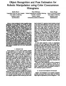
Figure 1: We propose a method for pose estimation in video sequences that finds the globally optimum pose trajectory given the single-frame pose distributions learned using regression. We create a graph where the nodes are sampled from single-image pose distributions (black circles). By finding the best pose path through the graph (marked by orange circles and arrows), we are able to recover from errors in the distribution as in frame t. Poses marked by a blue star are the result of taking the maximum mode of the single frame distribution.

1. Introduction Object pose estimation using category models has increasingly gained attention in the last decade, following the improvement of object recognition methods and the emerging interest in dealing with more complex scenarios. The orientation of generic objects, like beds or chairs, is exploited in scene understanding tasks for the correct labeling of scene items, as well as in robotic applications for grasp and control. While for some applications only a coarsely quantized pose value is enough, thus reducing the pose estimation problem to a simpler multi-view classification, for some others the output pose needs to be real-valued. This is the case of autonomous driving and augmented reality applications, where the object pose must be accurately estimated. Most of the approaches proposed in the literature address the pose estimation problem of object classes for still images [19, 3, 10, 11], while just a small number of

works have treated the same problem for videos. A natural strategy is to use a single-frame pose estimator and then combine the tentative estimations to obtain a final value for the pose in each frame, so that temporally incoherent results are filtered out or corrected. Some approaches rely on 3D-based pose estimators trained using CAD models and possibly deliver a real-valued pose [25, 18, 17, 27]. Since the availability of 3D models cannot be guaranteed, others have successfully explored the possibility of relying only on 2D data [20, 5]. Regardless of the pose estimator used, the combination in the temporal domain of singleframe results is in most cases obtained through suboptimal strategies, such as aggregation and fusion of pose estimation pdf’s over consecutive frames, or computationally ex1

pensive techniques, such as particle filtering.

1.1. Contributions We propose a method that combines a state-of-the-art 2D-based pose estimator [3], which provides a posterior probability distribution for the pose at each frame, with a linear programming formulation to exploit the temporal information and find the best pose trajectory for the entire video sequence. As our pose estimator exploits feature regression, we do not need to recur to 3D models to be able to provide a real-valued pose. Thanks to the usage of linear programming, we are able to handle inconsistencies in the output pose by estimating the globally optimal pose trajectory over the whole video sequence.

2. Related Works Pose estimation in single images While some works tackle the pose estimation problem as a classification problem by providing only a coarsely quantized value [19, 16, 7, 24], others have focused on delivering a continuous estimation for the pose. Among the latter, some exploit 3D information, either by training their algorithms with commercial CAD models [15] or by computing 3D sparse models using Structure-from-Motion techniques [26, 8]. Even if the usage of 3D models in pose estimation methods naturally leads to a real-valued pose, other approaches have been successful in delivering a continuous value by relying only on 2D models. In [9], the pose is refined by continuously deforming a view template after using a coarse view classifier, while [22] and [2, 3] apply feature regression on the whole set of object features or on each single patch, respectively. [11] learns a continuously pose-parametrized object model using structural SVM and then solves for the pose by finding the maximum in the inference problem. [10] trains a K-ary regression random forest by applying K-means at each splitting node on the basis of the training labels. Pose estimation in video sequences As labeled video datasets are increasingly made available [6, 25] and singleframe pose estimation approaches are now a mature tool to rely on, works have started to address the video-based pose estimation problem. In [18], a statistical manifold is learned from short video sequences of different class instances as a function of appearance and viewpoint, then a test video is divided in short sequences and a discrete pose is estimated by KL-divergence for each sequence. In [17], a statistical manifold is learned for spatio-temporal object parts, whose selection is driven by a twofold criterion of descriptiveness and distinctiveness, and then a discrete pose is estimated through KL-divergence. These works differ significantly from our method as they deliver only a very coarse viewpoint and no temporal information is actively employed. The works which are closest to our method are [20] and [25]. [20] relies on a modified Hough regression forest that

estimates the pose distribution at each frame, and then fuses it with a smoothed average of the past n distributions before determining the maximum a posteriori pose. This approach can be prone to error accumulation due to a sequence of wrongly estimated distributions. In contrast, our optimal formulation allows us to recover the correct pose even if the pose distribution is inaccurate for several consecutive frames. [25] estimates a probabilistic distribution at each frame combining the results of a pose estimator [24] and a motion prior on the viewpoint change. This work differs from ours in two aspects: (i) the pose estimator is based on parts learned from training images rendered from CAD models using a structural SVM optimization, while we only use 2D information; (ii) the maximum a posteriori pose is prone to error accumulation as it is obtained using a particle filtering framework that relies only on the past frame information, while we estimate the optimum pose over the whole sequence. Finally, a very different approach is presented in [5], where, within a traffic scene understanding framework, the pose estimation of vehicles is based upon the combination of vehicle tracklets, semantic scene labeling, scene flow and egomotion, and vanishing point estimation. Tracking The problem of pose estimation in video sequences can also be viewed as a tracking problem, where the goal is to find object pose trajectories in videos. Multiple object tracking has been commonly solved by expressing the problem as a linear program, either in monocular sequences [12] or multi-view sequences [13]. Human pose estimation can also benefit from the fusion of temporal information as shown in [21, 4], where both methods use dynamic programming to find the best pose trajectory for the video sequence.

3. Pose estimation of object classes In this section, we provide a description of the method by [3] that we leverage in our paper to obtain a posterior distribution for the object pose in each video frame. By using feature regression, we use only 2D information to derive the real-valued pose of the object.

3.1. Generative Feature Modeling At the very core of the method lie generative feature models, i.e., feature regressors that predict the appearance of each object patch as a function of the viewing angle. Feature regression relies on the smooth behavior of feature descriptor components when the corresponding patch undergoes a small change in viewpoint. Let ti = {(f1i , α1i ), (f2i , α2i ), . . . , (fni , αni )} be a feature track collecting the appearance of patch i under different viewpoints, i.e., a set of feature descriptors fji and corresponding viewpoint labels αji . For each feature track ti , we

define a generative feature model F i as F i (α) =

n X

G(α, αji )wji ,

(1)

j=1

i.e., a linear combination of Gaussian radial basis functions G centered at the training poses. Each basis function G(α, αji ) weighs the contribution of the vector coefficient wji according to the distance between the input pose α and the training pose αji . The vector coefficients wji are obtained as the solution of the following regularized linear least squares problem (Gi + λI)Wi = Zi ,

(2)

i where Gi is a n × n matrix such that Gilm = G(αli , αm ), i I is the identity matrix, W is the unknown coefficient matrix and Zi contains the feature descriptors arranged in row order. By collecting tracks stemming from a training sequence of a specific object, we can only predict the appearance of its patches. To move to a class level representation, we cluster all the training tracks of different instances on the basis of their similarity in descriptor and pose space using spectral clustering. As each cluster contains similar tracks, we can now predict a more general patch descriptor, thus accommodating for intra-class variations. The cluster regressor is based on a weighted linear combination of the responses of the individual regressors grouped in the cluster.

3.2. Estimation of the Pose Posterior Distribution Once we have learned a model as described above, we want to find correspondences between test and model features. After the matching step, we estimate the pose posterior distribution for each single frame as detailed in the following. Matching After extracting a set of features F = {f }M m=1 from the query frame, we need to establish matches between them and the class model, where the model is represented by a set C = {c}N 1 of feature cluster representatives. As our model includes no geometric information, we enforce feature-to-model correspondences to respect some loose geometric relation by using graph matching. Graph matching permits to disambiguate good and wrong matches at once on the basis of both feature descriptor distance and feature pairwise geometry. We interpret our test feature set and model feature set as the two graphs to be matched. Each test feature represents a node in the test graph G, while only a selection of the model features is used for the model graph G0 . In order to keep the problem tractable, we prune the model graph by considering only the K nearest neighbors for each test feature. K can

be a small value (K = 5 in our experiments) as we rely on the distinctiveness of gradient-based feature descriptors to directly prune wrong matches. The test graph is defined by G = (V, E, A), where V is the set of vertexes, E is the set of edges and A is the attribute matrix. A is defined such that ( fi for i = j Aij = , (3) αij for i 6= j where fi is the test descriptor, αij is the angle between the x-axis and the directed segment Pij connecting the two test feature locations. In [3], the off-diagonal entry is the pair (αij , rij ), where rij is the length of the segment Pij . By dropping this information, we make our matching approach scale-invariant. Therefore, we can handle a much larger range of object sizes, as is the case with images taken from real scenes. The model graph G0 is defined analogously, i.e., we consider the cluster representative as the model feature descriptor and the mean location of all the features in the cluster as its 2D location. Following our formulation, graph matching amounts to determine a mapping M = {(i, i0 )|i ∈ V, i0 ∈ V 0 } that maximizes the following score X S= g(Aij , A0i0 j 0 ), (4) (i,i0 )∈M,(j,j 0 )∈M

where g is a function that evaluates the similarity between two attributes. If we rewrite M as the binary vector x ∈ 0 {0, 1}nn , such that n = |V |, n0 = |V 0 |, and xii0 = 1 if (i, i0 ) ∈ M , the solution is x∗ = arg max S = arg max xT Wx, x

x nn0

s.t . x ∈ {0, 1}

(5)

and kxk2 = n,

where W is a nn0 × nn0 matrix such that Wii0 ,jj 0 = g(Aij , A0i0 j 0 ) and is defined as

Wii0 ,jj 0

 log(m − dii0 + 1)     2   m 1 − τβ1 =      0

if i = j and i0 = j 0 if β ≤ τ1 and

(i 6= j or i0 6= j 0 ) otherwise

(6)

For individual matches, g evaluates the descriptor distance. Since dii0 = kfi − fi0 k is the Euclidean distance in descriptor space and m = max dii0 , a high diagonal entry reflects a plausible individual match. For pairwise matches, g evaluates the geometric consistency of the feature locations. Since β = |αij − αi0 j 0 | is the angular distance, a high offdiagonal entry reflects a pair of matching features that are consistent in their respective orientation. In Eq. 5, we fix the norm of the solution so that each test feature is matched to a

model feature, although the assignment may not be one-toone. We are not concerned about this, as wrong assignments will be penalized in the graph matching result. Since Integer Quadratic problems are NP-hard, we decide for an approximate solution through linear relaxation, following [14]. For arbitrary fixed norm, the maximization problem is equivalent to x∗ = arg max S = arg max x

s.t . x ∈ [0, 1]

x nn0

xT Wx xT x

m

(7)

2

and kxk = n.

This expression is a classical √ Rayleigh quotient problem nvmax , where vmax is the whose solution is x∗ = dominant eigenvector of W . Since the linear relaxation has changed the matching constraint from many-to-one to many-to-many, now only the relative amplitude of the solution components is relevant. Therefore, we can enforce the solution to have unit norm without loss of generality, so that x∗ = vmax and |x∗ii0 | ≤ 1. Since W has only non-negative entries, the Perron-Frobenius’ theorem guarantees that x∗ii0 ≥ 0. Therefore, we fully meet the constraint 0 x ∈ [0, 1]nn and, as a byproduct, we can directly interpret the solution in probabilistic terms. Pose Estimation Since we are interested in estimating the pose distribution, we interpret the pose estimation problem in a probabilistic fashion. More specifically, we define a probability p(α, c|f ) for each test feature f that expresses the likelihood of observing f from viewpoint α and that c is a correct match for f . By applying the probability chain rule, we obtain p(α, c|f ) = p(α|f, c)p(c|f ).

We extend our reasoning from one query feature to all query features F = {f }M m=1 by assuming a mixture model where each feature contributes equally in order to avoid cancellation problems. Therefore, the posterior distribution for the pose is X p(α, c|F) ≈ p(α|fm , c)p(c|fm ) (11)

(8)

The first factor p(α|f, c) is defined in terms of the generative feature model as   X ui (ei )T (Ri )−1 ei exp − G(α, βi ), p(α|f, c) = U 2 i:ti ∈c (9) where ui weighs the contribution of the i-th regressor and U is a normalization constant; e = f − F i (α) is the prediction error made by the i-th regressor in cluster c with respect to f ; Ri is the covariance matrix of the i-th regressor estimated during training; βi = arg minj |α − αji | weighs the view consistency of the i-th regressor in cluster c to the tentative pose α. In a nutshell, a high value will result if the regressor prediction agrees with the query feature at the tentative pose α and α is consistent with the regressor training views. We derive the term p(c|f ) in a straightforward manner from the matching step. Since kx∗ k2 = 1 and x∗f c ∈ [0, 1], we can express our confidence about the correctness of the match as p(c|f ) = (x∗f c )2 . (10)

Once we have this distribution for each frame of the video sequence, our goal is to find the most consistent set of poses over all frames. We do this in a globally optimum way by constructing a graph, where each node consists of a pose sampled from the distribution of Eq. (11). The goal is to find the best path in the graph, which we do by solving a linear problem, as explained in the next section.

4. Temporal pose estimation In this section, we present how to solve the pose estimation problem in video sequences by taking into account the evidence of all the frames, as computed in the previous section, to find a globally optimal pose trajectory. Let O = {otk } be a set of pose observations with t ok = (αkt , stk ), where αkt is the estimated pose and stk is the score or probability of that pose in that frame obtained from the distribution of Eq. (11). A path is defined as a list of ordered pose observations T = {otk11 , otk22 , · · · , otkNN } with t1 ≤ t2 ≤ . . . ≤ tN and our goal is to find the path T ∗ that best explains the pose observations. This is equivalent to finding the T that maximizes the posterior probability given the set of pose observations O, which is known as the maximum a posteriori or MAP problem. T ∗ = arg max P (T |O)

(12)

T

By further assuming that the observations are conditionally independent, the equation can be rewritten as: T ∗ = arg max P (O|T )P (T ) T Y = arg max P (ok |T )P (T ), T

(13) (14)

k

where P (ok |T ) corresponds to the score of the pose sk according to the learned pose distribution, and P (T ) can be represented by a Markov chain: N P (T ) = Pin (o1k1 ) . . . P (otkt |ot−1 kt−1 ) . . . Pout (okN ).

(15)

4.1. Mapping to a linear program This formulation can be directly mapped into a minimum cost network flow problem. We define a directed graph

u1

u3

v3

u4

v4

v1

s

u5

v6

u7

v7

t

v2

u2

u6

v5

Figure 2: Example of a graph spanning 3 frames, with the special source s and sink t nodes, and a total of 7 pose observations represented by two nodes each: beginning ui and end vi nodes. The optimal path is marked by orange arrows. G = (V, E) with costs C(i, j) and capacities u(i, j) associated with every edge (i, j) ∈ E. An example of such a network is shown in Figure 2; it contains two special nodes, the source s and the sink t; all flow that goes through the graph starts at the s node and ends at the t node. Our goal is to find the best path through the network, i.e., the path with minimum cost. Each pose observation oi is represented with two nodes, the beginning node ui ∈ V and the end node vi ∈ V (see Figure 2). A score edge connects ui and vi . Finding the best path can be expressed as a Linear Program which is defined by a linear objective function and a set of linear constraints. Linearization of the objective function of Eq. (14) is obtained by defining a set of flow flags f (i, j) = {0, 1} which indicate if an edge (i, j) is part of the optimum path solution or not. By defining the costs as negative log-likelihoods and combining Eqs. (14) and (15), the following objective function is obtained: X T ∗ = arg min − log P (T ) − log P (ok ) T

k

= arg min f

+

X

X

Cin (i)fin (i) +

i

X

Ct (i, j)ft (i, j)

i,j

Csc (i)fsc (i) +

i

X

Cout (i)fout (i)

(16)

i

subject to the constraint that the flow that enters a node is equal to the flow that leaves the node: P fin (i) + ft (j, i) = fsc (i) j

fsc (i) + fout (i) =

X

edges connecting a pose observation from frame t to frame t + n. This cost represents the pose difference between the two observations. Assuming that an object’s pose does not change a lot from one frame to the next, we define these costs to be an increasing function of the distance between pose observations. Therefore, the cost of a link edge is defined as:   kαt −αt k (18) Ct (i, j) = − log 1 − jMα i + C(∆f )   ∆f −1 where C(∆f ) = − log Bjump is the cost depending on the frame difference between pose observations. For all our experiments we allow matches up to two frames apart, which allows us to recover from pose estimation errors that occur on isolated frames. We set the parameter Bjump = 0.3. Edges between observations are only created if their pose distance is less than Mα degrees apart. This parameters allows us to adapt the algorithm to different frame rates and object speeds. The score costs Csc (i) correspond to the pose observations and express how probable is that particular pose according to the learned distribution of Eq. (11). The cost is defined as:  t  si Cdet (i) = log , (19) Ms where Ms is a normalization factor equivalent to the maximum score of all pose observations. The entrance cost Cin (i) and exit cost Cout (i), are set to 0 in our case, since we do not penalize any of the initial or last pose observations. The solution can be found efficiently using any solver like Simplex or shortest path [1].

5. Experimental Results In this section, we first show results on a toy example from the EPFL multi-view car dataset [19]. Later, we test the proposed algorithm on two real-world sequences, namely KITTI [6] and Youtube [25] and show the superior performance of our method.

5.1. Toy example - EPFL Dataset ft (i, j).

(17)

j

Furthermore, we know that f (i, j) = {0, 1}, a condition that we relax into 0 ≤ f (i, j) ≤ 1. This tight relaxation allows us to have a linear program without losing the optimality guarantee. Finally, the overall flow that leaves s has to be 1, as well as the flow that enters t. As we can see in Eq. (16), there are four types of costs corresponding to four types of edges as shown in Figure 2. The link or transition costs Ct (i, j) corresponding to the link

This dataset consists of twenty sequences of cars rotating on a platform. Since the shooting time is given, it is possible to compute a precise orientation of the object in each frame. We consider this as a toy example on which to test our method because cars have a high variability in appearance but the change in orientation is smooth and predictable. We compare our method to six single-frame state-of-theart pose estimators [3, 2, 11, 10, 22, 19] and one videobased approach that has been recently proposed [20]. We

Method

MAE [◦ ] 90th perc.

MAE [◦ ] 95th perc.

MAE [◦ ]

19.4 14.51 7.73 12.67 3.91

26.7 22.83 16.18 17.77 4.30

46.48 33.98 31.27 29.7 24.24 23.38 15.8 4.89

23.13 14.41 15.53 5.6

26.85 22.72 19.27 6.26

34.90 31.16 24.53 7.10

50% split Ozuysal et al. [19] Torki et al. [22] Fenzi et al. [2] R.-C. et al. [20] Hara et al. [10] Fenzi et al. [3] He et al. [11] Proposed Leave-One-Out split Torki et al. [22] Fenzi et al. [2] Fenzi et al. [3] Proposed

Table 1: EPFL dataset. Mean Absolute Error (MAE) and its 90th and 95th percentiles. The two leftmost columns show a clearer insight into the algorithms performance by removing the influence of large errors from the overall mean. used the same testing framework as previous works, i.e., two different splits for training and testing. (i) 50% Split: training the model on the first 10 sequences and testing it on the remaining 10; (ii) Leave-One-Out: training the model on 19 sequences and testing it on the remaining one. We build our model according to Section 3 and we estimate the pose posterior distribution in each frame as explained in Section 3.2. For each frame, we extract N = 10 equally spaced pose values from the posterior distribution and construct the graph over all frames of the sequence. The best path is found using the Gurobi Library [23]. In Table 1, we show that our method not only outperforms all the other single-frame pose estimators, but it also obtains more accurate results than the other video-based approach [20]. In particular, our Mean Absolut Error (MAE) is approximately 80% smaller with respect to the results published in [11], which is the most accurate method on this dataset so far. As the results in the first two columns show, the overall mean is strongly affected by few yet detrimental 180◦ flipping errors. As our method does not take hard decisions in each frame but finds the path of orientations that best explains the whole sequence, we can reduce the effect of these wrong estimations to a minimum.

5.2. Youtube and KITTI datasets In order to test the performance of our method in realworld scenarios, we evaluate it on two datasets which emphasize the topological appearance changes of the target. The first test set consists of 11 sequences from the KITTI benchmark dataset [6], which were annotated by [25]. They

show real-world scenarios of busy streets, where target cars undergo significant viewpoint changes. In some sequences, the car is partially or even totally occluded by other cars or pedestrians, making the pose estimation problem very challenging. An important difficulty of this dataset is that the car size varies significantly during each sequence, ranging from 500 pixels down to 40 pixels, as a result of the relative motion between the moving camera and the car. We followed the same paradigm as in the toy example. We extract features from each test image, we matched them against the model, which is learned from the first 10 sequences of the EPFL dataset, and then we obtain a pose posterior distribution. Finally, we sample N equally spaced values from the posterior distribution, we construct the graph over all frames, and we find the path that best explains the sequence. To cope with the small size of the targets, we upsample the images by 2, since our approach is based on local sparse features and we need a minimum amount of features to estimate a reliable posterior distribution. In order to evaluate viewpoint estimation, we report two metrics: (i) viewpoint accuracy, where the estimated viewpoint is considered correct if the deviation from the ground truth viewpoint is less than 15◦ ; (ii) mean absolute error, which reports the mean absolute difference in degrees between the estimated and the ground truth viewpoints for the entire sequence. As we only tackle the pose estimation problem, we use the ground truth bounding boxes as input to our algorithm. In Table 2, we compare our results on each KITTI sequence and the overall mean with [25]. The notation “1. GT” indicates that the ground truth orientation of the first frame is used to initialize the method. Not only our method outperforms [25] reducing the error by approximately 40% and increasing accuracy by 20 percentage points when the ground truth of the first frame is used, but we also obtain better results when this advantage is not used. As a further insight into our algorithm we provide two frame-by-frame graphs from the KITTI dataset, where we plot the results of the single-frame pose estimator, the pose value selected by the LP tracker, and the ground truth. In the first graph, the LP tracker is able to completely recover from the spurious errors of the single-frame pose estimator, as a correct evidence is provided in most frames. However, when correct evidence is more counterbalanced by opposite, wrong evidence, as in the second plot around frame 23, the LP tracker adopts a conservative solution and just outputs the pose in the middle. Additionally, we provide a visual example of our algorithm in Fig. 4, where we estimate the pose of the car pointed by the red arrow. The pose estimation is accurate even when the car is fully occluded. We also perform experiments on the Youtube dataset [25], which contains 9 sequences where a racing car under-

Proposed 1. GT

Proposed

Xiang et al. 1.GT [25]

Xiang et al. [24]

Fenzi et al. [3]

KITTI01 KITTI02 KITTI03 KITTI04 KITTI05 KITTI06 KITTI07 KITTI08 KITTI09 KITTI10 KITTI11

1.00/4.04◦ 0.81/9.74◦ 0.81/9.75◦ 0.72/10.55◦ 0.93/4.35◦ 1.00/5.02◦ 0.78/12.78◦ 0.70/10.74◦ 0.90/8.23◦ 0.92/7.09◦ 0.54/16.00◦

0.96/5.54◦ 0.67/12.81◦ 0.46/16.33◦ 0.65/12.10◦ 0.93/5.93◦ 1.00/5.08◦ 0.21/24.8◦ 0.81/10.00◦ 0.90/8.33◦ 0.92/7.18◦ 0.48/29.7◦

0.95/6.5◦ 1.00/5.40◦ 0.42/15.64◦ 0.22/27.05◦ 0.36/23.59◦ 0.31/21.63◦ 0.96/6.86◦ 0.57/15.61◦ 0.50/21.63◦ 0.81/7.99◦ 0.88/9.33◦

0.57/44.46◦ 0.33/119.54◦ 0.50/15.99◦ 0.17/58.42◦ 0.64/23.65◦ 0.59/20.29◦ 0.70/24.50◦ 0.67/23.26◦ 0.50/17.60◦ 0.44/56.78◦ 0.68/12.29◦

0.35/64.87◦ 0.22/72.45◦ 0.13/62.81◦ 0.24/63.11◦ 0.76/12.82◦ 0.71/12.72◦ 0.09/56.80◦ 0.52/42.00◦ 0.33/32.85◦ 0.47/49.20◦ 0.32/76.17◦

Mean

0.83/8.93◦

0.73/12.53◦

0.63/14.66◦

0.53/37.89◦

0.38/49.62◦

Table 2: KITTI dataset. Viewpoint accuracy/mean absolute error (MAE) in degrees 300

250

Groundtruth LP Single−frame

75°

59°

Pose

200

150

100

50

0 0

5

10

15

20 25 30 Frame number

35

40

45

69°

61°

50

350 Groundtruth LP Single−frame

300

34°

31°

Pose

250 200

Figure 4: Visual results of our algorithm when estimating the pose of the car pointed by the red arrow. Ground truth in red, algorithm estimation in green.

150 100 50 0 0

5

10

15 Frame number

20

25

30

Figure 3: Ground truth pose (red), pose output by choosing the highest mode of the pose distribution (blue), optimal solution provided by the proposed method (green).

goes significant orientation changes. In many sequences, pictures are very blurred as a result of the high speed, and often the car is surrounded by smoke, due to the sliding of tires on the ground, making the pose estimation problem extremely challenging. As we can see, we outperform [25] also on this dataset. Interestingly, we observe that the two methods are complementary. As we can see in sequences SUV2, KITTI04-06, [25] performs poorly while our method is able to achieve very high viewpoint accu-

racy. On the contrary, in sequences KITTI11 or Race3, [25] outperforms our method. This could lead to a potentially interesting line of work in which both methods could be combined for an even better performance.

6. Conclusions In order to solve the pose estimation problem for object categories in videos, we proposed a method that embeds the results of a single-frame pose estimator in a linear programming formulation. We create a pose graph by sampling values from the posterior probability distributions delivered at each frame and we find the pose trajectory that best explains the entire video sequence. Unlike previous approaches that suffer from error accumulation in case of wrongly estimated distributions, our optimal formulation allows us to recover the correct orientation even if distributions are inaccurate

Proposed 1. GT

Proposed

Xiang et al. 1. GT [25]

Xiang et al. [24]

Fenzi et al. [3]

Race1 Race2 Race3 Race4 Race5 Race6 SUV1 SUV2 Sedan

0.58/16.64◦ 0.80/9.51◦ 0.55/16.20◦ 0.69/10.87◦ 0.73/11.39◦ 0.68/15.54◦ 0.94/4.88◦ 0.89/6.42◦ 0.72/12.20◦

0.54/18.47◦ 0.74/10.35◦ 0.55/16.29◦ 0.56/17.85◦ 0.55/18.01◦ 0.47/16.93◦ 0.93/5.29◦ 0.61/15.14◦ 0.71/12.32◦

0.67/18.73◦ 0.77/10.83◦ 0.83/9.28◦ 0.69/15.83◦ 0.71/10.75◦ 0.43/18.47◦ 0.82/7.81◦ 0.57/19.56◦ 0.76/9.87◦

0.52/42.62◦ 0.53/44.30◦ 0.64/46.08◦ 0.79/13.37◦ 0.54/57.79◦ 0.31/37.08◦ 0.47/78.38◦ 0.39/63.41◦ 0.79/20.84◦

0.09/79.88◦ 0.36/54.26◦ 0.22/66.63◦ 0.20/62.47◦ 0.23/45.92◦ 0.43/44.90◦ 0.14/78.65◦ 0.44/36.07◦ 0.40/23.05◦

Mean

0.71/12.18◦

0.63/13.86◦

0.69/13.46◦

0.54/47.24◦

0.28/54.67◦

Table 3: Youtube dataset. Viewpoint accuracy/mean absolute error (MAE) in degrees. for several consecutive frames. Experiments on two challenging datasets encompassing urban scenes and car races show that our approach significantly outperforms state-ofthe-art algorithms.

References [1] R. Ahuja, T. Magnanti, and J. Orlin. Network flows: Theory, algorithms and applications. Prentice Hall, Upper Saddle River, NJ, USA, 1993. [2] M. Fenzi, L. Leal-Taix´e, B. Rosenhahn, and J. Ostermann. Class Generative Models based on Feature Regression for Pose Estimation of Object Categories. In CVPR, 2013. [3] M. Fenzi and J. Ostermann. Embedding Geometry in Generative Models for Pose Estimation of Object Categories. In BMVC, 2014. [4] M. Fergie and A. Galata. Dynamical pose filtering for mixtures of gaussian processes. BMVC, 2007. [5] A. Geiger, M. Lauer, C. Wojek, C. Stiller, and R. Urtasun. 3d traffic scene understanding from movable platforms. TPAMI, 2014. [6] A. Geiger, P. Lenz, and R. Urtasun. Are We Ready for Autonomous Driving? The KITTI Vision Benchmark Suite. In CVPR, 2012. [7] A. Ghodrati, M. Pedersoli, and T. Tuytelaars. Is 2D Information Enough For Viewpoint Estimation? In ECCV, 2014. [8] D. Glasner, M. Galun, S. Alpert, R. Basri, and G. Shakhnarovich. Viewpoint-Aware Object Detection and Pose Estimation. In ICCV, 2011. [9] C. Gu and X. Ren. Discriminative Mixture-of-templates for Viewpoint Classification. In ECCV, 2010. [10] K. Hara and R. Chellappa. Growing Regression Forests by Classification: Applications to Object Pose Estimation. In ECCV, 2014. [11] K. He, L. Sigal, and S. Sclaroff. Parameterizing object detectors in the continuous pose space. In ECCV, 2014. [12] L. Leal-Taix´e, M. Fenzi, A. Kuznetsova, B. Rosenhahn, and S. Savarese. Learning an Image-based Motion Context for Multiple People Tracking. In CVPR, 2014. [13] L. Leal-Taix´e, G. Pons-Moll, and B. Rosenhahn. Branchand-price global optimization for multi-view multi-target tracking. CVPR, 2012.

[14] M. Leordeanu and M. Hebert. A Spectral Technique for Correspondence Problems Using Pairwise Constraints. In ICCV, 2005. [15] J. Liebelt and C. Schmid. Multi-View Object Class Detection with a 3D Geometric Model. In CVPR, 2010. [16] R. J. L´opez-Sastre, T. Tuytelaars, and S. Savarese. Deformable Part Models Revisited: A Performance Evaluation for Object Category Pose Estimation. In ICCV Workshops, 2011. [17] L. Mei, J. Liu, A. O. Hero, and S. Savarese. Robust Object Pose Estimation via Statistical Manifold Modeling. In ICCV, 2011. [18] L. Mei, M. Sun, K. Carter, A. Hero, and S. Savarese. Unsupervised object pose classification from short video sequences. In BMVC, 2009. ¨ [19] M. Ozuysal, V. Lepetit, and P. Fua. Pose Estimation for Category Specific Multiview Object Localization. In CVPR, 2009. [20] C. Redondo-Cabrera, R. L´opez-Sastre, and T. Tuytelaars. All together now: Simultaneous object detection and continuous pose estimation using a hough forest with probabilistic locally enhanced voting. In BMVC, 2014. [21] C. Sminchisescu and A. Jepson. Variational mixture smoothing for non-linear dynamical systems. CVPR, 2004. [22] M. Torki and A. M. Elgammal. Regression from Local Features for Viewpoint and Pose Estimation. In ICCV, 2011. [23] www.gurobi.com. Gurobi library. [24] Y. Xiang and S. Savarese. Estimating the Aspect Layout of Object Categories. In CVPR, 2012. [25] Y. Xiang, C. Song, R. Mottaghi, and S. Savarese. Monocular Multiview Object Tracking with 3D Aspect Parts. In ECCV, 2014. [26] J. Xiao, J. Chen, D.-Y. Yeung, and L. Quan. Structuring Visual Words in 3D for Arbitrary-View Object Localization. In ECCV, 2008. [27] M. Zeeshan Zia, M. Stark, and K. Schindler. Explicit Occlusion Modeling for 3D Object Class Representations. In CVPR, 2013.