Dec 2, 2014 - lossy media to show that also local field temperatures exhibit oscillations ..... rate in the vicinity of a lossy material layer with refractive index nc ...
Position-dependent photon operators in the quantization of the electromagnetic field in dielectrics at local thermal equilibrium Mikko Partanen, Teppo H¨ayrynen, Jani Oksanen, and Jukka Tulkki Department of Biomedical Engineering and Computational Science, Aalto University, P.O. Box 12200, 00076 Aalto, Finland
arXiv:1412.0796v1 [quant-ph] 2 Dec 2014
ABSTRACT It has very recently been suggested that asymmetric coupling of electromagnetic fields to thermal reservoirs under nonequilibrium conditions can produce unexpected oscillatory behavior in the local photon statistics in layered structures. Better understanding of the predicted phenomena could enable useful applications related to thermometry, noise filtering, and enhancing optical interactions. In this work we briefly review the field quantization and study the local steady state temperature distributions in optical cavities formed of lossless and lossy media to show that also local field temperatures exhibit oscillations that depend on position as well as the photon energy. Keywords: quantum optics, field quantization, ladder operators, photon number
1. INTRODUCTION The quantum optical processes and quantization of the electromagnetic (EM) field in lossy structures exhibiting interference have been widely studied during the last few decades especially in layered structures.1–6 Describing the spatial evolution even in the most relevant quantum approaches based on the input-output relation formalism (IORF) of the photon creation and annihilation operators and direct quantization of Maxwell’s equations has been incomplete in the sense that they do not provide a unique way to determine photon number. This is reflected by the observation that the vector potential and electric field operators obtained by using the IORF obey the well-known canonical commutation relation for an arbitrary choice of normal mode functions as expected,4, 5 but the commutation relations of the ladder operators do not. The anomalous commutation relations of the ladder operators were studied in several reports7–11 but no clear resolution for the anomalies was found apart from reaching a consensus that the anomalies were irrelevant as long as the field commutation relations and classical field quantities were well defined. Since then, the IORF has mainly been applied in calculating the classical field quantities until the very recent suggestions that, despite the early interpretations, the ladder operators and their commutation relations might in fact relate to measurable physical properties12 and finding well derived operators can significantly simplify the description of energy transfer.13 We have recently introduced photon ladder operators associated with the vector potential in a way that is consistent with the canonical commutation relations and gives further insight on the local effective photon number, thermal balance, and the formation of the local thermal equilibrium.13 One interesting result is that the field at each point in a vacuum cavity couples differently to the surrounding material layers suggesting a position-dependent local photon number and temperature. The position dependence is expected to be directly observable using experimental setups in which the field-matter interaction is dominated by the coupling to the electric field. In this paper, we apply our quantum fluctuational electrodynamics approach to describe the EM field in lossless and lossy cavity geometries. We start by a short review of the theoretical background to the EM field quantization, photon operators, and their relation to thermal balance. This is followed by applying the presented theoretical concepts to study the position and photon energy dependence of the effective field temperature, electrical contribution of the local density of EM states, Poynting vector, and net emission rate in two cavity geometries: a vacuum cavity formed between two semi-infinite thermal reservoir media at different temperatures, and a similar structure where the cavity medium is lossy.
2. FIELD QUANTIZATION For completeness of the theoretical foundations of the present work, we first give an overview of the results originally presented by Matloob et al.5 to lay the ground for our recently defined ladder and photon-number operators.13 After that the ladder and photon-number operators are presented and their relation to the Poynting vector and thermal balance is discussed.
2.1 Overview of the noise operator formalism for EM field quantization The electromagnetic waves are considered to propagate parallel to the x axis with their transverse electric and ˆ t) and B(x, ˆ t) parallel to the y and z axes, respectively. The field operators are magnetic field operators E(x, ˆ t) by the relations5 related to the vector potential operator A(x, ˆ + (x, ω) = iω Aˆ+ (x, ω), E ˆ + (x, ω) = ∂ Aˆ+ (x, ω) B ∂x
(1) (2)
ˆ − (x, ω), B ˆ − (x, ω), and Aˆ− (x, ω) are Hermitian conjugates for positive frequencies. The negative frequency parts E of the positive frequency parts. The field operators satisfy the frequency domain Maxwell’s equations and, when the relations in Eqs. (1) and (2) are used, the vector potential operator can be shown to satisfy the one-dimensional nonhomogeneous Helmholtz equation5 ∂ 2 ˆ+ ω 2 n(x, ω)2 ˆ+ A (x, ω) + A (x, ω) = −µ0 Jˆem (x, ω), (3) ∂x2 c2 where µ0 is the permeability of vacuum, n(x, ω) is the refractive index of the medium, and Jˆem (x, ω) = j0 (x, ω)fˆ(x, ω) is a Langevin noise current operator presented in terms of the scaling factor j0 (x, ω) and the modified Langevin force operator fˆ(x, ω) which is a bosonic field operator defined through the following commu0 tation relations [fˆ(x, ω), fˆ† (x0 , ω 0 )] = δ(x − x0 )δ(ω − ω 0 ) and [fˆ(x, ω), fˆ(x0 , ω p )] = [fˆ† (x, ω), fˆ† (x0 , ω 0 )] = 0. The scaling factor of the Langevin noise current operator is given by j0 (x, ω) = 4π~ω 2 ε0 Im[n(x, ω)2 ]/S, where ~ is the reduced Planck’s constant, ε0 is the permittivity of vacuum, and S is the area of quantization in the y-z plane.5 The quantization area only affects the scaling of the field quantities and in the calculations we set S = 1 m2 . The magnitude of the scaling factor has been determined by requiring that the vector potential and electric field operators obey the canonical equal-time commutation relation as detailed in Ref.5 . The solution to Eq. (3) can be written in terms of the Green’s function of the Helmholtz equation as Z ∞ + ˆ A (x, ω) = µ0 j0 (x0 , ω)G(x, ω, x0 )fˆ(x0 , ω)dx0 .
(4)
−∞
The Green’s function depends on the problem geometry via the refractive index of the medium. The Green’s function for the studied two interface geometry is given in Ref.13 . In order to write the field operators in compact forms, we define the scaled forms of the Green’s functions: GA (x, ω, x0 ) =µ0 j0 (x0 , ω)G(x, ω, x0 ),
(5)
GE (x, ω, x0 ) =iµ0 ωj0 (x0 , ω)G(x, ω, x0 ),
(6)
GB (x, ω, x0 ) =
iµ0 ωn(x, ω) j0 (x0 , ω)[GR (x, ω, x0 ) − GL (x, ω, x0 )], c
(7)
where GE (x, ω, x0 ) and GB (x, ω, x0 ) are obtained from GA (x, ω, x0 ) by using Eqs. (1) and (2), and GR (x, ω, x0 ) and GL (x, ω, x0 ) are the right and left propagating parts of the Green’s function identified from the factors eikx and e−ikx , respectively. In this paper, when treating lossless semi-infinite media, an infinitesimal imaginary part of the refractive index is assumed in j0 (x, ω) and G(x, ω, x0 ) and it is set to zero after calculating the integrals. R∞ Using the above definitions the vector potential operator is given by Aˆ+ (x, ω) = −∞ GA (x, ω, x0 )fˆ(x0 , ω)dx0
ˆ + (x, ω) and B ˆ + (x, ω). In time domain the fields are given by the and corresponding expressions are valid for E R ˆ t) = 1 ∞ Aˆ+ (x, ω)e−iωt dω + H.c., where inverse Fourier transforms of the frequency domain operators as A(x, 2π 0 ˆ t) and B(x, ˆ t) are obtained from similar the Hermitian conjugate is the negative frequency part. Again, E(x, expressions. ˆ ˆ The electric displacement field operator D(x, t) and the magnetic field strength operator H(x, t), needed, e.g., in calculating the Poynting vector, are obtained from the electric field and magnetic field density operators ˆ + (x, ω) = ε0 ε(x, ω)E ˆ + (x, ω) and B ˆ + (x, ω) = µ0 µ(x, ω)H ˆ + (x, ω), where ε(x, ω) using the constitutive relations D and µ(x, ω) are the position-dependent relative permittivity and permeability of the medium.14
2.2 Ladder and photon-number operators In any quantum electrodynamics (QED) description, the canonical commutation relations are satisfied for field ˆ t), E(x ˆ 0 , t)] = −i~/(ε0 S)δ(x − x0 ),15 but the same is not generally true for the canonical quantities, i.e., [A(x, commutation relations of the ladder operators. The dominant approach in evaluating the ladder operators has been to separate the field operators obtained from QED either into the left and right propagating normal modes or into the normal modes related to the left and right inputs and the corresponding ladder operators so that the vector potential can be written as Aˆ+ (x, ω) = uR (x)ˆ aR (ω) + uL (x)ˆ aL (ω).8, 10, 16 This is tempting in view of the analogy with classical EM, but in most cases results in ladder operators that are not unambiguously determined due to the possibility to scale the normal modes nearly arbitrarily. Also divisions accounting for the noise contribution and more physically transparent interpretations11 have been reported, but they do not give the canonical commutation relations for the ladder operators either. We have adopted a different starting point to preserve the canonical commutation relation [ˆ a(x, ω), a ˆ† (x, ω 0 )] = 0 δ(ω − ω ) by defining the photon annihilation operator to be proportional to the total vector potential operator and normalizing it so that the commutation relation is fulfilled.13 Our approach gives the photon annihilation operator as r ε0 ω a ˆ(x, ω) = Aˆ+ (x, ω), (8) 2π 2 ~ρ(x, ω) where we have used the conventional definition for the electrical contribution of the local density of EM states (electric LDOS) as17 2ω ρ(x, ω) = 2 Im[G(x, ω, x)]. (9) πc S R † The photon-number operator is given in terms of the ladder operators as n ˆ (x, ω) = a ˆ (x, ω)ˆ a(x, ω 0 )dω 0 and its expectation value is expressed in terms of the Green’s function as Z ∞ ε0 ω |GA (x, ω, x0 )|2 hˆ η (x0 , ω)idx0 . (10) hˆ n(x, ω)i = 2π 2 ~ρ(x, ω) −∞ R Here we have defined a source field photon-number operator as ηˆ(x, ω) = fˆ† (x, ω)fˆ(x0 , ω 0 ) dx0 dω 0 and assumed that the noise operators at different positions and at different frequencies are uncorrelated so that the source field photon-number expectation value at position x of a thermally excited medium is hˆ η (x, ω)i =
1 , e~ω/(kB T (x)) − 1
(11)
where kB is the Boltzmann constant and T (x) is the position-dependent temperature of the medium. In the case of thermal fields the photon-number operator in Eq. (10) also allows one to calculate an effective local field temperature for the electric field as T (x, ω) =
~ω . kB ln[1 + 1/hˆ n(x, ω)i]
(12)
In the above definition, the ladder operators are essentially defined to be proportional to the total vector potential (and therefore also the electric field) operator including the contribution from all the source points.
Furthermore, the photon-number operator can be considered as an effective operator that partly reflects the physical properties of the electric field. For instance, under certain nonequilibrium conditions studied in Sec. 3, the photon number can oscillate due to the interference seen in the electric fields. It is also found that without the above exact form for the position-dependent normalization coefficient the resulting photon-number expectation value oscillates near material interfaces at thermal equilibrium. The properly normalized annihilation operator defined in Eq. (8) always results in a photon-number expectation value that is constant everywhere at thermal equilibrium.
2.3 Poynting vector and thermal balance For additional physical insight, we will compare the position dependence of the photon-number expectation value following from Eq. (10) to the well-known energy flux given by the Poynting vector. The expectation value of the one-dimensional quantum optical Poynting vector operator is given in terms of the electric and magnetic field Green’s functions and the source field photon-number expectation value as13 Z 1 ˆ Re[G∗E (x, ω, x0 )GH (x, ω, x0 )]hˆ η (x0 , ω)idx0 , (13) hS(x, t)iω = 2π 2 where GH (x, ω, x0 ) = GB (x, ω, x0 )/(µ0 µ(x, ω)). The brackets denote the expectation value over all states resulting in the source field photon-number expectation value of Eq. (11), and the subscript ω denotes the spectral component of the Poynting vector, i.e., the integrand when the total Poynting vector is expressed as an integral over positive frequencies. For a better understanding of the introduced photon-number concept it is essential to consider its contribution to local energy balance at position x. The Poynting theorem relates the local power dissipation and generation to the current density and electric field at position x and to the divergence of the Poynting vector.18 Therefore, in one dimension, the spectral energy transfer rate hQ(x, t)iω , i.e., the spectral net emission between the field and the medium at position x, is given by ∂ ˆ ˆ t)E(x, ˆ t)iω . hS(x, t)iω = −hJ(x, (14) ∂x ˆ t) = Jˆabs (x, t) − Jˆem (x, t) consists of parts corresponding to absorption and emisThe current density term J(x, sion. The photon emission is described by the Langevin noise current operator Jˆem (x, ω) = j0 (x, ω)fˆ(x, ω) introˆ + (x, ω) duced as a field source in Eq. (3). The photon absorption term is of the form Jˆabs (x, ω) = ε0 ω Im[n(x, ω)2 ]E so that the absorption rate is proportional to the square of the electric field, or equivalently the electric field fluctuation. Substituting the time domain current terms (i.e., the Fourier transforms of the frequency domain terms) to Eq. (14) and calculating the expectation values over source field photon-number states gives the local net emission rate in terms of the photon numbers of the source and the total electromagnetic fields as hQ(x, t)iω =
hQ(x, t)iω = ~ω 2 Im[n(x, ω)2 ]ρ(x, ω)[hˆ η (x, ω)i − hˆ n(x, ω)i].
(15)
Equation (15) directly shows that the local net emission rate is zero only if the material is lossless (Im[n(x, ω)2 ] = 0), the electric LDOS is zero [ρ(x, ω) = 0], or the field is at local thermal equilibrium [hˆ n(x, ω)i = hˆ η (x, ω)i]. Equation (15) also nicely separates the effect of temperature and wave features in the local net emission rate: the effect of temperature is described by the photon-number operators and the effect of wave features is described by the imaginary part of the Green’s function. In resonant systems where the energy exchange is dominated by ˆ ω)iω = 0 can be used to approximately determine the steady state a narrow frequency band, condition hQ(x, temperature of a weakly interacting resonant particle.19 This leads to concluding that in order to reach a thermal balance with the field, the particle must reach a temperature that is equal to the effective field temperature so that the term hˆ η (x, ω)i − hˆ n(x, ω)i disappears.
3. RESULTS To investigate the physical implications of the concepts presented in Sec. 2 we study the electric LDOS, effective field temperature, Poynting vector, and net emission rate in two geometries: a vacuum cavity formed between two semi-infinite thermal reservoir media at different temperatures, and a similar structure where the cavity medium is lossy.
(a)
(b)
Electric LDOS (2/(πcS))
Field temperature (K)
1
400 0.2
0.8
Photon energy (eV)
Photon energy (eV)
0.2 0.15 0.6 0.1 0.4 0.05
380 0.15 360 0.1
340
0.05
320
0.2
(c)
0 10 Position (µm)
Poynting vector (J/m2)
−22
x 10
0.2 Photon energy (eV)
0 −10
20
1 0.1 0.5
0.05
0 10 Position (µm)
20
0
0 10 Position (µm)
20
Net emission rate (J/m3)
300
−17
x 10 2
0.2
1.5
0.15
0 −10
(d)
Photon energy (eV)
0 −10
1 0.15
0 −1
0.1
−2 0.05 0 −10
−3 −4 0 10 Position (µm)
20
Figure 1. (Color online) (a) Electric LDOS, (b) effective field temperature, (c) Poynting vector, and (d) the net emission rate in the vicinity of a vacuum gap separating lossy media with refractive indices n1 = 1.5 + 0.3i and n2 = 2.5 + 0.5i at temperatures 400 and 300 K. Solid lines denote the boundaries of the cavity and dashed lines denote resonant energies. The electric LDOS is given in the units of 2/(πcS).
3.1 Vacuum cavity The vacuum cavity structure consists of two semi-infinite media with refractive indices n1 = 1.5 + 0.3i and n2 = 2.5 + 0.5i at temperatures T1 = 400 K and T2 = 300 K, separated by a 10 µm vacuum gap. Figure 1 shows the electric LDOS, effective field temperature, Poynting vector, and net emission rate as a function of position and photon energy for the vacuum cavity geometry. The electric LDOS plotted in Fig. 1(a) oscillates in the vacuum and saturates to constant values in the lossy media far from the interfaces. The oscillation of the electric LDOS inside the cavity is strongest at resonant energies ~ω = 0.056 eV (λ = 22.1 µm), ~ω = 0.118 eV (λ = 10.5 µm), and ~ω = 0.180 eV (λ = 6.89 µm). The electric LDOS naturally has one, two, and three peaks at the energies of the first, second, and third resonances. The oscillations in the electric LDOS directly reflect the Purcell effect and position-dependent emission rate of particles placed in the cavity. The effective field temperature defined using Eq. (12) is plotted in Fig. 1(b). It has a strong position dependence and it oscillates both in the vacuum and inside the lossy media. The position dependence originates from the unequal coupling to the two thermal reservoirs. In the lossy media the oscillations are damped and the effective field temperature saturates to constant values far from the interfaces. The distance for the damping depends on the photon energy and the material absorptivity. In the case of the second resonant energy, the
damping takes place over a distance of 10 µm. For smaller photon energies, the distance for the damping is longer and for larger photon energies the damping takes place over a shorter distance. The oscillations of the effective field temperature in the vacuum are expected to be related to defining the ladder operators so that they are proportional to the vector potential and the electric field. This implies that the resulting effective photon number and field temperature are in fact quantities that mainly reflect the features related to electric field and field-matter interactions involving electrical dipoles. The Poynting vector is plotted in Fig. 1(c) and its derivative, which equals the net emission rate also obtained through Eq. (15), is plotted in Fig. 1(d). In the vacuum gap, the Poynting vector is constant and the net emission rate is zero with respect to the position since there is no interaction. The positivity of the Poynting vector denotes net energy transfer towards the medium at lower temperature. Correspondingly, the positive (negative) values of the net emission rate denote that the rate of photon emission (absorption) outweighs the rate of photon absorption (emission). Inside the lossy media, the Poynting vector and the net emission rate asymptotically reach zero far from the interfaces. The damping of the Poynting vector and the net emission rate is faster in the right medium than in the left medium due to the larger imaginary part of the refractive index, i.e. the absorption coefficient. The value of the Poynting vector and the net emission rate also go to zero at higher frequencies since the source field photon-number expectation value is smaller compared to the photon number of smaller frequencies as given by the Bose-Einstein distribution in Eq. (11). However, the value of the Poynting vector and the net emission rate slightly peak at resonant energies since the total transmission coefficient of the cavity achieves its maximum values at resonant energies, which increases the energy transfer across the cavity.
3.2 Lossy cavity As a second example we replace the vacuum cavity with lossy material having a refractive index nc = 1.1 + 0.1i and calculate the electric LDOS, effective field temperature, Poynting vector, and the net emission rate in the cavity. As in the case of the lossless cavity structure, the source field temperatures of the two semi-infinite reservoirs are T1 = 400 K and T2 = 300 K. In contrast to the lossless cavity, the lossy medium inside the cavity acts as and additional field source emitting photons. In this work, we calculate the temperature of the lossy medium inside the cavity self-consistently so that the photon emission equals absorption at every point. This also means that other heat conduction mechanisms than radiation are neglected. The electric LDOS for the lossy cavity structure is plotted in Fig. 2(a). The electric LDOS again oscillates inside the cavity, but the peak values are smaller due to losses. In the lossy media on the left and right, the oscillation saturates to constant values far from the interfaces. The oscillation of the electric LDOS inside the cavity is strongest at resonant energies ~ω = 0.052 eV (λ = 23.8 µm), ~ω = 0.108 eV (λ = 11.5 µm), and ~ω = 0.165 eV (λ = 7.53 µm). As in the case of the lossless cavity in Fig. 1(a), the number of peaks in the electric LDOS at different resonant energies corresponds to the ordinal number of the resonance. The effective field temperature is shown in Fig. 2(b). The effective field temperature has a less pronounced position dependence inside the cavity when compared to the case of the lossless cavity in Fig. 1(b) since the oscillations are now damped due to the losses. In the lossy media on the left and right, the oscillations are again damped and the effective field temperature saturates to a constant value far from the interfaces. The distance for the damping depends on the photon energy corresponding to the damping distance in the case of the vacuum cavity geometry since the left and right lossy media are the same. The Poynting vector plotted in Fig. 2(c) is constant with respect to the position inside the cavity. This follows from calculating the source field temperature of the medium inside the cavity self-consistently so that the emission equals absorption. Since the emission equals absorption, the net emission rate in Fig. 2(d) is zero inside the cavity as detailed in Eq. (15). Therefore, the Poynting vector is necessarily constant inside the cavity. Inside the surrounding lossy media, the Poynting vector evolves as in the lossless cavity case so that the Poynting vector and the net emission rate again asymptotically reach zero far from the interfaces. However, due to the losses inside the cavity the positions of the resonant energies are not as easily seen in the Poynting vector as in the lossless cavity geometry in Fig. 1(c). The absolute values of the net emission rates on the left and right are lower when compared to the net emission rate of the lossless cavity geometry in Fig. 1(d). This is due to the losses inside the cavity which reduce the energy transfer across the cavity.
(a)
(b)
Electric LDOS (2/(πcS))
Photon energy (eV)
Photon energy (eV)
0.8
0.15
0.6
0.1
Field temperature (K) 0.2
1
0.2
0.4 0.05
400 380
0.15
360 0.1 340 0.05
320
0.2 0 −10
(c)
0 10 Position (µm)
0 −10
20
Poynting vector (J/m2)
−22
x 10
0.2
(d)
0 10 Position (µm)
20
Net emission rate (J/m3)
−17
x 10
0.2
2
1
0.1
0.5
0.05
0 −10
0 10 Position (µm)
20
0
Photon energy (eV)
Photon energy (eV)
1.5 0.15
300
1
0.15
0 0.1
−1 −2
0.05
0 −10
−3 −4 0 10 Position (µm)
20
Figure 2. (Color online) (a) Electric LDOS, (b) effective field temperature, (c) Poynting vector, and (d) the net emission rate in the vicinity of a lossy material layer with refractive index nc = 1.1 + 0.1i separating lossy media with refractive indices n1 = 1.5 + 0.3i and n2 = 2.5 + 0.5i at temperatures 400 and 300 K. Solid lines denote material interfaces and dashed lines denote resonant energies. The electric LDOS is given in the units of 2/(πcS).
The proposed position-dependent ladder and photon-number operators predict that the effective field temperature oscillates with respect to the positions as shown in Figs. 1(b) and 2(b). In contrast to the field quantities, the effective photon number provides a simple metric for finding the thermal balance formed due to interactions taking place through the electric field and electric dipoles as detailed in Eq. (15). Since the photon number as defined in this work is also expected to be directly related both to local temperature and rate of energy exchange taking place between the electric field and the dipoles constituting the lossy materials, we expect that the predicted photon number and field temperature oscillations can also be measured. A good candidate for such a measurement would be a setup consisting of a high-quality-factor cavity with a single photon detector. Photon-number measurements have been demonstrated in such cavities,20 but not in nonequilibrium conditions which is necessary for the oscillations of the effective photon number and field temperature with respect to the position. If the cavity is asymmetric, the photon-number oscillations are more easily observable than in a symmetric cavity where the photon-number oscillations can disappear at resonant frequencies. As the taken approach is very general, generalizing the model to three dimensions is expected to be straightforward. In this paper we have investigated only thermal source fields in detail, but the introduced operators are expected to enable also a much more general description of the quantized fields obeying other kinds of quantum statistics. For example, replacing the noise operators with operators describing partly saturated emitters21 could result in a simple but realistic quantum description of the generation of laser fields, and, furthermore, the use of nonlinear source field operators22, 23 could even allow modeling single photon sources and detectors.
4. CONCLUSIONS We have studied the application of the recently introduced position-dependent photon ladder operators in lossless and lossy cavity structures. The introduced operators enable a physically meaningful definition of an effective position-dependent photon-number operator that has a very attractive and simple connection to the electric field, the effective field temperature, and thermal balance of the system. Our calculations show that the intracavity operators are superpositions of the fields originating from different source points at the extracavity material leading to position-dependent effective photon number and local temperature in nonequilibrium conditions. The effective photon number and field temperature are expected to be observable in measurements in which the field-matter interaction is dominated by the coupling to the electric field. This essentially differentiates our definition of the effective photon number from the conventional position-independent definitions that do not take the physical properties of the electric field similarly into account. Possibly the greatest opportunities enabled by the new formulation are in extending the description to quantum systems that are not limited to thermal fields and, as a practical point of view, using the approach into planning, e.g., efficient photon emitters and energy conversion applications.
ACKNOWLEDGMENTS This work has in part been funded by the Academy of Finland and the Aalto Energy Efficiency Research Programme.
REFERENCES 1. L. Kn¨ oll, W. Vogel, and D.-G. Welsch, “Resonators in quantum optics: A first-principles approach,” Phys. Rev. A 43, pp. 543–553, Jan 1991. 2. L. Allen and S. Stenholm, “Quantum effects at a dielectric interface,” Opt. Commun. 93, pp. 253–264, 1992. 3. B. Huttner and S. M. Barnett, “Quantization of the electromagnetic field in dielectrics,” Phys. Rev. A 46, pp. 4306–4322, Oct 1992. 4. R. Barnett, S. M. Matloob and R. Loudon, “Quantum theory of a dielectric-vacuum interface in one dimension,” J. Mod. Opt. 42(6), pp. 1165–1169, 1995. 5. R. Matloob, R. Loudon, S. M. Barnett, and J. Jeffers, “Electromagnetic field quantization in absorbing dielectrics,” Phys. Rev. A 52, pp. 4823–4838, Dec 1995. 6. R. Matloob and R. Loudon, “Electromagnetic field quantization in absorbing dielectrics. ii,” Phys. Rev. A 53, pp. 4567–4582, Jun 1996.
7. M. G. Raymer and C. J. McKinstrie, “Quantum input-output theory for optical cavities with arbitrary coupling strength: Application to two-photon wave-packet shaping,” Phys. Rev. A 88, p. 043819, Oct 2013. 8. S. M. Barnett, C. R. Gilson, B. Huttner, and N. Imoto, “Field commutation relations in optical cavities,” Phys. Rev. Lett. 77, pp. 1739–1742, Aug 1996. 9. M. Ueda and N. Imoto, “Anomalous commutation relation and modified spontaneous emission inside a microcavity,” Phys. Rev. A 50, pp. 89–92, Jul 1994. 10. A. Aiello, “Input-output relations in optical cavities: A simple point of view,” Phys. Rev. A 62, p. 063813, Nov 2000. 11. O. Di Stefano, S. Savasta, and R. Girlanda, “Three-dimensional electromagnetic field quantization in absorbing and dispersive bounded dielectrics,” Phys. Rev. A 61, p. 023803, Jan 2000. 12. M. Collette, N. Beaudoin, and S. Gauvin, “Second order optical nonlinear processes as tools to probe anomalies inside high confinement microcavities,” Proc. SPIE 8772, pp. 87721D–87721D–11, 2013. 13. M. Partanen, T. H¨ ayrynen, J. Oksanen, and J. Tulkki, “Thermal balance and photon-number quantization in layered structures,” Phys. Rev. A 89, p. 033831, Mar 2014. 14. L. Novotny and B. Hecht, Principles of nano-optics, Cambridge University Press, Cambridge, 2006. 15. S. Scheel, L. Kn¨ oll, and D.-G. Welsch, “Qed commutation relations for inhomogeneous kramers-kronig dielectrics,” Phys. Rev. A 58, pp. 700–706, Jul 1998. 16. T. Gruner and D.-G. Welsch, “Quantum-optical input-output relations for dispersive and lossy multilayer dielectric plates,” Phys. Rev. A 54(2), pp. 1661–1677, 1996. 17. K. Joulain, R. Carminati, J.-P. Mulet, and J.-J. Greffet, “Definition and measurement of the local density of electromagnetic states close to an interface,” Phys. Rev. B 68, p. 245405, Dec 2003. 18. J. D. Jackson, Classical electrodynamics, Wiley, New York, 1999. 19. C. F. Bohren and D. R. Huffman, Absorption and scattering of light by small particles, Wiley, Chichester, UK, 1998. 20. X. Maˆıtre, E. Hagley, G. Nogues, C. Wunderlich, P. Goy, M. Brune, J. M. Raimond, and S. Haroche, “Quantum memory with a single photon in a cavity,” Phys. Rev. Lett. 79, pp. 769–772, Jul 1997. 21. T. H¨ ayrynen, J. Oksanen, and J. Tulkki, “Unified quantum jump superoperator for optical fields from the weak- to the strong-coupling limit,” Phys. Rev. A 81, p. 063804, Jun 2010. 22. T. H¨ ayrynen, J. Oksanen, and J. Tulkki, “Nonlinear laser cavities as nonclassical light sources,” Europhys. Lett. 100(5), p. 54001, 2012. 23. T. H¨ ayrynen, J. Oksanen, and J. Tulkki, “Derivation of generalized quantum jump operators and comparison of the microscopic single photon detector models,” Eur. Phys. J. D 56(1), pp. 113–121, 2010.