OCTOBER 2015
ZHANG ET AL.
2187
Improved Simulation of Peak Flows under Climate Change: Postprocessing or Composite Objective Calibration? XUJIE ZHANG Institute of Hydrology and Water Resources, College of Civil Engineering and Architecture, Zhejiang University, Hangzhou, China, and Department of Water Engineering and Management, Faculty of Engineering Technology, University of Twente, Enschede, Netherlands
MARTIJN J. BOOIJ Department of Water Engineering and Management, Faculty of Engineering Technology, University of Twente, Enschede, Netherlands
YUE-PING XU Institute of Hydrology and Water Resources, College of Civil Engineering and Architecture, Zhejiang University, Hangzhou, China (Manuscript received 14 November 2014, in final form 3 February 2015) ABSTRACT Climate change is expected to have large impacts on peak flows. However, there may be bias in the simulation of peak flows by hydrological models. This study aims to improve the simulation of peak flows under climate change in Lanjiang catchment, east China, by comparing two approaches: postprocessing of peak flows and composite objective calibration. Two hydrological models [Soil and Water Assessment Tool (SWAT) and modèle du Génie Rural à 4 paramètres Journalier (GR4J)] are employed to simulate the daily flows, and the peaks-over-threshold method is used to extract peak flows from the simulated daily flows. Three postprocessing methods, namely, the quantile mapping method and two generalized linear models, are set up to correct the biases in the simulated raw peak flows. A composite objective calibration of the GR4J model by taking the peak flows into account in the calibration process is also carried out. The regional climate model Providing Regional Climates for Impacts Studies (PRECIS) with boundary forcing from two GCMs (HadCM3 and ECHAM5) under greenhouse gas emission scenario A1B is applied to produce the climate data for the baseline period and the future period 2011–40. The results show that the postprocessing methods, particularly quantile mapping method, can correct the biases in the raw peak flows effectively. The composite objective calibration also resulted in a good simulation performance of peak flows. The final estimated peak flows in the future period show an obvious increase compared with those in the baseline period, indicating there will probably be more frequent floods in Lanjiang catchment in the future.
1. Introduction Over the past few decades, the topic of climate change has attracted more and more attention as climate change affects many aspects of the planet and in daily life (e.g., water resources). For example, Immerzeel et al. (2010) pointed out that climate change will affect the upstream snow and ice coverage of the Brahmaputra and Indus
Corresponding author address: Dr. Yue-Ping Xu, Institute of Hydrology and Water Resources, College of Civil Engineering and Architecture, Zhejiang University, Hangzhou, Zhejiang 310058, China. E-mail:
[email protected] DOI: 10.1175/JHM-D-14-0218.1 Ó 2015 American Meteorological Society
basins, resulting in reductions of flow in these river basins, which would furthermore threaten the food security of about 60 million people. In some regions that are sensitive to climate change, the magnitude and frequency of extreme meteorological or hydrological events could reach a new high (Solomon et al. 2007; Field et al. 2012). For example, the Department of Water Resources of Zhejiang Province (DWRZJ 2013) reported that Yuyao City in Zhejiang Province was seriously flooded because of Typhoon Fitow, which brought extreme precipitation amounts. The cumulative precipitation in one gauge reached 736 mm, and the flood led to a tremendous disaster. Therefore, it is urgent that researchers and decision-makers pay close
2188
JOURNAL OF HYDROMETEOROLOGY
attention to the flooding problems caused by climate change, which has become a globally hot issue. In recent years, there are more and more studies focusing on climate change impacts on extreme events such as storms, floods, and droughts (e.g., Booij 2005; Lackmann 2013; Matonse and Frei 2013; Planton et al. 2008; Schubert et al. 2011; Taye et al. 2011; Xu et al. 2012). Commonly, general circulation models (GCMs) are used to generate precipitation, temperature, and other variables for future periods (e.g., Ault et al. 2014; Booth et al. 2013; Cullather et al. 2014; Karnauskas et al. 2012). Subsequently, GCM output is downscaled for assessing climate change impacts at a regional scale. When it comes to runoff or floods, a hydrological model is usually employed to investigate the impact of climate change on the flows. Akhtar et al. (2008) used the Hydrologiska Byråns Vattenbalansavdelning (HBV) model combined with the Providing Regional Climates for Impacts Studies (PRECIS) regional climate model to estimate the impact of climate change on water resources in three river basins in the Hindu Kush–Karakoram– Himalaya region. Their results indicated that in summer a higher risk of flood problems under climate change can be expected. Dobler et al. (2012) used the hydrological model HQsim to simulate runoff for future climate conditions (2071–2100) and found a considerable shift in seasonal floods. Safeeq and Fares (2012) used the Distributed Hydrology Soil Vegetation Model (DHSVM) model to study the impact of future climate change scenarios on streamflow in a mountainous Hawaiian watershed, and the results showed a reduction in streamflow by 6.7%–17.2%. Xu et al. (2013) used the Soil and Water Assessment Tool (SWAT) model to investigate the water resources of the upper reaches of Qiantang River basin, east China, under climate change conditions. Their results suggested that the annual river runoff will likely decrease in the future. In climate change impact studies, because of uncertainty in the GCM structure, emission scenarios, downscaling methods, and hydrological models (Chen et al. 2011; Kay et al. 2009; Woldemeskel et al. 2012; Zhang et al. 2014), there will be bias in simulated variables in general, and in particular for variables such as rainfall, runoff, and extreme events. One possible approach to reduce these biases in the simulated variables is postprocessing (Liu et al. 2013; Madadgar et al. 2014; Van Andel et al. 2013; Zhao et al. 2011). Postprocessing is widely used for the bias correction of hydrological forecasting and climate model projections. A variety of techniques can be used for postprocessing. For example, Feddersen et al. (1999) demonstrated a statistical postprocessing method based on the leading singular value decomposition analysis (SVDA) modes and applied it to the GCM simulations. Their results showed the statistical
VOLUME 16
postprocessing method had the greatest potential to improve skill for a variable like precipitation. Zhao et al. (2011) used a generalized linear model (GLM) to postprocess streamflow predictions produced by a hydrologic model and found that the postprocessing model removed the mean bias when applied to hydrologic model simulations. Brown and Seo (2013) introduced a nonparametric technique based on Bayesian optimal linear estimation of indicator variables and showed skillful estimates of the hydrologic uncertainties. Verkade et al. (2013) used multiple techniques (quantile mapping, linear regression, and logistic regression) to postprocess the European Centre for Medium-Range Weather Forecasts (ECMWF) temperature and precipitation ensemble forecasts. They showed that the forcing ensembles contain significant biases, which would propagate to the streamflow ensemble forecasts. Madadgar et al. (2014) introduced a postprocessing method based on copula functions and showed more effective performance than the quantile mapping (QM) method in improving the forecasts. Van Andel et al. (2013) reported on an intercomparison experiment for postprocessing techniques by considering six techniques and revealed the differences between these postprocessing methods. As mentioned above, the biases from different sources will propagate to hydrological predictions, such as streamflow. When it comes to extreme flow, the bias may be even larger (X. Chen et al. 2013). Because of the structure of some hydrological models and data limitations, extreme high flows are often underestimated or overestimated by rainfall–runoff models (X. Chen et al. 2013; Setegn et al. 2011; Taye et al. 2011; Xu et al. 2013). Moreover, as extreme flows may directly lead to disasters such as floods and droughts, it is important to pay significant attention to the accuracy of extreme flow simulations. An in-depth understanding of the recurrence of extreme hydrological events helps decision-makers to plan and operate hydraulic structures more efficiently. This study aims to correct the biases in simulated extreme high flows under long-term climate change projections by applying a postprocessing method to the output of hydrological models. Besides, a composite objective calibration of a hydrological model by taking the peak flows into account in the calibration process is also investigated to compare with the results of the postprocessing models. This is the first study to compare postprocessing with composite objective calibration in peak flow simulation. The approach is illustrated by an application of two popular hydrologic models in case study catchment. The structure of this paper is as follows. An introduction about the study area, the hydrometeorological data, and the climate change data are presented in section 2. The
OCTOBER 2015
ZHANG ET AL.
2189
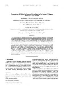
FIG. 1. Location of Lanjiang catchment and the hydrometeorological stations.
methodology, including the experimental design, the hydrological models, the bias correction method for the regional climate model outputs, the peak flow extraction approach, and the postprocessing methods for peak flows, is described in section 3. In section 4, the results and discussion on the calibration and validation of the hydrological models, the bias correction of the PRECIS predictions, the calibration and validation of the postprocessing models, and the peak flow estimation under climate change are presented. Conclusions are drawn in section 5.
2. Study area and data The study area, Lanjiang catchment, is located in the upstream part of the Qiantang River basin, east China. The catchment, contributing to about two-thirds of the runoff to the downstream Qiantang River basin, has an area of about 19 460 km2 and a main stream of about 300 km in length. The catchment is dominated by a subtropical humid monsoon climate. The annual mean rainfall is about 1600 mm and the annual mean temperature is about 178C. Peak flows usually occur during the period May–July, sometimes resulting in big floods and leading to enormous economic losses. Figure 1 shows the location of Lanjiang catchment and the hydrometeorological stations in the study area. Table 1 shows detailed information about the hydrometeorological stations. In this study, there are three discharge stations, namely, Quzhou, Jinhua, and Lanxi. Other data, such as precipitation and temperature data, are used as input for the hydrological models. In this paper, two GCMs, namely, Hadley Centre Coupled Model, version 3 (HadCM3), from the Hadley
Centre, United Kingdom (Gordon et al. 2000), and ECHAM5 from the Max Planck Institute for Meteorology, Germany (Simmons et al. 1989), under greenhouse gas emission scenario A1B, are used as the boundary forcing for the regional climate model PRECIS developed by the Hadley Centre. Climate projections for the baseline period 1961–90 and for the future period 2011–40 covering the study area are simulated by the PRECIS model. In this study, the simulation domain of the PRECIS model is east China (Xu et al. 2014). The output data from the PRECIS model with a resolution of 25 km 3 25 km are used as simulated input data for the hydrological models after bias correction (see section 3c).
3. Methodology a. Experimental design This research investigates the postprocessing of extreme flows, comparing it with a composite objective calibration of the hydrological model to improve the simulation of peak flows under climate change. Figure 2 shows the framework of this study, primarily consisting of four steps. Step 1 is about the setup of the hydrological models in the study area. Two hydrological models [SWAT and modèle du Génie Rural à 4 paramètres Journalier (GR4J)] are applied and 10 yr of daily discharges are used to calibrate and validate these models. The first 7 yr (1981–87) are used for calibration and the last 3 yr (1988–90) are used for validation. The year of 1980 is used as the warm-up period for the hydrological models. Step 2 is about the bias correction of the outputs of the PRECIS model by using the method of QM, which will be introduced later. The outputs from the
2190
JOURNAL OF HYDROMETEOROLOGY
VOLUME 16
TABLE 1. Information of the hydrometeorological stations in Lanjiang catchment.
No.
Station
Lat (8N)
Lon (8E)
Elev (m MSL)
Observed variables*
Time period
1 2 3 4 5 6 7 8 9 10 11 12 13 14 15 16 17 18 19 20 21 22 23
Jinhua Quzhou Lanxi Bada Changshan Dushan Longyou Misai Yiwu Yongkang Zhengzhai Baishuikeng Dongyang Jiangshanwanyao Nanjiangshuiku Qianhe Xujiacun Yanxi Quxiandazhou Bukengkou Darifan Kaihua Jiangshan
29.12 29.00 29.22 29.20 28.92 28.42 29.05 29.18 29.30 28.90 28.90 28.42 29.27 28.68 29.15 28.85 28.98 29.33 28.87 28.90 28.57 29.13 28.75
119.65 118.90 119.47 120.50 118.50 118.98 119.17 118.40 120.07 120.02 119.63 118.60 120.22 118.67 120.43 118.78 118.13 118.32 118.98 119.13 118.88 118.40 118.63
62.6 82.4 58 332 145 705 54 313 62 194 152 459 81 141 242 74 675 286 131 97 243 155.3 95.3
P, T, H, R, W, and Q P, T, H, R, W, and Q P and Q P P P P P P and T P and T P P P and T P P P P P P P P T T
1961–2000 1961–2000 1975–2000 1967–2000 1961–2000 1961–78, 1981–95 1980–95 1961–96 1961–2000 1961–2000 1980–95 1975–2000 1961–2000 1975–2000 1971–2000 1961–2000 1961–2000 1963–2000 1961–2000 1961–2000 1979–91 1961–2000 1961–2000
* Precipitation, P; temperature, T; humidity, H; radiation, R; wind speed, W; and discharge, Q.
PRECIS model for both the baseline period (1961–90) and the future period (2011–40) are bias corrected before being used as input for the hydrological models. Step 3 is about the simulation of peak flows by combining hydrological models and the peaks-over-threshold (POT) method to simulate daily discharges and extract peak flows. Besides the observed peak flows, there are three types of simulated peak flows using three groups of input data: the observed data from the hydrometeorological stations in the period of 1961–2000, PRECIS predictions in the baseline period, and PRECIS predictions in the future period. Step 4 is about the postprocessing of peak flows. Observed peak flows and simulated peak flows with observed input data are used to set up the postprocessing model in three ways, namely, based on the QM method and two generalized linear models (GLMs). The first 30 yr (1961–90) are used for calibration and the last 10 yr (1991–2000) are used for validation. Then the simulated peak flows with simulated input data under climate change are bias corrected by applying the postprocessing model. The composite objective calibrated GR4J model, marked as GR4J-M, takes both the daily flows and peak flows into calibration process. The peak flows are also extracted by the POT method. The simulated peak flows by the GR4J-M model will not be postprocessed,
because the model has already improved the peak flow simulation performance.
b. Hydrological models 1) MODEL DESCRIPTION The two hydrological models included in this paper are a distributed model (SWAT) and a lumped model (GR4J). These two models are well known, and details of the model structure have been widely presented in many previous studies. Below, only brief descriptions of the two models are provided. GR4J-M is actually a composite objective GR4J model combined with the POT method, including peak flows into the model calibration, which will be introduced later. The SWAT model (Arnold et al. 1998; Srinivasan et al. 1998) is a physically based distributed hydrological model, which is widely used all over the world (Abbaspour et al. 2007; Setegn et al. 2011; Strauch et al. 2012; Yang et al. 2008). The model divides a river basin into several subbasins, and each subbasin usually contains several hydrologic response units (HRUs). An HRU, the smallest unit in the SWAT model, is defined as an area with the same soil type and land-use type. Generally, the model requires the user to build the land-use database, soil database, and weather generator database for the study
OCTOBER 2015
ZHANG ET AL.
2191
FIG. 2. Methodology for postprocessing of peak flows.
area. Then the model simulates runoff with the input data such as precipitation and temperature. The GR4J model (Perrin et al. 2003) is a daily fourparameter lumped rainfall–runoff model, which is an improved version of the GR3J model. Because of its good performance in streamflow simulation, the GR4J model has been widely used all over the world (Demirel et al. 2013; Thyer et al. 2009; Tian et al. 2013). The model structure is based on a production store, a routing store, and two unit hydrographs. The required input data include the area of the catchment, daily precipitation, and potential evapotranspiration. The potential evapotranspiration is calculated using the Penman–Monteith equation (Allen et al. 1998).
2) MODEL CALIBRATION The calibration of the SWAT model is based on the software SWAT-CUP (Faramarzi et al. 2009; Schuol et al. 2008; Yang et al. 2008), which is a freely available program for sensitivity analysis, calibration, validation, and uncertainty analysis for the SWAT model. There are several calibration methods available in SWATCUP, including SUFI-2 (Sequential Uncertainty Fitting, version 2), GLUE (Generalized Likelihood Uncertainty Estimation), MCMC (Markov Chain Monte Carlo), and PSO (Particle Swarm Optimization). Yang et al. (2008) compared five calibration methods in SWAT-CUP, showing that the SUFI-2 method is an
2192
JOURNAL OF HYDROMETEOROLOGY
VOLUME 16
TABLE 2. Calibrated parameters in the SWAT model. Optimal value Parameter v__CH_K2.rte a__CN2.mgt
v__ALPHA_BF.gw v__GWQMN.gw v__GW_REVAP.gw v__ESCO.hru v__RCHRG_DP.gw r__SOL_AWC.sol r__SOL_Z.sol v__SURLAG.bsn
Definition
Initial range*
Effective hydraulic conductivity in main channel alluvium (mm h21) Initial U.S. Department of Agriculture (USDA) Soil Conservation Service (SCS) runoff curve number for moisture condition II Baseflow alpha factor (days) Threshold depth of water in the shallow aquifer required for return flow to occur (mm H2O) Groundwater ‘‘revap’’ coefficient Soil evaporation compensation factor Deep aquifer percolation fraction Available water capacity of the soil layer (mm H2O per mm soil) Depth from soil surface to bottom of layer (mm) Surface runoff lag coefficient
Quzhou
Jinhua
15.39
7.27
142.85
21.83
242.24
236.81
0.59 2881.58
0.85 2465.11
0.85 4673.13
[0.02, 0.2] [0.01, 1] [0, 1] [21, 0.8]
0.02 0.95 0.67 20.53
0.14 0.94 0.43 20.75
0.05 0.18 0.96 0.43
[21, 0.8]
20.87
20.65
20.97
2.13
2.13
2.13
[0, 150] [255, 15]
[0, 1] [0, 5000]
[1, 24]
Lanxi
* The initial ranges for different aggregate parameters are mainly based on their physically meaningful absolute ranges in the SWAT model manual and their initial values in model databases.
easy and efficient one, and it is therefore employed in this study to calibrate the SWAT model. The SUFI-2 method contains several steps that were introduced in the work of Abbaspour et al. (2004, 2007). Table 2 presents the parameters for calibration in the SWAT model following the initial parameter sensitivity analysis. As there are only four parameters in the GR4J model and the model often has a good performance with a simple calibration method, in this study, Monte Carlo simulation (MCS) with Latin Hypercube sampling for a sample size of 10 000 parameter sets is carried out. The initial parameter ranges are presented in Table 3 and the objective function for model calibration is the Nash–Sutcliffe coefficient. For the GR4J-M model, a composite objective function is used, taking into account two objectives, the Nash–Sutcliffe coefficient for daily streamflows and the Nash–Sutcliffe coefficient for peak flows. To equally weight the simulation performance for daily and extreme conditions, the weights for these two Nash–Sutcliffe coefficients are set to 0.5 and
the combined Nash–Sutcliffe coefficient NScom is defined as follows: 9 8 N > > > 2> > > > å [Qobs (i) 2 Qsim(i)] > = < NScom 5 0:5 3 1 2 i51 N > > > > > > > å [Qobs(i) 2 Qobs (i)]2 > ; : i51 8 9 M > > > > 2 > > > å [QP,obs (i) 2 QP,sim (i)] > < = i51 , (1) 1 0:5 3 1 2 M > > > 2> > > > > [Q (i) 2 Q (i)] å P,obs : ; P,obs i51
where N and M are the number of the daily flows and peak flows, respectively; Qobs and Qsim are the observed and simulated daily flows, respectively; and QP,obs and QP,sim are the observed and simulated peak flows, respectively, extracted from the daily streamflows by the POT method (see section 3d).
TABLE 3. Calibrated parameters in the GR4J and GR4J-M models. Optimal value (GR4J)
Optimal value (GR4J-M)
Parameter
Definition
Initial range
Quzhou
Jinhua
Lanxi
Quzhou
Jinhua
Lanxi
X1 X2 X3
Max capacity of the production store (mm) Groundwater exchange coefficient (mm) One day ahead max capacity of the routing store (mm) Time base of unit hydrograph UH1 (days)
[100, 1200] [25, 3] [20, 300]
141.07 0.10 44.69
284.40 20.36 28.80
235.62 0.07 38.49
115.45 0.23 31.77
144.95 0.01 44.64
139.69 20.24 22.24
2.14
2.37
2.46
2.10
2.01
2.52
X4
[1.1, 2.9]
OCTOBER 2015
ZHANG ET AL.
Besides the Nash–Sutcliffe coefficient, one other criterion is calculated to evaluate the performance of the models after calibration, the relative Bias: N
å [Qsim (i) 2 Qobs (i)]
Bias 5 i51
N
3 100%
(2)
å Qobs (i)
i51
c. Bias correction of PRECIS predictions The QM method is a statistical approach originating from the empirical transformation of Panofsky and Brier (1968). It has been successfully used for bias correction of meteorological outputs from GCMs and RCMs (Gudmundsson et al. 2012; Li et al. 2010; Themeßl et al. 2012) and also for postprocessing of hydrological forecasts (Hashino et al. 2007; Madadgar et al. 2014). The QM method is capable of correcting errors in variability because it corrects errors in the shape of the distribution. This method has been demonstrated to provide reasonable improvements in the representation of precipitation outputs on a daily, monthly, and annual level (J. Chen et al. 2013). In this study, the QM method is based on the empirical cumulative distribution function (ecdf) of daily observed and PRECIS-projected variables in the baseline period. The theoretical cumulative distribution function estimates the probability of precipitation by using wet days only, while the QM method takes both wet and dry days into account when employing the ecdfs. Therefore, the frequency of precipitation occurrence is also corrected together with the precipitation amount. By using ecdfs, the QM method is applicable to all possible output variables from the PRECIS model. The transformation function of the QM method is defined as Y 5 ecdf 21 obs [ecdf sim (X)] , CF 5 Y 2 X ,
(3) (4)
and Yfuture 5 Xfuture 1 CF,
(5)
where X is the simulated variable from the PRECIS model in the baseline period and Y is the bias-corrected value of the corresponding variable X in the baseline period. The function ecdfsim is the ecdf of the simulated variable based on the dataset in the baseline period, while the function ecdf 21 obs is the inverse ecdf of the observed variable based on the dataset in the baseline period. The bias-corrected value of the simulated variable in the future period Yfuture is estimated by adding a
2193
correction factor (CF) to the simulated variable in the future period Xfuture, and CF is defined as the difference between the bias-corrected value and the simulated raw value of the variable in the baseline period. In this study, precipitation and temperature from the PRECIS model are bias corrected both in the baseline period and the future period. As the outputs of the PRECIS model are provided at a gridcell level, the observed dataset from the nearest station to the gridcell center is used to set up ecdf 21 obs for the simulated dataset of the corresponding grid cell.
d. Peak flow extraction There are several types of flood peak series, and the widely used two types are annual maximum flood (AMF) series and POT series. The AMF series can be simply constructed by extracting the maximum daily discharge in each year, while the POT series consists of peak flows above a threshold. The POT series allow for more peaks to be selected and included in extreme flow analysis, as shown by, for instance, Parent and Bernier (2003) and Villarini et al. (2011). Application of the AMF method, naturally leads to peak flows that are independent. For the POT series, however, meeting the independence condition has to be taken into account when determining the threshold. In this study, the independence condition for peak flows proposed by the United States Water Resources Council (USWRC 1976) is employed. It suggests that two consecutive peak flows P1 and P2 are independent if 1) the time between them is larger than five days plus the natural logarithm of the basin area in square miles and 2) the intermediate flows between these two consecutive peaks must drop below 75% of the lowest of these two peak flows. Based on this independence condition, a maximum of 90 peaks in the baseline period (1961–90) are selected to set up the postprocessing model, and 30 peaks in the period 1991– 2000 are selected to validate the postprocessing model. Similarly, a maximum of 90 peaks in the future period (2011–40) are selected for the postprocessing model application. As the daily discharge record at Lanxi station is from the year of 1975, only a maximum of 48 peaks in the period 1975–90 are selected for model calibration at this station.
e. Postprocessing methods for peak flows In this study, three methods for postprocessing are compared: two types of the GLM and the QM method, which has also been used for the bias correction of PRECIS outputs. The GLM is a flexible generalization of an ordinary linear model and has been used for rainfall analysis (Chandler and Wheater 2002; Segond et al. 2006) and streamflow postprocessing (Zhao et al.
2194
JOURNAL OF HYDROMETEOROLOGY
VOLUME 16
TABLE 4. Hydrological model performance in the calibration and validation periods at Quzhou, Jinhua, and Lanxi stations. SWAT
GR4J
GR4J-M
Period
Index
Quzhou
Jinhua
Lanxi
Quzhou
Jinhua
Lanxi
Quzhou
Jinhua
Lanxi
Calibration (1981–87)
NS Bias (%) NS Bias (%)
0.74 24.1 0.78 24.0
0.76 216.9 0.76 218.5
0.76 214.2 0.78 214.3
0.94 24.9 0.95 25.2
0.91 29.1 0.91 216.7
0.92 25.8 0.95 211.2
0.91 21.2 0.91 21.5
0.84 2.3 0.88 26.1
0.89 211.1 0.92 214.7
Validation (1988–90)
2011). There are three components in the GLM, namely, the dependent variable Y, the independent variable X, and a link function g to connect them. The model expression is as follows g(m) 5 Xb 5
n
å bi xi ,
(6)
i50
where m 5 E(Y) is the expected value of Y, X is the linear predictor, b is the unknown parameter, n is the number of predictors, and g is the link function. The outcome of the dependent variable Y is assumed to be generated from a particular distribution as, for instance, the normal, binomial, Poisson, and gamma distributions. The link function provides the relationship between the expected value of the dependent variable and the linear predictors. There are many commonly used link functions, including identity, inverse and log regressions, etc. In this study, the extracted observed and simulated peak flows after sorting in ascending order are regarded as the dependent variable and independent variable, respectively, to set up the GLM. Several link functions and several distributions for the dependent variable are tested, and the parameters b are calibrated by the maximum likelihood approach. Based on the performances of different GLMs, two GLMs are finally selected. These are GLMNI and GLMGI based on the normal and gamma distributions, respectively, with the link function identity. After the calibration and validation of the postprocessing methods, the future peak flows extracted from the simulated daily flows by the SWAT and GR4J models are bias corrected by the postprocessing methods. The GR4J-M model is calibrated both on the daily flows and peak flows, and therefore the extracted future peak flows from the GR4J-M model are not bias corrected by the postprocessing methods.
4. Results and discussion a. Calibration and validation results of the hydrological models Tables 2 and 3 also show the calibrated values for the parameters in the SWAT model and the GR4J and GR4J-M models, respectively. Table 4 presents the results of the two model performance indices in the
calibration and validation periods for the three hydrological models for the three discharge stations. Based on the values of the objective function NS, the SWAT model performance is worse than the other two models. Besides the differences between model structures, this might be related to the different calibration methods. Other studies such as Zhang et al. (2009) show that the genetic algorithms (GA) and PSO methods are preferred based on different numbers of model runs. As the GR4J-M model includes peak flows into model calibration, it shows a worse performance than the GR4J model in terms of daily discharges. The NS values in the validation period are slightly higher than those in the calibration period. This is mainly because the variance of observed discharges in the validation period is much larger than that in the calibration period (the variances in the validation period are 69%, 92%, and 73% larger than those in the calibration period at Quzhou, Jinhua, and Lanxi stations, respectively), increasing the NS values. In general, the three models underestimate the daily discharges according to the values of Bias, particularly for Jinhua and Lanxi stations in the SWAT model. According to the two evaluation indices, the model performance is the best at Quzhou station for all three hydrological models, indicating that the watershed characteristics also play a significant role in streamflow simulation, as well as the hydrological model structure. In general, the NS values are all higher than 0.7 for the SWAT model and higher than 0.8 for the other two lumped models, which is considered as a satisfactory performance for a daily step simulation. Figure 3 shows the flow duration curves of observed and simulated daily flows in the calibration period at Quzhou, Jinhua, and Lanxi stations. For the purpose of comparing the peak flows clearly, the range of the x axis is set to [0, 10]. It can be seen that the GR4J model is better than the SWAT model in terms of peak flow simulation, but there is still some underestimation of peak flows, especially at Jinhua and Lanxi stations. Actually, there are on average three peak flows per year extracted by the POT method in this study. Excluding the peak flows that do not satisfy the independence condition in POT method, the exceedance quantile of the extracted peak flows in Fig. 3 is about 1%. With
OCTOBER 2015
ZHANG ET AL.
2195
FIG. 3. Flow duration curves of daily observed discharges (OBS) and simulated discharges by the SWAT, GR4J, and GR4J-M models in the calibration period 1981–87 at three stations: (a) Quzhou, (b) Jinhua, and (c) Lanxi.
regard to the simulation of the 1% peak flows, the GR4J-M model performs better than the GR4J model because of the composite objective in the calibration process. Recently, there have been some studies focusing on quantifying the impact of human activities on runoff in the SWAT model (e.g., Fan et al. 2010; A. Zhang et al. 2012; C. Zhang et al. 2012). They aim to distinguish the impact caused by climate change and human activities in the historical period. However, in the future period, it is difficult to model the impact of human activities. To some extent, human activities have already been incorporated in climate change scenarios based on CO2
emissions. Therefore, human activities are not considered in the SWAT model in this study. Besides, some other studies such as Zhang et al. (2013) have investigated the interactions among different parameters in the SWAT model using Sobol’s method, which is a good approach for sensitivity analysis and to improve parameter calibration.
b. Bias correction results of the PRECIS model The daily precipitation and maximum and minimum temperature at the hydrometeorological stations in the baseline and future periods projected by the PRECIS model are bias corrected by the QM method. To
2196
JOURNAL OF HYDROMETEOROLOGY
VOLUME 16
FIG. 4. The ecdfs of the observed, PRECIS-simulated—under (left) HadCM3 and (right) ECHAM5—, and biascorrected daily precipitations in the baseline period 1961–90 at three stations: (a),(b) Quzhou; (c),(d) Jinhua; and (e),(f) Lanxi.
evaluate the performance, the observed, simulated, and bias-corrected precipitations in the baseline period are compared and three hydrometeorological stations (i.e., Quzhou, Jinhua, and Lanxi) are taken as examples to show the results of bias correction. Figure 4 shows the ecdfs of the daily precipitation at these three stations in the baseline period. For the purpose of presenting the
ecdfs clearly, the ranges of the x and y axes are set to [0, 80] and [0.6, 1], respectively. For Quzhou and Jinhua stations, a large number of daily precipitation values smaller than 80 mm are underestimated, while for Lanxi station, they are overestimated. After bias correction, at all three stations, the ecdfs of simulated daily precipitation become very close to those of observed daily
OCTOBER 2015
ZHANG ET AL.
2197
FIG. 5. Annual max precipitation extracted from observed, PRECIS-simulated—under (left) HadCM3 and (right) ECHAM5—, and biascorrected daily precipitation in the baseline period 1961–90 at three stations: (a),(b) Quzhou; (c),(d) Jinhua; and (e),(f) Lanxi.
precipitation, demonstrating a very satisfactory performance of the QM bias correction method. As this study focuses on peak flows, the bias correction performance is also evaluated for extreme precipitation values, which are the driving forces for peak flows. Figure 5 shows the observed, PRECIS model–simulated, and QM
bias-corrected annual maximum precipitation in the baseline period at the three example stations. At all three stations, the annual maximum precipitation with a small exceedance probability simulated with HadCM3 boundary data are larger than those simulated with ECHAM5 boundary data, while an opposite situation is
0.97 20.6 0.94 23.5 0.996 0 0.93 27.7 0.996 0 0.93 27.9 0.999 20.2 0.91 27.8 0.98 213.4 0.75 220.6 0.96 1.5 20.57 16.5 0.98 0 0.61 5.6 * The subscript P in the two indices stands for peak flows.
0.67 255.0 20.27 249.9 NSP BiasP (%) NSP BiasP (%)
0.999 20.4 0.91 20.7
0.97 20.5 0.81 12.4 0.97 20.4 0.94 26.1 0.97 0 0.95 25.3 0.99 20.9 0.93 25.0 0.56 227.3 0.30 231.3 0.94 20.8 0.66 16.3 0.96 0 0.36 21.2 0.02 240.6 0.38 230.6 NSP BiasP (%) NSP BiasP (%)
0.99 21.2 0.68 14.6
0.96 0.9 0.94 23.9 0.99 20.2 0.94 8.5 0.99 0 0.93 9.5 0.996 20.6 0.96 7.3 0.82 216.2 0.92 29.5 0.89 1.2 0.78 22.3 0.95 0 0.79 26.5 20.33 248.2 20.28 250.2 NSP BiasP (%) NSP BiasP (%)
0.998 20.6 0.90 24.6
VOLUME 16
Quzhou Calibration (1961–90) Validation (1991–2000) Jinhua Calibration (1961–90) Validation (1991–2000) Lanxi Calibration (1975–90) Validation (1991–2000)
GLMGI GLMNI
GR4J
QM Raw GLMGI SWAT
GLMNI QM Raw
Three approaches (i.e., QM, GLMNI, and GLMGI) are applied to set up the postprocessing models to correct the biases in the peak flows extracted from daily flows simulated by the SWAT and GR4J models at Quzhou, Jinhua, and Lanxi stations. The two indices (i.e., Nash–Sutcliffe coefficient and relative bias) are also used in this subsection to evaluate the performance of the postprocessing models. Table 5 shows the values of Nash–Sutcliffe coefficient (NSP ) and relative bias (BiasP ) for the raw and bias-corrected peak flows in the calibration and validation periods at these three stations. Compared with the raw peak flows simulated by the SWAT and GR4J models, obvious improvements in the simulation of bias-corrected peak flows by all three postprocessing models can be observed both in the calibration and validation periods at Quzhou station,
Index*
c. Calibration and validation results of postprocessing models
Period
shown for precipitation with a large exceedance probability, indicating larger variability exists in the annual maximum precipitation values simulated with HadCM3 boundary data than those simulated with ECHAM5 boundary data. At Quzhou station, most annual maximum precipitation values are underestimated, except several extreme precipitation values simulated with HadCM3 boundary data. At Jinhua station, however, most annual maximum precipitation values are overestimated, except several precipitation values with a large exceedance probability simulated with HadCM3 boundary data. At Lanxi station, all annual maximum precipitation values are overestimated by the PRECIS model both with HadCM3 and ECHAM5 boundary data, and biases are much larger, in accordance with the results in Figs. 4e and 4f. Overall, the bias-corrected annual maximum precipitation values are quite close to the observed ones at all three stations, confirming the satisfactory performance of the QM bias correction method. As J. Chen et al. (2013) stated, compared with the change factor method, the advantage of the QM method is that the future precipitation occurrence is also corrected along with the magnitude. This is very important in some temperate basins such as our study area, because an extreme flood is usually caused by one or a few extreme rainfall events. However, the QM method may underestimate the interannual variability in some way. In the areas where there is obvious interannual variability in climate or the temporal dependence is significant, one can refer to some other bias correction methods that take temporal dependence into account, such as the nested bias correction proposed by Johnson and Sharma (2012).
GR4J-M Raw
JOURNAL OF HYDROMETEOROLOGY TABLE 5. Model performance of raw simulated, postprocessed, and composite objective calibrated peak flows in the calibration and validation periods at Quzhou, Jinhua, and Lanxi stations.
2198
OCTOBER 2015
ZHANG ET AL.
2199
FIG. 6. Peak flows of observed (OBS), simulated by hydrological models (Raw)—under (left) SWAT, (middle) GR4J, and (right) GR4JM—, and bias-corrected by three postprocessing methods (GLMGI, GLMNI, and QM) in the calibration period at three stations: (a)–(c) Quzhou, (d)–(f) Jinhua, and (g)–(i) Lanxi.
especially for the SWAT model. At Jinhua station, similar improvements can be observed in the postprocessed peak flows, except for the GLMNI postprocessing model when applied to the SWAT-simulated peak flows in the validation period in terms of the two evaluation indices. At Lanxi station, except for the GLMGI postprocessing model when applied to the SWAT-simulated peak flows in the validation period (with a NSP value of 20.57), simulation of all other peak flows is improved by the postprocessing models to a large extent. When applied to the GR4J-simulated peak flows, all three postprocessing models perform nicely both in the calibration and validation periods. Since the GR4J-M model is calibrated with a composite objective function by taking peak flows into account, the raw peak flows simulated by the GR4JM model have a performance comparable with the other postprocessed peak flows at all three stations both in the calibration and validation periods. Figure 6 shows the observed, simulated, and biascorrected peak flows in the calibration period at
Quzhou, Jinhua, and Lanxi stations. The raw peak flows simulated by the SWAT and GR4J models all underestimate the observed peak flows, and the biases are larger for the SWAT than for the GR4J model. At Quzhou station, the postprocessing models perform well in correcting the biases in the raw peak flows simulated by the SWAT and GR4J models, except an apparent overestimation for the highest peak in the GLMGI postprocessing model when applied to the SWATsimulated peak flows in Fig. 6a. The peak flows are also well simulated by the GR4J-M model, as can be seen in Fig. 6c. At Jinhua station, it can be observed that all peak flows are well simulated by the postprocessing models and the GR4J-M model. At Lanxi station, it can be observed that the GLMGI model obviously overestimates the highest peak when applied to the raw peaks simulated by the SWAT model, similar to Quzhou station. Other postprocessed peak flows perform considerably well, as do the peak flows simulated by the GR4J-M model.
2200
JOURNAL OF HYDROMETEOROLOGY
VOLUME 16
FIG. 7. As in Fig. 6, but for the validation period.
Figure 7 shows the observed, simulated, and biascorrected peak flows in the validation period at Quzhou, Jinhua, and Lanxi stations. It can be observed that almost all raw peak flows simulated by the SWAT and GR4J models are underestimated at all three stations. The performance of all three postprocessing models is worse in the validation period than in the calibration period. However, except some overestimations of high peaks by all three postprocessing models when applied to the raw peak flows simulated by the SWAT model, other peak flows are reasonably well simulated, as seen in Figs. 7a, 7d, and 7g. For the postprocessing models applied to raw peak flows simulated by the GR4J model, performances are more satisfactory based on Figs. 7b, 7e, and 7h. Furthermore, it can be observed from Figs. 7c, 7f, and 7i that the GR4J-M model performs well in the validation period, especially at Lanxi station. In general, the performances of the postprocessing models in the calibration and validation periods are satisfactory and only a few peak flows are not postprocessed well by the GLMGI or GLMNI models. The QM postprocessing model is the best one among the
three models and can correct the biases in the raw peak flows significantly, especially for the SWAT-simulated peak flows. Based on the performance of the GR4J-M model, it can be concluded that using a composite objective function to take peak flows into account in the calibration process of a hydrological model is also an effective way to improve the accuracy in the simulation of peak flows. For a lumped hydrological model such as the GR4J model, the composite objective calibration taking peak flows into account is a good alternative to improve the simulation performance of peak flows, as it is much easier to combine another objective function into the model calibration process. However, it should be noticed that composite objective calibration will probably weaken the simulation performance of daily flows to some extent. For a distributed hydrological model such as the SWAT model, it is much easier to employ a postprocessing model to improve the peak flow simulation, since it is a cumbersome process to combine peak flows into the model calibration process. Comparing two approaches, the postprocessing approach is based on a statistical analysis of the difference
OCTOBER 2015
ZHANG ET AL.
2201
FIG. 8. As in Fig. 6, but for observed inputs (Raw) and PRECIS-simulated inputs with ECHAM5 and HadCM3 boundary conditions (Raw_ECHAM5 and Raw_HadCM3) in the baseline period 1961–90.
between the simulated and observed peak flows, while the composite objective calibration combines two calibration goals during the simulation of the peak flows. The postprocessing approach can be understood as a blind adjustment of the errors existing in the simulated peak flows. It can be argued that the postprocessing approach is not physically based, but it must be admitted that the approach works. This is why the postprocessing approach has been widely used (Madadgar et al. 2014; Van Andel et al. 2013; Zhao et al. 2011). Furthermore, a statistically based approach may provide a clue and a driving force for scientists to find the physically based relationship that remains under cover. The composite objective calibration can improve the accuracy of peak flow simulation, but it may offset the accuracy of daily flow simulation in the meanwhile. This is confirmed in Table 4 as the NS values for daily flows of the GR4J-M model are lower than those of the GR4J model. It is important to notice the trade-off when choosing the objective functions. The postprocessing approach can be used as a flexible alternative to composite objective
calibration of distributed hydrological model, which is often cumbersome and time consuming.
d. Comparison of simulated peak flows with different inputs In this study, the simulations of peak flows with observed and simulated inputs are evaluated in the baseline period to investigate the input data quality under climate change projection. Figure 8 shows the peak flows simulated by the SWAT, GR4J, and GR4J-M models with observed inputs and PRECIS-simulated inputs with ECHAM5 and HadCM3 boundary data in the baseline period 1961–90. It can be observed that most peak flows simulated by the hydrological models with PRECIS-simulated inputs are very close to those simulated with observed inputs. The PRECIS-simulated precipitation and temperature are bias corrected by the QM method before being used in the hydrological models. However, more significant variability that cannot be reflected in the ecdf may exist in the projected precipitation by climate models. Based on Fig. 8, it can
2202
JOURNAL OF HYDROMETEOROLOGY
FIG. 9. Correlation coefficient between observed peak flows and observed precipitation amounts at different temporal scales in days in the baseline period at Quzhou, Jinhua, and Lanxi stations.
be demonstrated that the variability only slightly affects the peak flows simulated by the hydrological models, because biases between the simulated peak flows with observed and PRECIS-simulated inputs are not very large, except those simulated by the SWAT model at Quzhou and Lanxi stations. Therefore, it can be concluded that using GR4J and GR4J-M models is appropriate for simulating peak flows under climate change, while the SWAT model may overestimate the peak flows with projected precipitation and temperature by climate models at Quzhou and Lanxi stations. It can also be observed from Fig. 8 that high-peak flows (in the tail) simulated with HadCM3 boundary data are larger than those simulated with ECHAM5 boundary data. Figure 5 shows that after bias correction, the maximum daily precipitation predicted by the PRECIS model with both HadCM3 and ECHAM5 boundary data are very close to the observed ones in the baseline period. However, one peak flow in day i may be more related to the rainfall amounts in several consecutive N days (from day i 2 N 1 1 to day i) rather than the daily rainfall in day i. The number N is usually related to catchment characteristics such as size and slope. Figure 9 shows the correlation coefficient between observed peak flows and observed precipitation at different temporal scales in the baseline period at Quzhou, Jinhua, and Lanxi stations. It can be observed that the correlation coefficient for Quzhou station increases sharply with N, varying from 1 to 4, and then becomes relatively stable. The correlation coefficients for Jinhua and Lanxi stations reach the crest value when N is 3. Therefore, it is concluded that the peak flows are more related to precipitation amounts in four consecutive days at Quzhou station and three consecutive days at Jinhua and Lanxi stations rather than the daily precipitation amount.
VOLUME 16
Figure 10 shows maximum precipitation over four consecutive days at Quzhou station and three consecutive days at Jinhua and Lanxi stations calculated based on the observed, PRECIS-simulated, and bias-corrected daily precipitation in the baseline period. Although the daily precipitation is bias corrected, it can be observed from Fig. 10 that there are small biases in the extreme heavy precipitation in three or four consecutive days. The bias-corrected extreme heavy precipitation in three or four consecutive days simulated with HadCM3 boundary data is larger than those simulated with ECHAM5 boundary data at all three stations. This is why the extreme high-peak flows simulated with HadCM3 boundary data are larger than those simulated with ECHAM5 boundary data presented in Fig. 8. Overall, most precipitation in three or four consecutive days simulated by the PRECIS model perform well after bias correction in accordance with the observed ones. The peak flows simulated by the hydrological models with PRECIS-simulated inputs also perform well in accordance with those simulated with observed inputs, especially for the GR4J and GR4J-M models (see Fig. 8). Therefore, it is appropriate to simulate future peak flows using projected climate data as hydrological model inputs. It should be kept in mind that based on Fig. 8, the SWAT model may overestimate future peak flows at Quzhou and Lanxi stations, and future extreme high-peak flows may be underestimated with ECHAM5 boundary data while overestimated with HadCM3 boundary data at Lanxi station.
e. Postprocessing results of peak flows under climate change In this study, the peak flows are simulated with projected climate data and then bias corrected by the postprocessing model both in the baseline period 1961– 90 and the future period 2011–40 to investigate the impact of climate change on peak flows in Lanjiang catchment. The final postprocessing (PP) model is chosen to be an ensemble model of the three methods GLMNI, GLMGI, and QM and is defined as a simple linear combination of the three methods. As the QM method performs better than the other two, the weights in the PP model are set to 1/ 4, 1/ 4, and 1/ 2 for GLMNI, GLMGI, and QM, respectively. Although the choice of weights seems a little arbitrary here, this will not affect the main conclusion of this study. More solid methods of choosing the weights can refer to other works (e.g., Cooper et al. 2007; Liang et al. 2011). There are three models to estimate the peak flows under climate change in this study, namely, the SWAT model combined with the postprocessing model (SWAT-PP), the GR4J model combined with the postprocessing model (GR4J-PP), and the GR4J-M model.
OCTOBER 2015
ZHANG ET AL.
2203
FIG. 10. Annual max precipitation in four consecutive days at (a),(b) Quzhou and three consecutive days at (c),(d) Jinhua and (e),(f) Lanxi calculated from observed, PRECIS-simulated—under (left) HadCM3 and (right) ECHAM5—, and bias-corrected daily precipitation in the baseline period 1961–90.
Figure 11 shows the peak flows simulated by the three models with PRECIS-projected input data under HadCM3 and ECHAM5 boundary conditions both in the baseline period and the future period at Lanxi station taken as an example. For small peak flows simulated
by SWAT-PP with HadCM3 boundary data at Lanxi station in Fig. 11a, the differences between the baseline peak flows and future peak flows are very small. However, when peak flows increase, the differences become large. The future extreme high-peak flows estimated by
2204
JOURNAL OF HYDROMETEOROLOGY
VOLUME 16
FIG. 11. Simulated peak flows by the hydrological models—(top) SWAT, (middle) GR4J, and (bottom) GR4J-M— with projected input data from the PRECIS model under (left) HadCM3 and (right) ECHAM5 boundary conditions (Raw) and the postprocessed peak flows (PP) both in the baseline period 1961–90 (BSL) and the future period 2011–40 (FUT) at Lanxi station.
the three models are all much larger than those in the baseline period. Furthermore, an overall trend can be observed that extreme high-peak flows simulated by all three models under HadCM3 boundary conditions are much larger than those under ECHAM5 boundary
conditions. This indicates that HadCM3 simulates more extreme precipitation in Lanjiang catchment than the ECHAM5 model, as the extreme high flows are usually caused by extreme precipitation as shown in Fig. 10.
OCTOBER 2015
2205
ZHANG ET AL.
TABLE 6. Comparison of three selected large peaks (m3 s21) simulated by different models in the baseline period and the future period at Quzhou, Jinhua, and Lanxi stations. HadCM3 Peak No.* Quzhou 70th
80th
90th
Jinhua 70th
80th
90th
Lanxi 70th
80th
90th
ECHAM5
Period**
SWAT-PP
GR4J-PP
GR4J-M
SWAT-PP
GR4J-PP
GR4J-M
BSL FUT Change (%) BSL FUT Change BSL FUT Change (%)
2670 3629 35.9 3335 4505 35.1 6513 11 534 77.1
1946 3783 94.4 2710 4274 57.7 5999 13 394 123.3
1859 3331 79.2 2627 3779 43.9 5583 12 932 131.6
2643 3388 28.2 2950 3833 29.9 4694 8726 85.9
1998 3443 72.3 2329 4216 81.0 4310 10 001 132.0
1946 3233 66.1 2344 4256 81.6 3928 9589 144.1
BSL FUT Change (%) BSL FUT Change (%) BSL FUT Change (%)
1754 2513 43.3 2384 3056 28.2 4698 6581 40.1
1340 2606 94.5 1533 3118 103.4 3538 6432 81.8
1326 2269 71.1 1612 2983 85.0 3779 8993 138.0
1695 2224 31.2 2160 2490 15.3 3578 4003 11.9
1291 2041 58.1 1559 2499 60.3 2526 3948 56.3
1261 2199 74.4 1411 2515 78.2 2350 4884 107.8
BSL FUT Change (%) BSL FUT Change (%) BSL FUT Change (%)
7096 9589 35.1 8977 11 792 31.4 18 459 26 547 43.8
4266 7580 77.7 6055 9185 51.7 11 747 20 731 76.5
4285 7331 71.1 5623 8802 56.5 11 290 21 137 87.2
6659 7840 17.7 7839 9737 24.2 14 121 18 365 30.1
4250 7207 69.6 5136 8726 69.9 7050 12 794 81.5
4188 6838 63.3 4658 8685 86.5 6896 11 948 73.3
* The 70th, 80th, and 90th peak flows are in accordance with Fig. 11, namely the 21st, 11th, and 1st largest peaks, respectively. ** BSL is the baseline period 1961–90 and FUT is the future period 2011–40. Change is the relative change of peak flows in the future period to the baseline period.
Table 6 shows the quantitative comparison of three selected large peaks simulated by three models in the baseline period and the future period at Quzhou, Jinhua, and Lanxi stations. The change in peak flows in the future period relative to the baseline period varies from 28.2% to 144.1% at Quzhou station, from 11.9% to 138.0% at Jinhua station, and from 17.7% to 87.2% at Lanxi station. The peak flows simulated by the three models in the future period are all larger than those in the baseline period at all three stations under both HadCM3 and ECHAM5 boundary conditions, reliably indicating that more frequent and severe floods in the future period 2011–40 in Lanjiang catchment can be expected. Decision-makers should take these changes in extreme precipitation and flows into account in order to make robust decisions regarding future construction and water management plans. In the meanwhile, it can be observed that the variability caused by three models (SWAT-PP, GR4J-PP, and GR4J-M) is larger than that
by two GCMs, indicating that the model structure and model calibration may cause large uncertainty in future peak flow projections. However, only two GCMs are used in this study, which may narrow the uncertainty due to GCM structure and parameters, since many other studies show that GCM structure is the largest uncertainty source (e.g., Kay et al. 2009; Chen et al. 2011; Woldemeskel et al. 2012). Besides, other uncertainty sources, such as downscaling methods, may also play a very important role (Sunyer et al. 2014). It is therefore proposed that a full-scale uncertainty analysis considering multiple GCMs, downscaling methods, and hydrological models is implemented in future climate change impact analyses.
5. Conclusions This study proposed a postprocessing framework to correct biases in peak flows simulated by hydrological
2206
JOURNAL OF HYDROMETEOROLOGY
models under climate change in Lanjiang catchment, the upstream part of Qiantang River basin, east China. Two hydrological models, namely, SWAT and GR4J, were set up to simulate daily flows at three stations in the catchment. The POT method was used to extract peak flows from the daily flows. Three methods, quantile mapping and two generalized linear models, were employed to correct biases in the peak flows. A composite objective calibration of the GR4J model by taking peak flows into account is also investigated to compare with the performance of the postprocessing methods. Finally, the impact of climate change on peak flows was evaluated based on the proposed framework. The following conclusions can be drawn: 1) The SWAT and GR4J models underestimate peak flows, which might be due to some specific characteristics of Lanjiang catchment or biases in observed precipitation, temperature, and discharge. This is the main motivation to set up the postprocessing model for simulated peak flows in this study. 2) The quantile mapping method shows a good performance in correcting the biases in the simulated daily precipitation by the PRECIS regional climate model. In simulating extreme precipitation, the PRECIS model with HadCM3 boundary data projects higher values than the one with ECHAM5 boundary data. 3) The three postprocessing models (GLMNI, GLMGI, and QM) can correct the biases in raw peak flows simulated by the SWAT and GR4J models effectively. Based on the calibration and validation results, the QM model is the best one among the three postprocessing models. 4) Based on the performance of the GR4J-M model in simulating peak flows, it can be concluded that combining the peak flows into a composite objective function can improve the accuracy of peak flows. However, it may weaken the performance in daily flow simulation to some extent. 5) Based on the performance of the postprocessing methods and composite objective calibration, it is hard to conclude which approach is preferred to improve the simulation of peak flows. For some lumped hydrological models such as the GR4J model, composite objective calibration is an efficient way to improve the simulation of peak flows as it is easier to combine more than one objective function into the calibration process. This is because the codes of lumped hydrological models are usually shorter and faster than distributed models, and once the objective function aiming at peak flows is combined during model calibration, postprocessing is not really necessary.
VOLUME 16
6) Future peak flows estimated by the three hydrological models (SWAT-PP, GR4J-PP, and GR4J-M) are larger than those in the baseline period, especially the most extreme high-peak flows. Although extreme precipitation may be overestimated by the PRECIS model with HadCM3 boundary data, the simulated peak flows with ECHAM5 boundary data also show an apparent increase in the future period 2011–40 at all three stations, indicating that more frequent and heavy floods in Lanjiang catchment under climate change can be expected. Up to now, there are no hydrological models that can simulate peak flows with an accuracy of 100%. The results of this study can be generalized to other hydrological models or other catchments. If there is large overestimation or underestimation in most of the simulated peak flows and the performance of the model is hard to improve during the calibration process, both the postprocessing and composite objective calibration are good alternatives to reduce the biases in the simulated peak flows. In some areas where there are large differences between high flows and low flows, then the composite objective calibration may be a priori choice. It is advisable for researchers to try the methods in this study and develop other new methods for the postprocessing and composite objective calibration of a hydrological model. Acknowledgments. The National Climate Center of China Meteorological Administration and the Bureau of Hydrology, Zhejiang Province, are acknowledged for providing the hydrometeorological data for Lanjiang catchment. The Met Office Hadley Centre is also acknowledged for providing the PRECIS model and the model boundary data (http://www.metoffice.gov. uk/precis). The authors would also like to acknowledge the financial support provided by the National Natural Science Foundation of China (51379138), Zhejiang Provincial Natural Science Foundation of China (LR14E090001), the International Science and Technology Cooperation Program of China (2010DFA24320) and China Scholarship Council (201306320104).
REFERENCES Abbaspour, K. C., C. A. Johnson, and M. T. Van Genuchten, 2004: Estimating uncertain flow and transport parameters using a sequential uncertainty fitting procedure. Vadose Zone J., 3, 1340–1352, doi:10.2113/3.4.1340. ——, J. Yang, I. Maximov, R. Siber, K. Bogner, J. Mieleitner, J. Zobrist, and R. Srinivasan, 2007: Modelling hydrology and water quality in the pre-alpine/alpine Thur watershed using SWAT. J. Hydrol., 333, 413–430, doi:10.1016/j.jhydrol.2006.09.014.
OCTOBER 2015
ZHANG ET AL.
Akhtar, M., N. Ahmad, and M. J. Booij, 2008: The impact of climate change on the water resources of Hindukush–Karakorum– Himalaya region under different glacier coverage scenarios. J. Hydrol., 355, 148–163, doi:10.1016/j.jhydrol.2008.03.015. Allen, R. G., L. S. Pereira, D. Raes, and M. Smith, 1998: Crop evapotranspiration: Guidelines for computing crop water requirements. FAO Irrigation and Drainage Paper 56, 300 pp. [Available online at www.fao.org/docrep/X0490E/X0490E00.htm.] Arnold, J. G., R. Srinivasan, R. S. Muttiah, and J. R. Williams, 1998: Large area hydrologic modeling and assessment. Part I: Model development. J. Amer. Water Resour. Assoc., 34, 73–89, doi:10.1111/j.1752-1688.1998.tb05961.x. Ault, T. R., J. E. Cole, J. T. Overpeck, G. T. Pederson, and D. M. Meko, 2014: Assessing the risk of persistent drought using climate model simulations and paleoclimate data. J. Climate, 27, 7529–7549, doi:10.1175/JCLI-D-12-00282.1. Booij, M. J., 2005: Impact of climate change on river flooding assessed with different spatial model resolutions. J. Hydrol., 303, 176–198, doi:10.1016/j.jhydrol.2004.07.013. Booth, J. F., C. M. Naud, and A. D. Del Genio, 2013: Diagnosing warm frontal cloud formation in a GCM: A novel approach using conditional subsetting. J. Climate, 26, 5827–5845, doi:10.1175/ JCLI-D-12-00637.1. Brown, J. D., and D. Seo, 2013: Evaluation of a nonparametric post-processor for bias correction and uncertainty estimation of hydrologic predictions. Hydrol. Processes, 27, 83–105, doi:10.1002/hyp.9263. Chandler, R. E., and H. S. Wheater, 2002: Analysis of rainfall variability using generalized linear models: A case study from the west of Ireland. Water Resour. Res., 38, 1192, doi:10.1029/ 2001WR000906. Chen, J., F. P. Brissette, A. Poulin, and R. Leconte, 2011: Overall uncertainty study of the hydrological impacts of climate change for a Canadian watershed. Water Resour. Res., 47, W12509, doi:10.1029/2011WR010602. ——, ——, D. Chaumont, and M. Braun, 2013: Performance and uncertainty evaluation of empirical downscaling methods in quantifying the climate change impacts on hydrology over two North American river basins. J. Hydrol., 479, 200–214, doi:10.1016/ j.jhydrol.2012.11.062. Chen, X., T. Yang, X. Wang, C. Xu, and Z. Yu, 2013: Uncertainty intercomparison of different hydrological models in simulating extreme flows. Water Resour. Manage., 27, 1393–1409, doi:10.1007/s11269-012-0244-5. Cooper, W. W., J. L. Ruiz, and I. Sirvent, 2007: Choosing weights from alternative optimal solutions of dual multiplier models in DEA. Eur. J. Oper. Res., 180, 443–458, doi:10.1016/j.ejor.2006.02.037. Cullather, R. I., S. M. J. Nowicki, B. Zhao, and M. J. Suarez, 2014: Evaluation of the surface representation of the Greenland Ice Sheet in a general circulation model. J. Climate, 27, 4835–4856, doi:10.1175/JCLI-D-13-00635.1. Demirel, M. C., M. J. Booij, and A. Y. Hoekstra, 2013: Effect of different uncertainty sources on the skill of 10 day ensemble low flow forecasts for two hydrological models. Water Resour. Res., 49, 4035–4053, doi:10.1002/wrcr.20294. Dobler, C., G. Bürger, and J. Stötter, 2012: Assessment of climate change impacts on flood hazard potential in the Alpine Lech watershed. J. Hydrol., 460–461, 29–39, doi:10.1016/ j.jhydrol.2012.06.027. DWRZJ, 2013: ‘‘Fitow’’ seriously affected the province: 17.395 billion in direct economic losses. Accessed 3 December 2013. [Available online at http://slt.zj.gov.cn/pages/document/106/ document_889.htm.]
2207
Fan, J., F. Tian, Y. Yang, S. Han, and G. Qiu, 2010: Quantifying the magnitude of the impact of climate change and human activity on runoff decline in Mian River basin, China. Water Sci. Technol., 62, 783–791, doi:10.2166/wst.2010.294. Faramarzi, M., K. C. Abbaspour, R. Schulin, and H. Yang, 2009: Modelling blue and green water resources availability in Iran. Hydrol. Processes, 23, 486–501, doi:10.1002/hyp.7160. Feddersen, H., A. Navarra, and M. N. Ward, 1999: Reduction of model systematic error by statistical correction for dynamical seasonal predictions. J. Climate, 12, 1974–1989, doi:10.1175/ 1520-0442(1999)012,1974:ROMSEB.2.0.CO;2. Field, C. B., and Coauthors, Eds., 2012: Managing the Risks of Extreme Events and Disasters to Advance Climate Change Adaptation. Cambridge University Press, 582 pp. Gordon, C., C. Cooper, C. A. Senior, H. Banks, J. M. Gregory, T. C. Johns, J. F. B. Mitchell, and R. A. Wood, 2000: The simulation of SST, sea ice extents and ocean heat transports in a version of the Hadley Centre Coupled Model without flux adjustments. Climate Dyn., 16, 147–168, doi:10.1007/s003820050010. Gudmundsson, L., J. B. Bremnes, J. E. Haugen, and T. EngenSkaugen, 2012: Technical Note: Downscaling RCM precipitation to the station scale using statistical transformations—A comparison of methods. Hydrol. Earth Syst. Sci., 16, 3383– 3390, doi:10.5194/hess-16-3383-2012. Hashino, T., A. A. Bradley, and S. S. Schwartz, 2007: Evaluation of bias-correction methods for ensemble streamflow volume forecasts. Hydrol. Earth Syst. Sci., 11, 939–950, doi:10.5194/ hess-11-939-2007. Immerzeel, W. W., L. P. van Beek, and M. F. Bierkens, 2010: Climate change will affect the Asian water towers. Science, 328, 1382–1385, doi:10.1126/science.1183188. Johnson, F., and A. Sharma, 2012: A nesting model for bias correction of variability at multiple time scales in general circulation model precipitation simulations. Water Resour. Res., 48, W01504, doi:10.1029/2011WR010464. Karnauskas, K. B., J. E. Smerdon, R. Seager, and J. F. GonzálezRouco, 2012: A Pacific centennial oscillation predicted by coupled GCMs. J. Climate, 25, 5943–5961, doi:10.1175/JCLI-D-11-00421.1. Kay, A. L., H. N. Davies, V. A. Bell, and R. G. Jones, 2009: Comparison of uncertainty sources for climate change impacts: flood frequency in England. Climatic Change, 92, 41–63, doi:10.1007/s10584-008-9471-4. Lackmann, G. M., 2013: The south-central U.S. flood of May 2010: Present and future. J. Climate, 26, 4688–4709, doi:10.1175/ JCLI-D-12-00392.1. Li, H., J. Sheffield, and E. F. Wood, 2010: Bias correction of monthly precipitation and temperature fields from Intergovernmental Panel on Climate Change AR4 models using equidistant quantile matching. J. Geophys. Res., 115, D10101, doi:10.1029/2009JD012882. Liang, H., G. Zou, A. T. K. Wan, and X. Zhang, 2011: Optimal weight choice for frequentist model average estimators. J. Amer. Stat. Assoc., 106, 1053–1066, doi:10.1198/jasa.2011.tm09478. Liu, Y., Q. Duan, L. Zhao, A. Ye, Y. Tao, C. Miao, X. Mu, and J. C. Schaake, 2013: Evaluating the predictive skill of post-processed NCEP GFS ensemble precipitation forecasts in China’s Huai River basin. Hydrol. Processes, 27, 57–74, doi:10.1002/hyp.9496. Madadgar, S., H. Moradkhani, and D. Garen, 2014: Towards improved post-processing of hydrologic forecast ensembles. Hydrol. Processes, 28, 104–122, doi:10.1002/hyp.9562. Matonse, A. H., and A. Frei, 2013: A seasonal shift in the frequency of extreme hydrological events in southern New York State. J. Climate, 26, 9577–9593, doi:10.1175/JCLI-D-12-00810.1.
2208
JOURNAL OF HYDROMETEOROLOGY
Panofsky, H. A., and G. W. Brier, 1968: Some Applications of Statistics to Meteorology. The Pennsylvania State University Press, 224 pp. Parent, E., and J. Bernier, 2003: Bayesian POT modeling for historical data. J. Hydrol., 274, 95–108, doi:10.1016/S0022-1694(02)00396-7. Perrin, C., C. Michel, and V. Andréassian, 2003: Improvement of a parsimonious model for streamflow simulation. J. Hydrol., 279, 275–289, doi:10.1016/S0022-1694(03)00225-7. Planton, S., M. Déqué, F. Chauvin, and L. Terray, 2008: Expected impacts of climate change on extreme climate events. C. R. Geosci., 340, 564–574, doi:10.1016/j.crte.2008.07.009. Safeeq, M., and A. Fares, 2012: Hydrologic response of a Hawaiian watershed to future climate change scenarios. Hydrol. Processes, 26, 2745–2764, doi:10.1002/hyp.8328. Schubert, S., H. Wang, and M. Suarez, 2011: Warm season subseasonal variability and climate extremes in the Northern Hemisphere: The role of stationary Rossby waves. J. Climate, 24, 4773–4792, doi:10.1175/JCLI-D-10-05035.1. Schuol, J., K. C. Abbaspour, H. Yang, R. Srinivasan, and A. J. B. Zehnder, 2008: Modeling blue and green water availability in Africa. Water Resour. Res., 44, W07406, doi:10.1029/ 2007WR006609. Segond, M. L., C. Onof, and H. S. Wheater, 2006: Spatial–temporal disaggregation of daily rainfall from a generalized linear model. J. Hydrol., 331, 674–689, doi:10.1016/j.jhydrol.2006.06.019. Setegn, S. G., D. Rayner, A. M. Melesse, B. Dargahi, and R. Srinivasan, 2011: Impact of climate change on the hydroclimatology of Lake Tana basin, Ethiopia. Water Resour. Res., 47, W04511, doi:10.1029/2010WR009248. Simmons, A. J., D. M. Burridge, M. Jarraud, C. Girard, and W. Wergen, 1989: The ECMWF medium-range prediction models development of the numerical formulations and the impact of increased resolution. Meteor. Atmos. Phys., 40, 28– 60, doi:10.1007/BF01027467. Solomon, S., D. Qin, M. Manning, Z. Chen, M. Marquis, K. Averyt, M. Tignor, and H. L. Miller Jr., Eds., 2007: Climate Change 2007: The Physical Science Basis. Cambridge University Press, 996 pp. Srinivasan, R., T. S. Ramanarayanan, J. G. Arnold, and S. T. Bednarz, 1998: Large area hydrologic modeling and assessment. Part II: Model application. J. Amer. Water Resour. Assoc., 34, 91–101, doi:10.1111/j.1752-1688.1998.tb05962.x. Strauch, M., C. Bernhofer, S. Koide, M. Volk, C. Lorz, and F. Makeschin, 2012: Using precipitation data ensemble for uncertainty analysis in SWAT streamflow simulation. J. Hydrol., 414–415, 413–424, doi:10.1016/j.jhydrol.2011.11.014. Sunyer, M. A., and Coauthors, 2014: Inter-comparison of statistical downscaling methods for projection of extreme precipitation in Europe. Hydrol. Earth Syst. Sci. Discuss., 11, 6167–6214, doi:10.5194/hessd-11-6167-2014. Taye, M. T., V. Ntegeka, N. P. Ogiramoi, and P. Willems, 2011: Assessment of climate change impact on hydrological extremes in two source regions of the Nile River basin. Hydrol. Earth Syst. Sci., 15, 209–222, doi:10.5194/ hess-15-209-2011. Themeßl, M. J., A. Gobiet, and G. Heinrich, 2012: Empiricalstatistical downscaling and error correction of regional climate models and its impact on the climate change signal. Climatic Change, 112, 449–468, doi:10.1007/s10584-011-0224-4. Thyer, M., B. Renard, D. Kavetski, G. Kuczera, S. W. Franks, and S. Srikanthan, 2009: Critical evaluation of parameter consistency and predictive uncertainty in hydrological modeling: A
VOLUME 16
case study using Bayesian total error analysis. Water Resour. Res., 45, W00B14, doi:10.1029/2008WR006825. Tian, Y., Y. Xu, and X. Zhang, 2013: Assessment of climate change impacts on river high flows through comparative use of GR4J, HBV and Xinanjiang models. Water Resour. Manage., 27, 2871–2888, doi:10.1007/s11269-013-0321-4. USWRC, 1976: Guidelines for determining flood flow frequency. U.S. Water Resources Council Bulletin 17, 196 pp. Van Andel, S. J., A. Weerts, J. Schaake, and K. Bogner, 2013: Postprocessing hydrological ensemble predictions intercomparison experiment. Hydrol. Processes, 27, 158–161, doi:10.1002/hyp.9595. Verkade, J. S., J. D. Brown, P. Reggiani, and A. H. Weerts, 2013: Post-processing ECMWF precipitation and temperature ensemble reforecasts for operational hydrologic forecasting at various spatial scales. J. Hydrol., 501, 73–91, doi:10.1016/ j.jhydrol.2013.07.039. Villarini, G., J. A. Smith, A. A. Ntelekos, and U. Schwarz, 2011: Annual maximum and peaks-over-threshold analyses of daily rainfall accumulations for Austria. J. Geophys. Res., 116, D05103, doi:10.1029/2010JD015038. Woldemeskel, F. M., A. Sharma, B. Sivakumar, and R. Mehrotra, 2012: An error estimation method for precipitation and temperature projections for future climates. J. Geophys. Res., 117, D22104, doi:10.1029/2012JD018062. Xu, Y.-P., X. Zhang, and Y. Tian, 2012: Impact of climate change on 24-h design rainfall depth estimation in Qiantang River basin, East China. Hydrol. Processes, 26, 4067–4077, doi:10.1002/hyp.9210. ——, ——, Q. Ran, and Y. Tian, 2013: Impact of climate change on hydrology of upper reaches of Qiantang River basin, East China. J. Hydrol., 483, 51–60, doi:10.1016/j.jhydrol.2013.01.004. ——, S. Pan, G. Fu, Y. Tian, and X. Zhang, 2014: Future potential evapotranspiration changes and contribution analysis in Zhejiang Province, East China. J. Geophys. Res. Atmos., 119, 2174–2192, doi:10.1002/2013JD021245. Yang, J., P. Reichert, K. C. Abbaspour, J. Xia, and H. Yang, 2008: Comparing uncertainty analysis techniques for a SWAT application to the Chaohe basin in China. J. Hydrol., 358, 1–23, doi:10.1016/j.jhydrol.2008.05.012. Zhang, A., C. Zhang, G. Fu, B. Wang, Z. Bao, and H. Zheng, 2012: Assessments of impacts of climate change and human activities on runoff with SWAT for the Huifa River basin, northeast China. Water Resour. Manage., 26, 2199–2217, doi:10.1007/ s11269-012-0010-8. Zhang, C., Y. Peng, J. Chu, C. A. Shoemaker, and A. Zhang, 2012: Integrated hydrological modelling of small- and medium-sized water storages with application to the upper Fengman Reservoir basin of China. Hydrol. Earth Syst. Sci., 16, 4033–4047, doi:10.5194/hess-16-4033-2012. ——, J. Chu, and G. Fu, 2013: Sobol’s sensitivity analysis for a distributed hydrological model of Yichun River basin, China. J. Hydrol., 480, 58–68, doi:10.1016/j.jhydrol.2012.12.005. Zhang, X., R. Srinivasan, K. Zhao, and M. V. Liew, 2009: Evaluation of global optimization algorithms for parameter calibration of a computationally intensive hydrologic model. Hydrol. Processes, 23, 430–441, doi:10.1002/hyp.7152. Zhang, X., Y. Xu, and G. Fu, 2014: Uncertainties in SWAT extreme flow simulation under climate change. J. Hydrol., 515, 205–222, doi:10.1016/j.jhydrol.2014.04.064. Zhao, L., Q. Duan, J. Schaake, A. Ye, and J. Xia, 2011: A hydrologic post-processor for ensemble streamflow predictions. Adv. Geosci., 29, 51–59, doi:10.5194/adgeo-29-51-2011.