POWER CONTROL IN WIRELESS COMMUNICATIONS NETWORKS - FROM A CONTROL THEORY PERSPECTIVE Fredrik Gunnarsson ∗,∗∗,1 Fredrik Gustafsson ∗,1 ∗ Control & Communication, Dept. of Electrical Eng., ¨ Link¨ opings universitet, SE-581 83 LINKOPING, Sweden. Email:
[email protected],
[email protected] ∗∗ Ericsson Research, Ericsson Radio Systems AB, ¨ P.O. Box 1248, SE-581 12 LINKOPING, SWEDEN. Email:
[email protected]
Abstract: The global communications system today (the telephone system yesterday) is considered as the largest man-made system all categories. While the demand for increased bandwidth in such systems increases, an increased interest in utilizing the available resources efficiently can be observed. Here, the subset of wireless cellular communications systems will be in focus and methods for transmitter power control. Relevant aspects of power control are discussed with emphasis on practical issues, using an automatic control framework. Generally, power control of each connection is distributedly implemented as cascade control, with an inner loop to compensate for fast variations and an outer loop focusing on longer term statistics. Issues as capacity, load and stability are discussed and related to whether it is possible to accommodate the requirements of all users or not. The operation of such algorithms are illustrated by simulations. c 2002 IFAC Copyright ° Keywords: power control, wireless networks, distributed control, stability, smith predictor, time delays, disturbance rejection
1. INTRODUCTION The use of control theory applied to communication systems is increasingly popular. More complex networks are being deployed and the critical resource management constitutes numerous control problems. Wireless networks are for example pointed out as a new vistas for systems and control in (Kumar, 2001). This paper surveys power 1 This work was supported by the Swedish Agency for Innovation Systems (VINNOVA) and in cooperation with Ericsson Research within the competence center ISIS, which all are acknowledged.
control research and provides an extensive list of citations. It gives an overview from a control perspective of achievements in the area to date with pointers to interesting open issues. The power of each transmitter in a wireless network is related to the resource usage of the link. Since the links typically occupies the same frequency spectrum for efficiency reasons, they mutually interfere with each other. Proper resource management is thus needed to utilize the radio resource efficiently. Most methods discussed here are generally applicable. Some of the problems, however, are more emphasized in the 3G systems
based on DS-CDMA (Direct Sequence Code Division Multiple Access) such as WCDMA. More on Radio Resource Management in general can for example be found in (Holma and Toskala, 2000; Zander, 1997), and with a power control focus in (Gunnarsson, 2000; Hanly and Tse, 1999; Rosberg and Zander, 1998).
mobiles are using the powers p¯1 (t) and p¯2 (t) respectively. The SIR of MS1 is given by γ¯1 (t) =
p¯1 (t)¯ g1B , ¯ p¯2 (t)¯ g2B (t)θ12 (t) + ν¯B (t)
(1)
where ν¯B (t) represents thermal noise power at base station B. The code correlation between mobiles 1 and 2 θ¯12 is nonzero, since the signals have passed through independent channels. Hence, the connections are mutually interfering, and this fact restricts the achievable SIR’s to (see Theorem 4)
A simplified radio link model is typically adopted to emphasize the network dynamics of power control. The transmitter is using the power p¯(t), and the channel is characterized by the power gain 1 g¯(t) (< 1). The “bar” notation indicates linear γ¯1 γ¯2 < ¯ ¯ (2) scale, while g(t) = 10 log10 (¯ g (t)) is in logarithθ12 θ21 mic scale (dB). Hence, the receiver experiences Limited transmission powers might further re¯ the desired signal power C(t) = p¯(t)¯ g (t) and strict the achievable SIR’s. ¯ interference power I(t) from other connections. The perceived quality is related to the signal-to¯ interference ratio 2 (SIR) γ¯ (t) = p¯(t)¯ g (t)/I(t). For error-free transmission (and if the interference PSfrag replacements g¯2B can be assumed Gaussian), the achievable data rate R(t) is given by (Shannon, 1956) g¯1B g¯B1 R(t) = W log2 (1 + γ¯ (t)) [bits/s], g¯B2 where W is the bandwidth in Hertz. From a link perspective, power control can be seen as means to compensate for channel variations in g¯(t). The link objective with power control can for example be • to maintain constant SIR and thereby constant data rate • to use constant power and variable coding to adapt the data rate to the channel variations • to employ scheduling to transmit only when the channel conditions are favorable This also depends on the data rate requirements from the service in question.
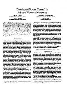
1.1 Example: Power Control in CDMA Networks Power control objectives are rather different when considering networks and not only links. In a CDMA system, each user is allocated a code, and the signal space is essentially spanned by the available orthogonal codes. The user’s data is recovered at the receiver by correlating the received signal with the allocated code. Due to channels, nonlinearities etc, this orthogonality is not preserved at the receivers. Instead, the code correlation (the scalar product) θ¯ij (t) ∈ [0, 1] between two codes of users i and j might be nonzero. Consider the simplistic uplink (mobile to base station) situation in Figure 1. Assume that the
2
In dB: γ(t) = p(t) + g(t) − I(t)
MS2 a) b)
MS1
Figure 1. Simplistic uplink and downlink situation with two mobiles connected to one base station to illustrate fundamental network limitations and objectives. The downlink (base station to mobile) situation is slightly different. All the signals from a base station to a specific mobile have passed through the same channel, and orthogonality can be assumed preserved. (This is not true in reality, mainly due to non-ideal receivers.) If the power of the signals from other cells and thermal noise at mobile 1 is denoted by ν¯1 (t), the SIR is given by γ¯1 (t) =
p¯1 (t)¯ gB1 , ν¯1 (t)
(3)
The downlink power is limited to P¯max = P¯D +P¯C , where P¯D is for user data and P¯C is for control signaling and pilot symbols used for channel estimation in the mobile. Hence P¯C ≥ p¯1 (t) + p¯2 (t) (vector addition due to different user codes). To fully utilize the hardware investment, the base station should use all the available power P¯D to provide services. The interesting question is how this power, and thus resulting service quality, should be shared between the users. Each connection-oriented service is typically regularly reassigned a reference SIR, γit (t) (note the switch to values in dB). Power control is used to maintain this SIR based on feedback of the error
ei (t) = γit (t) − γi (t). The feedback communication uses valuable bandwidth, and should be kept at a minimum. Let f (ei (t)) denote the feedback communication (essentially quantization). With pure integrating control, this yields pi (t + 1) = pi (t) + βf (ei (t))
among the users. An important distinction in Section 5.1 is therefore whether the network can accommodate all the users with associated quality requirements.
(4)
1.2 Aspects of Power Control Being subjective, the following list constitutes important aspects of power control:
2. SYSTEM MODEL Most quantities will be expressed both in linear and logarithmic scale (dB). Linear scale is indicated by the bar notation g¯(t).
Power Gain [dB]
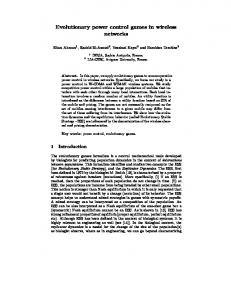
• Objectives. It is vital to clarify the aim 2.1 Power Gain of power control. As indicated in the example above, throughput maximation leads to By neglecting data symbol level effects, the comdifferent control strategies compared to fair munication channel can be seen as a time varyobjectives where all users experience roughly ing power gain made up of three components the same quality of service. g(t) = gp (t) + gs (t) + gm (t) as illustrated by • Centralized/decentralized control. CenFigure 2. The signal power drops with distance tralized power control is not practically d¯ to the transmitter, and the path loss is modtractable. As discussed in Section 5, it mainly ¯ Terrain variations eled as gp = K − α log10 (d). serves as theoretical performance bounds to cause diffraction phenomenons and this shadow the decentralized algorithms in Section 3. fading gs is modeled as AR(n)-filtered Gaussian • Feedback bandwidth. The feedback bandwhite noise (n is typically 1-2, (Sørensen, 1998)). width should be stated as the number of The multipath model considers scattering of radio available bits per second for feedback comwaves, yielding a rapidly varying gain gm (Sklar, munication. Then, this becomes a trade-off 1997). between error representation accuracy and feedback rate as discussed in Section 3.1 −80 gs • Power constraints. The transmission powgp −85 ers are constrained due to hardware limitations such as quantization and saturation, which is in focus in Sections 3.3PSfrag and 3.5. replacements −90 • Time delays. Measuring and control signal−95 ing take time, resulting in time delays in the distributed feedback loops. The time delays gm −100 are typically fixed due to standardized sig0 5 10 15 20 naling protocols, and are further treated in Travelled distance [m] Section 3.3 • Disturbance rejection. The controller’s Figure 2. The power gain g(t) is modeled as the ability to mitigate time varying power gains sum of three components: path loss gp (t), and measurement noise is an important pershadow fading gs (t) and multipath fading formance indicator further discussed in Secgm (t). Here this is illustrated when moving tion 3.3. from a reference point and away from the • Soft handover. One important coverage imtransmitter. proving feature in DS-CDMA systems it that a mobile can be connected to a multitude of base stations. This puts some specific re2.2 Wireless Networks quirements on power control which are briefly touched upon in Section 4.4. Consider a general network with m transmitters • Stability and convergence. Studying stausing the powers p¯i (t) and m connected receivers. bility and oscillatory behavior of the disFor generality, the base stations are seen as multitributed control loops as in section 3.4 is necple transmitters (downlink) and multiple receivers essary, but not sufficient. The cross-couplings (uplink). The signal between transmitter i and rebetween the loops also have to be considered. ceiver j is attenuated by the power gain g¯ij . Thus This is addressed in Section 5.2. the receiver connected to transmitter i will expe• Capacity and system load. As indicated rience a desired signal power C¯i (t) = p¯i (t)¯ gii (t) by the example above, the available radio and an interference from other connections plus resource is limited and have to be shared
noise I¯i (t). The signal-to-interference ratio (SIR) at receiver i can be defined by C¯i (t) g¯ii (t)¯ pi (t) γ¯i (t) = ¯ =P , (5) ¯ Ii (t) ¯ij (t)¯ pj (t) + ν¯i (t) j6=i θij g where θ¯ij is the normalized cross-correlation between the waveforms of user i and j, and ν¯i (t) is thermal noise. To keep the notation clear, we define θ¯ii = 1, and redefine the power gain to incorporate the cross-correlations: g¯ij := θ¯ij g¯ij . Depending on the receiver design, propagation conditions and the distance to the transmitter, the receiver is differently successful in utilizing the available desired signal power p¯i g¯ii . Assume that receiver i can utilize the fraction δ¯i (t) of the desired ¡ ¢ signal power. Then the remainder 1 − δ¯i (t) p¯i g¯ii acts as interference, denoted autointerference (Godlewski and Nuaymi, 1999). We will assume that the receiver efficiency changes slowly, and therefore can be considered constant. Hence, the SIR expression in Equation (5) transforms to γ ¯i (t) =
P
δ¯i g¯ii (t)¯ pi (t) ¡ ¢ . g ¯ (t)¯ p (t) + 1 − δ¯i p¯i (t)¯ gii (t) + ν¯i (t) ij j j6=i (6)
From now on, this quantity will be referred to as SIR. For efficient receivers, δ¯i = 1, and the expressions (5) and (6) are equal. In logarithmic scale, the SIR expression becomes γi (t) = pi (t) + δi + gii (t) − Ii (t).
(7)
2.3 Power Control Algorithms We adopt the loglinear power control model in (Blom et al., 1998; Dietrich et al., 1996) to embrace central power control approaches. The cascade control block diagram of a generic distributed SIR-based power control algorithm is depicted in Figure 3. The receiver computes the error ei as the difference between the reference SIR γit and SIR (measured, subject to measurement noise wi and possible filtered by the device Fi 3 ). The error is coded into power control commands ui by the device Ri , affected by command errors xi on the feedback channel and decoded on the transmitter side by Di . The control loop is subject to power update delays of np samples and measurement delays nm samples. Typically, np = 1 and nm . An outer loop adjusts the reference SIR to assure that the quality of service is maintained. Outer loop control is typically based on bit error rates (BER) and block error rate (BLER) (Olofsson et al., 1997; Wigard and Mogensen, 1996). 3
In practice, the desired signal power and the interference are typically filtered separately with filters Fg,i and FI,i .
3. DISTRIBUTED POWER CONTROL 3.1 Feedback Bandwidth The feedback signaling bandwidth is limited in real systems. Typically, the communication is restricted to a fixed number k of bits per second. The evident trade-off is between error representation accuracy and feedback command rate. A single bit error representation allow k feedback commands per second, while me bits error representation allow k/me commands per second. This comparison is further explored in (Gunnarsson, 2001). Different error representations are proposed, for example: single bit (the sign of the error) (Salmasi and Gilhousen, 1991), k-bit linear quantizer (Sim et al., 1998) and k-bit logarithmic quantizer (Li et al., 2001). All these corresponds to quantizers and decoders in the devices Ri and Di in Figure 3. Note also that the error representation is related to the command error rate on the feedback channel. 3.2 Power Control to Improve Link Performance Power control algorithms aiming at optimizing link performance mainly focus on link throughput and energy-effectiveness. One example (Goldsmith, 1997) actually meets the Shannon bound by transmitting more data when the channel is favorable (instead of using only little power to equalize SIR). Such strategies primarily considers information theoretical aspects of power control rather than network aspects. 3.3 Log-Linear Design Early work such as (Foschini and Miljanic, 1993) addresses the problem in linear scale based on iterative methods for eigenvector computations (Fadeev and Fadeeva, 1963). Thereby, it is closely related to the global aspects in Section 5. In logarithmic scale, this is the special case β = 1 of an integrating controller pi (t + 1) = pi (t) + βei (t)
(8)
The algorithm proposed in (Yates, 1995) controller above with an arbitrary β. A comparison to Figure 3 yields that this corresponds to Ri {ei (t)} = ei (t) (the exact error signal is asβ sumed), Di (q) = q−1 and no filtering. For reasons that will be evident later, the following interpretation is more natural when considering the academic example of perfect error representation: β , ui = pi , Di {pi (t−np )} = pi (t−np ). R(q) = q−1 (9)
xi (t)
Transmitter
Receiver QoSt
Outer Loop
γit (t)
ei (t)
Σ + −
γ ˆi (t)
Ri
ui (t)
q −np
Σ
Di
δi + gii (t) − Ii (t)
Environ.
pi (t − np )
Σ
wi (t)
Fi
q −nm
Σ
γi (t)
Decoding
Figure 3. Block diagram of the receiver-transmitter pair i when employing a general SIR-based power control algorithm. In operation, the controller result in a closed local loop. This has motivated the alternative linear designs of R(q) as PI-controllers and more general linear controllers in (Gunnarsson et al., 1999). For example, it provides optimally fast I and PI controllers when subject to time delays. Perfect error representation results in a linear distributed control loop with closed loop system Gll (q) and sensitivity S(q) given by Gll (q) =
q np +nm R(q) , S(q) = q np +nm + R(q) q np +nm + R(q) (10)
With the single bit power control command as in (Salmasi and Gilhousen, 1991), the integrating controller becomes pi (t + 1) = pi (t) + β sign (ei (t))
(11)
The transmitter power is constrained in practice, typically quantized and bounded from above and below. Grandhi et al. (1995) proposes an algorithm to deal with powers bounded from above. In log-linear scale it is given by pi (t + 1) = min {pmax , pi (t) + βei (t)}
(12)
This can be interpreted as one out of many possible anti-reset windup implementations for PI-controllers (˚ Astr¨om and Wittenmark, 1997), which thus can be employed to more general transmitter power constraints. The proposed power control algorithm for limited and quantized transmitter powers in (Wu and Bertsekas, 1999) is not linear and nor fully distributed, but is worth mentioning, due to its optimization approach. Time delays are critically limiting the closed-loop performance of any feedback system, and so also with power control. They therefore have to be considered in the design phase. The time delays are known and fixed, since the signaling and measurement procedures are standardized, and propagation delays are neglectable (except possibly in satellite communications). For example, the typical delay situation np = 1 and nm = 0 yields
γi (t) = pi (t − 1) + gii (t) − Ii (t)
(13)
Since the delays are exactly known, time delays can be compensated for using the Smith predictor (˚ Astr¨om and Wittenmark, 1997) as described in (Gunnarsson and Gustafsson, 2001b). Essentially, it is implemented as a measurement adjustment γ˜i (t) = γi (t) + pi (t) − pi (t − nm − np )
(14)
The actual power levels might not be available in the receiver, but rather the power control commands ui . These can, however, be used to recover the power level: pi = Di {ui }. With the Smith predictor, the closed loop system and the sensitivity becomes R(q) q np +nm (1 + R(q)) q np +nm S(q) = np +nm q (1 + R(q))
Gll (q) =
(15) (16)
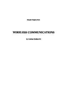
The local behavior of the controllers above is illustrated in simplistic simulations in Figure 4. We note that the disturbance rejection is satisfactory with most controllers. Furthermore, the benefits of using the Smith predictor are more emphasized with single-bit error representation. Roughly the same effect is obtained with linear design. This is in line with the results in (Kristiansson and Lennartsson, 1999). The Smith predictor might compensate for some dynamical effects, but the controllers still show delayed reactions to changes in the power gains. One approach to improve the reactions is to predict the power gain. Considering only shadow fading, the following model structure is relevant and fitted to data © ª C(q) es (t), Var e2s (t) = σe2 gs (t) = A(q)
Solve the Diophantine equation q m−1 C(q) = A(q)F (q) + G(q) for F (q) and G(q) yields the op-
γi (t) [dB]
ag replacementsc.
13
12
12
11
11
10
10
9
9
8
8
20
40
60
80
100
d.
γi (t) [dB]
14
13
12
12
11
11
10
10
9
9 20
40
60
80
t [s]
100
8
20
40
60
80
13 12 11 10
8 10
100
b. PSfrag replacements
20
30
40
50
60
70
80
90
100
20
30
40
50
60
70
80
90
100
14 13 12 11 10 9
20
40
60
80
100
8 10
t [s]
t [s]
Figure 4. Performance of different power control algorithms when subject to shadow fading and the typical delay situation np = 1, nm = 0. a. The PI-controller from pole placements design with (solid) and without (dashed) prefilter. b. The same controller at Ts = 0.015 (solid) and Ts = 0.05 (dashed). c. An optimized PI-controller (solid) and an I-controller with Smith predictor (dashed). d. The Icontroller with single-bit error representation (step-size 1 dB) with (dark gray) and without (light gray) Smith predictor. timal m-step predictor (˚ Astr¨om and Wittenmark, 1997) qG(q) gˆs (t + m|t) = gs (t) (17) C(q) Channel predictions are further studied based on linear model structures (Choel et al., 1999; Ericsson and Millnert, 1996) and nonlinear model structures (Ekman and Kubin, 1999; Tanskanen et al., 1998; Zhang and Li, 1997) When a disturbance model and an optimal predictor is available as above, the step to employ minimum variance control is slightly short (˚ Astr¨om and Wittenmark, 1997; Gunnarsson, 2000): R(q) =
14
9
14
13
8
a.
14
13
γi (t) [dB]
b.
14
γi (t) [dB]
a.
G(q) , q(q − 1)A(q)F (q)
(18)
where F (q) and G(q) are obtained from the Diophantine equation above, and attention is payed to include integral action into the controller. The performance using predictive and minimum variance controller is illustrated in Figure 5. Clearly, the error variance is significantly smaller than in Figure 4. As indicated in previous sections, it is not always justifiable to let a user disturb other connections significantly while aiming at a rather high SIR compared to the propagation conditions. In the proposed algorithm by Almgren et al. (1994), users aiming at using a high power are forced to use a lower SIR. The algorithm expressed in this framework is given by
Figure 5. Predictive control improve the performance by predicting the disturbances. a. PIcontroller with disturbance prediction (solid) and a minimum-variance controller (dashed). b. The single-bit error representation and Icontrol with the Smith predictor and disturbance prediction. R(q) =
β , q−β
(19)
which does not include integral action. The algorithm is further explored in (Yates et al., 1997). To keep the inner control loop simple and intuitive, an alternative is to implement such priorities in the outer control loop, see Section 3.5. In real systems, SIR is typically not readily available. One natural idea is to estimate SIR given available measurements. Approaches to do so in different systems are discussed in (Andersin et al., 1998; Blom et al., 1999; Ramakrishna et al., 1997). A different approach is to base the power control on the available measurements directly (Ulukus and Yates, 1998). There have also been proposals which aim at equalizing the received power at the connected base station (Anderlind, 1997; Salmasi and Gilhousen, 1991). The result by Ariyavisitakul (1994) concludes, however, that SIR based power control provides better control over the interference situation. All these algorithms are interpreted using the loglinear model. Uykan et al. (2000) proposes a PIcontroller in linear scale which is hard to interpret in the log-linear model. Whether it is more efficient to pursue power control in logarithmic scale than in linear scale is still unknown.
3.4 Analysis Local stability analysis is straightforward when the error representation is ideal, since the local control loop is all linear. E.g. root locus of the
poles to Gll (q) in (10) and (15) can be used to address local stability (Blom et al., 1998). It is easy to see that time delays make the choice of β in the I-controller crucial to ensure local stability. For example the choice β = 1 and already a time delay of one sample yield an unstable system, while it constitutes a dead-beat controller in the no delay situation. With the Smith predictor, this dead-beat behavior is essentially recovered. The single-bit error representation can be seen as relay feedback in a linear system. The oscillatory behavior can be approximated using discrete-time describing functions (Gunnarsson et al., 2001) yielding the oscillation period in samples as N = 2 + 4(np + nm ). Hence, the longer the delay, the more emphasized oscillatory behavior. This type of controller is also locally analyzed in (Song et al., 2001), where the relay is approximated by a constant and an additive disturbance yielding the same relay output variance. 3.5 Outer Loop SIR might be well correlated to perceived quality, but it is not possible to set a SIR reference offline, that result in a specific BER or BLER. Therefore, the inner control loop is operated in cascade with an outer loop, which adapts the SIR reference for a specific connection. Reliable communication can be seen as low BLER requirements, which in turn means that it is very hard to accurately estimate BLER. The errors appears rather seldom and it takes long time before the BLER estimate is stable. One implemented approach in several systems (Sampath et al., 1997) increases the SIR reference significantly when an erroneous block is discovered, and decreases the SIR reference when an error-free block is received. Niida et al. (2000) provides experimental results of outer loop power control using this method. One block comprises many bits. Therefore, it is easier to obtain a good BER estimate. Then the relation between BER and BLER can be utilized to predict BLER based on BER measurements (Kawai et al., 1999). Another outer loop control mechanism is to adapt the rate (Balachandran et al., 1999; Uvliden et al., 1998). In the uplink, rate adaption is supported by the mobile in WCDMA (3GPP, 2001, document 25.321). Essentially, the optional feature allows the mobile to automatically increase its data rate and its SIR reference when the propagation conditions are favorable and vice versa. 3.6 Downlink Issues As indicated by the introductory example, downlink power control objectives can be rather different and specific. The power control objectives
depend on the policies of the network operator, and can be differentiated in terms of service requirements, resource utilization, subscription conditions etc. Revisit the introductory example in Figure 1. Some natural policies are: • Aim at equal data rate (¯ γ1 (t) ≈ γ¯2 (t)). • Aim at equal power usage (¯ p1 (t) ≈ p¯2 (t)). • Use all power to transmit to the user with highest power gain (i.e. mobile 1 as indicated by the figure) to maximize throughput. • First use power to meet the quality of service requirements of users with more expensive subscriptions. Use the reminder to low-fare subscription users. Various downlink power control and resource sharing issues are brought up in (De Bernardi et al., 2000; Lu and Brodersen, 1999; Song and Holtzman, 1998; Vignali, 2001). Another problem is uneven traffic distributions that are not supported by the cell layout. In such a scenario, some cells might be overloaded, while others are under-utilized. The users select base stations based on measured pilot powers from the different base stations. By controling the pilot powers, the cells can be made larger or smaller. This is often referred to as cell breathing (Hwang et al., 1997).
4. STANDARDIZED POWER CONTROL ALGORITHMS Several power control algorithms are standardized by 3GPP to be used in WCDMA (3GPP, 2001, document 25.214). In GSM, the situation was different, since the mobile serves as slaves, using the power determined by the system. Therefore, power control is not standardized except control and measurement signaling (GSM).
4.1 Fixed-Step Power Control The power level is increased/decreased depending whether the measured SIR is below or above target SIR, and implemented as: Receiver : Transmitter :
ei (t) = γit (t) − γi (t)
(20a)
si (t) = sign (ei (t))
(20b)
pT P C,i (t) = ∆i si (t)
(20c)
pi (t + 1) = pi (t) + pT P C,i (t) (20d) where si (t) are denoted the TPC (transmitter power control) commands. This is the default choice both in the uplink and the downlink closed-loop power control. The uplink situation is slightly modified when the mobile is in soft handover. Then, the mobile receives power control
commands from every connected cell. To ensure that the power is adapted to the best cell, the mobile only increases the power if all commands are equal to +1, otherwise the power is decreased. This algorithm is equal to the single-bit error representation with pure integration in (11).
4.2 Uplink Alternatives This alternative algorithm is a different command decoding than above and is denoted ULAlt1. It makes it possible to emulate slower update rates, or to turn off uplink power control by transmitting an alternating series of TPC commands. In a 5-slot cycle (j = 1, . . . , 5), the power update pT P C,i (t) in (20c) is computed according to: 5 X ∆i si (j) = 5) (j = 5)&( j=1 5 X pT P C,i (t) = si (j) = −5) −∆ (j = 5)&( i j=1 0 otherwise (21) 4.3 Downlink Alternatives There are two downlink alternatives, both aiming at reducing the risk of using excessive powers. In the first one, here denoted by DLAlt1, the control commands are repeated over three consecutive slots. The second one, denoted DLAlt2, reduces the controllers ability to follow deep fades by limiting the power raise. As with the ULAlt1, the commands are decoded differently than in Section 4.1, described as an alternative to (20c):
pT P C,i (t) =
−∆i
∆i
si (t) < 0 (si (t) > 0)&(psum,i (t) + ∆i < δsum )
0
otherwise (22)
where psum,i (t) is the sum of the previous N power updates and N and δsum are configurable parameters.
this might lead to unwanted effects. The mobile algorithm of the TPC command combination is not standardized, and the problem is addressed in Grandell and Salonaho (2001). For downlink power control, the base stations adjusts its powers according to the received TPC command from the mobile. Due to feedback errors, these powers might drift from the ideal power levels. To compensate for this drift, a centralized power balancing is proposed in the standards, see 3GPP.
5. GLOBAL ANALYSIS For practical reasons, power control algorithms in cellular radio systems are implemented in a distributed fashion. However, the local loops are inter-connected via the interference between the loops, which affects the global dynamics as well as the capacity of the system. An important global issue is whether it is possible to accommodate all users with their service requirements. The power gains reflect the situation from the transmitters to the receivers, and the results are therefore applicable to both the uplink and the downlink. Sufficient conditions on global stability are derived, including the effect of time delays and general log-linear power control algorithms and filters. These conditions can be formulated as requirements on the local loops. The interesting conclusion is thus that global stability can be granted by proper design of the local loops.
5.1 Performance Upper Bounds and Feasibility The individual target SIR:s and the power gains are considered constant in the global level analysis, where the latter is motivated by an assumption that the inner loops perfectly meets the provided SIR reference, and thereby mitigates the fast channel variations. Note that values in linear scale are used in this section. δ¯i g¯ii p¯i ¢ ¡ P = γ¯it , ∀i (23) g¯ij p¯j + 1 − δ¯i p¯i g¯ii + ν¯i j6=i
Introduce the matrices 4.4 Soft Handover One corecentral feature in DS-CDMA systems is soft handover, where the mobile can connect to several base stations simultaneously. For best performance, the mobiles controls its power with respect to the signal from the base station with the most favorable propagation conditions. Intuitively, the mobile only increases the power if the TPC commands from all the base stations require it to do so. When command errors occur,
· ¸ ¯ij 4 g 4 t ¯ = [¯ ¯t = ), Z zij ] = Γ diag(¯ γ1t , . . . , γ¯m , g¯ii ¡ ¢ 4 ¯ = ∆ diag δ¯1 , . . . , δ¯m
and vectors
4
4
¯ = [¯ ¯ = [¯ p pi ] , η ηi ] =
·
¸ ν¯i . g¯ii
The network itself put restrictions on the achievable SIR’s, and there exists an upper limit on the balanced SIR (same SIR to every connection).
This is disclosed in the following theorem, neglecting auto-interference and assumes that the noise can be considered zero Theorem 1. (Zander, 1992). With probability one, there exists a unique maximum achievable SIR in the noiseless case ¯ ≥ 0 : γ¯i ≥ γ¯0 , ∀i}. γ¯ ∗ = max{¯ γ0 | ∃ p Furthermore, the maximum is given by 1 γ¯ ∗ = ¯ ∗ , λ −1
¯ ∗ is the greatest real eigenvalue of Z ¯ . where λ ¯ ∗ > 1 implies that γ¯ ∗ > 0. Moreover, Note that λ ¯ ∗ is the eigenvector of the optimal power vector p + ∗ ∗ ¯ λ (i.e. k¯ p for any k ∈ R constitute an optimal power vector.). The effects of auto-interference is considered in (Godlewski and Nuaymi, 1999) The requirements in Equation (23) can be vectorized to ³ ´ ¯ t (∆ ¯ −1 Z ¯ − E)¯ ¯ −1 η ¯=Γ ¯ , p p+∆ (24) where E is the identity matrix. Solvability of the equation above is related to feasibility of the related power control problem, defined as
Definition 2. (Feasibility). A set of target SIR:s ¯ t is said to be feasible with respect to a network Γ ¯ ∆ ¯ and η ¯ , if it is possible to described by Z, ¯ so that the requireassign transmitter powers p ments in Equation (24) ¡are met. Analogously, the ¢ ¯ η ¯ Γ ¯ t is said to be ¯ , ∆, power control problem Z, feasible under the same condition. Otherwise, the target SIR:s and the power control problem are said to be infeasible. The degree of feasibility is described by the feasibility margin, which is defined below. The concept has been adopted from Herdtner and Chong (2000), where similar proofs of similar and additional theorems covering related situations also are provided. Herdtner and Chong used the term feasibility index RI and omitted auto-interference. Definition 3. (Feasibility Margin). Given a power ¯ η ¯ Γ ¯ t ), the feasibility margin ¯ , ∆, control problem (Z, + ¯ Γm ∈ R is defined by © ª ¯ t is feasible ¯ m = sup x Γ ¯∈R : x ¯Γ A motivation for introducing the name feasibility margin is to stress the similarity to the stability margin of feedback loops. The following theorem captures the essentials regarding feasibility margins.
Theorem 4. (Feasibility Margin). Given a power ¯ η ¯ Γ ¯ t ), the feasibility mar¯ , ∆, control problem (Z, gin is obtained as ¯ m = 1/¯ Γ µ∗ where µ ¯∗ is
n o ¯ t (∆ ¯ −1 Z ¯ − E) . µ ¯∗ = max eig Γ
¯ m > 1, the power control problem Moreover, if Γ is feasible, and there exists an optimal power assignment, given by ³ ´−1 ¯ t (∆ ¯ −1 Z ¯ − E) ¯ −1 η ¯ t∆ ¯ = E−Γ ¯. p Γ PROOF. See (Gunnarsson, 2000; Gunnarsson and Gustafsson, 2001a). The power assignment above can of course be seen as a centralized strategy. However, since it requires full information about the network it is not plausible in practice, and the result mainly serves as a performance bound. The feasibility margin can also be related to the load of the system. When the feasibility margin is one, the system clearly is fully loaded (only possible when unlimited transmission powers are available). Conversely, when the feasibility margin is large, the load is low compared to a fully loaded system. Thus the following load definition is plausible. ¯r Definition 5. (Relative Load). The relative load L of a system is defined by ¯ r = 1 (= µ ¯∗ in Theorem 4). L ¯m Γ Feasibility of the power control problem is thus equal to a system load less than unity. For a more detailed capacity discussion, see (Hanly, 1999; Zhang and Chong, 2000), where receiver and code sequence effects also are considered. 5.2 Convergence and Global Stability As commented in Section 3.4, the integrating controller in (8) with β = 1 becomes unstable when subject to time delays. As concluded in the following theorem, global stability is regained by employing the Smith predictor. Theorem 6. The algorithm (8) and βi = 1 subject to a delay of n samples and employing the Smith ¯∞ predictor converges to a unique equilibrium p that meets the requirements in (23) with equality ¯ 0 . The convergence for any initial power vector p rate is n + 1 times slower compared to the algorithm (8) applied to a delayless power control problem.
PSfrag replacements PROOF. See (Gunnarsson, 2000; Gunnarsson and Gustafsson, 2001a).
FI (q)
∆cc ˜ (t) p
The WCDMA algorithm described in Section 4.1 with single-bit error representation never converges to a fixed point, as disclosed in Section 3.4. Instead, it converges to a region characterized by the following theorem. Theorem 7. If the power control problem is feasible, the algorithm without and with the Smith predictor (subject to a round-trip delay of totally nRT = 1 + np + nm samples, nRT = 1, 2, . . .) converges to a region where the SIR error for every connection is bounded (in dB) by Without Smith: With Smith:
|γit − γi (t)| ≤ 2nRT β
|γit − γi (t)| ≤ (nRT + 1)β
and β is the step size. The result also holds when subject to auto-interference. PROOF. The result without the Smith predictor is provided in (Herdtner and Chong, 2000), while the result with the Smith predictor is from (Gunnarsson, 2000; Gunnarsson and Gustafsson, 2001a). The global system can be seen as a diagonal system of local control loops, inter-connected by a static nonlinearity via the interference. By linearizing the interference around the equilibrium corresponding to the power vector that satisfies (24), this picture is simplified to a diagonal system with an unknown structured uncertainty. Full details are provided in (Gunnarsson, 2000), and the remainder of the section provides a sketched road-map to the result. The existence of such an equilibrium point is a consequence of the feasibility of the power control problem. 4
Introduce the MIMO system G(q) = Gll (q)E, where the closed local loop system Gll (q) is given by (10) and (15). With the equilibrium power ˜ (t), the linearized global system can deflection p be written as ˜ (t) = G(q)FI (q)∆cc p ˜ (t) + G(q)F g (q)˜ p g (t), (25) where ∆cc is the Jacobian of the interference with respect to the power vector. Figure 6 illustrates the corresponding block diagram of the global system (with a linear measurement filter). The infinity norm of the interference Jacobian is given by Lemma 8. The following relation holds for the matrix ∞-norm of the cross coupling matrix ∆cc ¶ µ v¯i k∆cc k∞ = max 1 − ¯t = δcc < 1 1≤i≤m Ii
˜ (t) g Fg (q)
P
G(q)
Figure 6. Block diagram of the global system, when approximating the interference by the corresponding linearization with respect to ˜ (t). the equilibrium deflection p The value of the norm δcc will be referred to as the degree of cross-coupling. The degree of cross-coupling δcc allows a natural interpretation. Essentially, it reflects the influence of the interference to the global system stability. Two cases are easily distinguished • δcc = 0. Corresponds to the case when the interference at every receiver is only noise, i.e. the local loops are operating independently. In such a situation, the local loop analysis in Section 3.4 is sufficient. • δcc = 1. Impossible in practice, since it corresponds to the case when the thermal noise is zero, or the interference at one receiver is infinite. However, in highly loaded interference limited systems, δcc is close to 1. The Small Gain Theorem is directly applicable to the block diagram in Figure 6 to address stability of the linearized system Theorem 9. Let Gll (q) be the stable closed-loop transfer function of the local loop. Then the global system in Figure 6 is stable if and only if the power control problem is feasible and any of the following properties is satisfied (i) supw |Gll (eiw )| ≤ 1/δF . (ii) supw |Gll (eiw )| < 1/(δcc δF ), where δF = sup |Fg (eiw )| w µ ¶ v¯i δcc = max 1 − ¯t 1≤i≤m Ii PROOF. See (Gunnarsson, 2000). We note that a highly loaded system is much harder to control (put narrower restrictions on local loop performance) than a slightly loaded system. For example rather aggressive strategies such as minimum-variance are only applicable in systems with little load to avoid violating the global stability.
6. CONCLUSIONS AND FUTURE WORK The area of power control in wireless networks is surveyed, and the power control algorithms are put into a control theory context to relate to the control nomenclature. With this common framework, it is natural to address critical properties such as stability and convergence. Still, many problems remains to be solved, primarily for downlink power control, where the objectives are more policy oriented and dependent on the network operator philosophy. Natural trade-offs are between fairness and throughput. The ambition with the extensive citation list is to provide, yet subjective, an overview of central proposals, and pointers to interesting open problems. 7. BIOGRAPHY Fredrik Gunnarsson received his PhD degree from Link¨opings universitet, Sweden 2000. Currently, he work on methods for power control field trial evaluation and with higher level radio resource management for WCDMA at Ericsson Research. He also holds a research position at Link¨opings universitet, and is responsible for the telecom projects within the competence center ISIS led by Prof. Lennart Ljung. Fredrik Gustafsson is professor of the chair in Communication Systems at Link¨opings universitet. His research interests include adaptive signal processing with telecom, avionic, and automotive applications. REFERENCES 3GPP. Technical specification group radio access network. Standard Document Series 3G TS 25, Release 1999, 2001. M. Almgren, H. Andersson, and K. Wallstedt. Power control in a cellular system. In Proc. IEEE Vehicular Technology Conference, Stockholm, Sweden, June 1994. E. Anderlind. Resource Allocation in Multi-Service Wireless Access Networks. PhD thesis, Radio Comm. Systems Lab., Royal Inst. Technology, Stockholm, Sweden, October 1997. M. Andersin, N.B. Mandayam, and D.Y. Yates. Subspace based estimation of the signal to interference ratio for TDMA cellular systems. Wireless Networks, 4(3), 1998. S. Ariyavisitakul. Signal and interference statistics of a CDMA system with feedback power control - part II. IEEE Transactions on Communications, 42(2/3/4), 1994. K. ˚ Astr¨ om and B. Wittenmark. Computer Controlled Systems – Theory and Design. Prentice-Hall, Englewood Cliffs, NJ, USA, third edition, 1997. K. Balachandran, S.R. Kadaba, and S. Nanda. Channel quality estimation and rate adaption for cellular mobile radio. IEEE Journal on Selected Areas in Communications, 17(7), 1999. J. Blom, F. Gunnarsson, and F. Gustafsson. Constrained power control subject to time delays. In Proc. International Conference on Telecommunications, Chalkidiki, Greece, June 1998.
J. Blom, F. Gunnarsson, and F. Gustafsson. Estimation in cellular radio systems. In Proc. IEEE International Conference on Acoustics, Speech, and Signal Processing., Phoenix, AZ, USA., March 1999. S. Choel, T. Chulajata, H. M. Kwon, B.-J. Koh, and S.C. Hong. Linear prediction at base station for closed loop power control. In Proc. IEEE Vehicular Technology Conference, Houston, TX, USA, May 1999. R. De Bernardi, D. Imbeni, L. Vignali, and M Karlsson. Load control strategies for mixed services in WCDMA. In Proc. IEEE Vehicular Technology Conference, Tokyo, Japan, May 2000. P. Dietrich, R.R. Rao, A. Chockalingam, and L. Milstein. A log-linear closed loop power control model. In Proc. IEEE Vehicular Technology Conference, Atlanta, GA, USA, April 1996. T. Ekman and G. Kubin. Nonlinear prediction of mobile radio channels: measurements and MARS model designs. In Proc. IEEE International Conference on Acoustics, Speech, and Signal Processing, Phoenix, AZ, USA, March 1999. A. Ericsson and M. Millnert. Fast power control to counteract rayleigh fading in cellular radio systems. In Proc. RVK, Lule˚ a, Sweden, 1996. D.K. Fadeev and V.N. Fadeeva. Computational Methods of Linear Algebra. W.H. Freeman, San Fransisco, CA ,USA, 1963. G.J. Foschini and Z. Miljanic. A simple distributed autonomus power control algorithm and its convergence. IEEE Transactions on Vehicular Technology, 42(4), 1993. P. Godlewski and L. Nuaymi. Auto-interference analysis in cellular systems. In Proc. IEEE Vehicular Technology Conference, Houston, TX, USA, May 1999. A.J. Goldsmith. The capacity of downlink fading channels with variable rate and power. IEEE Transactions on Vehicular Technology, 46(3), 1997. J. Grandell and O. Salonaho. Closed-loop power control algorithms in soft handover for WCDMA systems. In Proc. IEEE International Conference on Communications, Helsinki, Finland, June 2001. S.A. Grandhi, J. Zander, and R. Yates. Constrained power control. Wireless Personal Communications, 2(1), 1995. GSM. Radio Subsystem Link Control. GSM Recommendations 05.08, ETSI, 1994. F. Gunnarsson. Power Control in Cellular Radio System: Analysis, Design and Estimation. PhD thesis, Link¨ opings universitet, Link¨ oping, Sweden, April 2000. F. Gunnarsson. Fundamental limitations of power control in WCDMA. In Proc. IEEE Vehicular Technology Conference, Atlantic City, NJ, USA, Oct 2001. F. Gunnarsson and F. Gustafsson. Convergence of some power control algorithms with time delay compensation. Submitted to IEEE Transactions on Wireless Communications, 2001a. F. Gunnarsson and F. Gustafsson. Time delay compensation in power controlled cellular radio systems. IEEE Communications Letters, 5(7), Jul 2001b. F. Gunnarsson, F. Gustafsson, and J. Blom. Pole placement design of power control algorithms. In Proc. IEEE Vehicular Technology Conference, Houston, TX, USA, May 1999. F. Gunnarsson, F. Gustafsson, and J. Blom. Dynamical effects of time delays and time delay compensation in power controlled DS-CDMA. IEEE Journal on Selected Areas in Communications, 19(1), Jan 2001. S. Hanly and D.-N. Tse. Power control and capacity of spread spectrum wireless networks. Automatica, 35(12), 1999. S. V. Hanly. Congestion measures in DS-CDMA. IEEE Transactions on Communications, 47(3), 1999.
J.D. Herdtner and E.K.P. Chong. Analysis of a class of distributed asynchronous power control algorithms for cellular wireless systems. IEEE Journal on Selected Areas in Communications, 18(3), Mar 2000. H. Holma and A. Toskala, editors. WCDMA for UMTS. Radio Access for Third Generation Mobile Communications. Wiley, New York, NY, USA, 2000. S.-H. Hwang, S.-L. Kim, H.-S. Oh, C.-E. Kang, and J.-Y Son. Soft handoff algorithm with variable thresholds in CDMA cellular systems. IEE Electronics Letters, 33 (19), 1997. H. Kawai, H. Suda, and F. Adachi. Outer-loop control of target SIR for fast transmit power control in turbocoded W-CDMA mobile radio. IEE Electronics Letters, 35(9), 1999. B. Kristiansson and B. Lennartsson. Optimal PID controllers including roll off and Schmidt predictor structure. In Proc. IFAC World Congress, Beijing, P. R. China, July 1999. P. R. Kumar. New technological vistas for systems and control: The example of wireless networks. IEEE Control Systems Magazine, 21(1), 2001. W. Li, V.K. Dubey, and C.L. Law. A new generic multistep power control algorithm for the LEO satellite channel with high dynamics. To appear in IEEE Communications Letters, 2001. Y. Lu and R.W. Brodersen. Integrating power control, error correcting coding, and scheduling for a CDMA downlink system. IEEE Journal on Selected Areas in Communications, 17(5), May 1999. S. Niida, T. Suzuki, and Y. Takeuchi. Experimental results of outer-loop transmission power control using wideband-CDMA for IMT-2000. In Proc. IEEE Vehicular Technology Conference, Tokyo, Japan, May 2000. H. Olofsson, M. Almgren, C. Johansson, M. H¨ oo ¨k, and F. Kronestedt. Improved interface between link level and system level simulations applied to GSM. In Proc. IEEE International Conference on Universal Personal Communications, San Diego, CA, USA, October 1997. D. Ramakrishna, N.B. Mandayam, and R.D. Yates. Subspace based estimation of the signal to interference ratio for CDMA cellular systems. In Proc. IEEE Vehicular Technology Conference, Phoenix, AZ, USA, May 1997. Z. Rosberg and J. Zander. Toward a framework for power control in cellular systems. Wireless Networks, 4(3), 1998. A. Salmasi and S. Gilhousen. On the system design aspects of code division multiple access (CDMA) applied to digital cellular and personal communications networks. In Proc. IEEE Vehicular Technology Conference, New York, NY, USA, May 1991. A. Sampath, P.S. Kumar, and Holtzman J.M. On setting reverse link target SIR in a CDMA system. In Proc. IEEE Vehicular Technology Conference, Phoenix, AZ, USA, May 1997. C.E. Shannon. The zero error capacity of a noisy channel. IRE Transactions On Information Theory, 2, 1956. M.L. Sim, E. Gunawan, C.B. Soh, and B.H. Soong. Characteristics of closed loop power control algorithms for a cellular DS/CDMA system. IEE Proceedings - Communications, 147(5), October 1998. B. Sklar. Rayleigh fading channels in mobile digital communication systems. IEEE Communications Magazine, 35(7), 1997. L. Song and J.M. Holtzman. CDMA dynamic downlink power control. In Proc. IEEE Vehicular Technology Conference, Ottawa, Canada, May 1998. L. Song, N.B. Mandayam, and Z. Gajic. Analysis of an up/down power control algorithm for the CDMA reverse link under fading. IEEE Journal on Selected Areas in Communications, Wireless Communications Series, 19 (2), 2001.
T.B. Sørensen. Correlation model for slow fading in a small urban macro cell. In Proc. IEEE Personal, Indoor and Mobile Radio Communications, Boston, MA, USA, September 1998. J. Tanskanen, J. Mattila, M. Hall, T. Korhonen, and S. Ovaska. Predictive estimators in CDMA closed loop power control. In Proc. IEEE Vehicular Technology Conference, Ottawa, Canada, May 1998. S. Ulukus and R. Yates. Stochastic power control for cellular radio systems. IEEE Transactions on Communications, 46(6), 1998. A. Uvliden, S. Bruhn, and R. Hagen. Adaptive multi-rate. A speech service adapted to cellular radio network quality. In Proc. Asilomar Conference on Signals, Systems & Computers, Pacific Grove, CA, USA, November 1998. Z. Uykan, R. J¨ antti, and H.N. Koivo. A pi-power control algorithm for cellular radio systems. In Proc. IEEE International Symposium on Spread Spectrum Techniques and Applications, New Jersey, NJ, USA, September 2000. L. Vignali. Admission control for mixed services in downlink WCDMAin different propagation environments. In Proc. IEEE Personal, Indoor and Mobile Radio Communications, San Diego, CA, USA, October 2001. J. Wigard and P. Mogensen. A simple mapping from C/I to FER and BER for a GSM type of air-interface. In Proc. IEEE Personal, Indoor and Mobile Radio Communications, Taipei, Taiwan, October 1996. C.C. Wu and D.P. Bertsekas. Distributed power control algorithms for wireless networks. In Proc. IEEE Conference on Decision and Control, Phoentix, AZ, USA, Dec 1999. R.D. Yates. A framework for uplink power control in cellular radio systems. IEEE Journal on Selected Areas in Communications, 13(7), September 1995. R.D. Yates, S. Gupta, C. Rose, and S. Sohn. Soft dropping power control. In Proc. IEEE Vehicular Technology Conference, Phoenix, AZ, USA, May 1997. J. Zander. Performance of optimum transmitter power control in cellular radio systems. IEEE Transactions on Vehicular Technology, 41(1), February 1992. J. Zander. Radio resource management in future wireless networks - requirements and limitations. IEEE Communications Magazine, 5(8), August 1997. J. Zhang and E.K.P. Chong. CDMA systems in fading channels: admissibility, network capacity, and power control. IEEE Transactions on Information Theory, 46 (3), 2000. Y. Zhang and D. Li. Power control based on adaptive prediction in the CDMA/TDD system. In Proc. IEEE International Conference on Universal Personal Communications, San Diego, CA, USA, October 1997.