interchangably. For degree, we will specify with. ° symbol as in common practice. whose sectors can collectively cover the whole 360. ⦠space. We assume the ...
Power-Efficient Broadcast Routing in Adhoc Networks Using Directional Antennas: Technology Dependence and Convergence Issues Intae Kang, Radha Poovendran and Richard Ladner Department of Electrical Engineering, University of Washington, Seattle, WA. 98195-2500 email: {kangit,radha,ladner}@ee.washington.edu
Abstract— We investigate the power-efficient broadcast routing problem using directional antennas. Our main interest is in the case when antenna beamwidth becomes very small. We consider asymptotic convergence properties of previously known broadcast routing algorithms and compare them with asymptotically optimal structures. Algorithms and techniques to reduce total transmit power using directional antennas—new and old—are introduced and summarized. We also present a dynamic programming solution to optimal beam assignment problem in multi-beam adaptive antennas. Extensive perfomance comparison results are also provided. Index Terms— Mathematical programming, optimization, broadcast, power efficient, routing algorithm, adhoc network, directional antenna.
I. I NTRODUCTION The idea of using directional antenna in wireless communications is not new. It has been already extensively used in base stations of cellular networks for frequency reuse, to reduce interference, and to increase the capacity of allowable users within a cell [1]. However, the application of directional or smart antennas 1 to wireless adhoc or sensor networks to reduce the transmit power of each node and hence to achieve power-efficiency in routing problem is relatively new. We consider all types of directional antenna systems of interest in this paper including switched beam or electronically steerable antenna systems [2]. Both wireless adhoc and cellular networks are known to be interference-limited [1], [3]. As a way to breakthrough in capacity limit proven in [3] for omnidirectional case, the use of directional antennas has begun to draw a lot of attention recently. The potential benefits of using directional antennas include range extension, better spatial reuse, multipath diversity, interference suppression, capacity increase, and data rate increase [4]. 1 Smart antenna is also known as phased array, adaptive array, software radio antenna, intellegent antenna etc.
Therefore, if done correctly, networking with directional antennas has great potential to provide significant enhancement over the one with omnidirectional antennas in capacity, power consumption, and network lifetime. Minimum power broadcast routing is still at the early stage of development. While several broadcast/multicast routing protocols have been proposed [5], they do not consider energy consumption in the design parameters. Publication of broadcast incremental power (BIP) algorithm by Wieselthier et al. [6] brought significant attention to this problem among the research community. In this paper, we address power-efficient broadcast routing problems using directional antennas. Our contributions are: (i) present power reduction techniques for different classes of antennas, (ii) investigate the asymptotic convergence properties of algorithms, and (iii) demonstrate that various assumptions on the directional antennas, which can be considered as being dependent on the development stage of antenna technology, can heavily affect the resulting routing structures. The remainder of this paper is organized as follows: In the next section, we briefly review the most relevant previous work. In Section III, a brief background on antenna model is provided. In Section IV, we present and summarize various power-efficient algorithms and techniques. In Section V, we discuss asymptotic behavior of algorithms and asymptotic optimal structures are introduced. Section VI summarizes our simulation results and Section VII presents conclusions and future work. II. R ELATED W ORK Excellent general overview and surveys on smart antennas can be found in [2], [4], [7]–[9]. Especially, Ramanathan’s work [2] deals with several issues of using smart antenna for adhoc networks, and argues that there are many imminent possible practical usages of smart antennas for adhoc networks even at a higher cost. Most of the work in ad hoc networking with directional antenna have been concentrated on medium access
control (MAC) [10]–[14]. Other interesting topics include topology control problem with directional antennas [15], [16] and capacity problems [3], [17], [18]. Energy efficient unicast routing with directional antennas was first introduced in [19]. In [20], two simple protocols to reduce control overhead by local directional flooding technique were proposed. [21] discusses modification to DSR [22] for use with directional antennas. Most closely related work to this paper includes [23]–[25]. In [23], Wieselthier et al. first considered adaptation of directional antennas to the well-known Broadcast Incremental Power (BIP) algorithm, which was originally developed for omnidirectional antennas. Two algorithms called Reduced Beam BIP (RB-BIP) and Directional BIP (D-BIP) were introduced in [23]. In [23], using adaptive array antennas (a class of smart antenna) is implicitly assumed, because RB-BIP or DBIP algorithms require an unlimited number of antenna patterns and no assumption is made on the sectorization of beamwidth. RB-BIP algorithm is essentially same as BIP except that, after the BIP tree is constructed, the beamwidth of antenna is reduced to fit minimum possible angle to cover all child nodes of each node. On the other hand, D-BIP algorithm in [23] utilizes incremental power—additional power required to reach another node in the network—in the core of the algorithm while building a routing tree. A natural extension to BIP algorithm utilizing conventional sectored antenna was presented in [24]. We will conveniently call this algorithm Sectored BIP (S-BIP). In S-BIP, minimum incremental power is calculated persector basis, and the transmit power level is increased only for the single sector with minimum incremental power. Although the focus in [24] is limited to traditional sectored antennas, arguments in [24] are directly applicable to switched beam antennas. This reconfirmed that the incremental power is a good choice for a decision metric at each greedy decision process, which is applicable to all classes of antennas. In [25], we proposed a power-efficient broadcast routing algorithm which can be used along with switched beam antennas to show that broadcast efficiency is a viable decision metric. In addition, asymptotic behavior, which is the main contribution of this paper, was preluded. III. A NTENNA M ODEL Many previous literature assume lots of different models of directional antennas. Different, sometimes inaccurate, assumptions make valid comparison difficult and can possibly lead to inconsistent results. Also in
designing an algorithm, optimal structure can be different depending on the used assumptions—one example is D-BIP algorithm [23] which will be discussed later in a greater detail in Section V-E. Therefore, a clear description of assumptions on antennas used are crucial. First, we introduce the class of antennas and later classify what assumptions are used for each type. A. Classification of Directional Antennas Directional antennas can be categorized at the highest level as conventional directed antennas (e.g., Yagi-Uda, helical, horn, reflector, patch antennas, etc.) and electronically steerable or smart antenna systems. A smart antenna is an antenna array system aided by smart DSP and control algorithms designed to adapt to different signal environment. An antenna array is a spatial geometric construction of antenna elements (e.g., linear, circular or planar, etc.) whose outputs are combined, selected, or weighted to enhance wireless system performance [26]. Main benefits of smart antenna are to improve the wireless system performance through [27]: (i) beamforming, (ii) space-time adaptive processing (STAP), and (iii) diversity processing. Smart antennas can be generally categorized as the following types [2], [7], [9]: 1) Switched Beam Antenna (SB): Antenna beam patterns are pre-defined. Weights for antenna elements which produce the desired beam pattern can be locally saved in memory and instantaneously switched. 2) Adaptive Array Antenna (AA): With this antenna type, by maximizing the output signal-to-interferenceplus-noise ratio (SINR) or minimizing the mean squared error (MMSE) using a training sequence, not only the beamforming is made so that the main beams (lobes) is directed to desired directions (boresight direction), but also interferences can be actively cancelled by null steering. If combining weights for elements are done to maximize the signal-to-noise ratio (SNR) and null steering capability is not assumed, then it is commonly called a phased array (PA). The main lobe can still be directed to any direction of signal-of-interest. B. Models for Antenna Radiation Pattern Radiation pattern of an antenna is angular dependence of beam power measured at the same (far-field) distance. An isotropic antenna has a spherical pattern due to an ideal point source located at the center radiating equally in all directions. An omnidirectional antenna has a constant (circular) radiation pattern in a plane, say, horizontal plane. A directional antenna has specific directions where energy is concentrated [26].
The (power) gain G (θ, φ) of an antenna is the ratio of radiation intensity to average intensity over all directions. If no direction is specified, the gain usually means the maximum gain value over all directions. Due to the reciprocity theorem, all the gain and radiation pattern characteristics are known to be same for both transmission and reception [26], [27]. In adhoc networking community, two simplistic models for gain and antenna patterns are popularly used: • Flat-top radiation pattern—This corresponds to an idealized angular response such that the gain is constant within the beamwidth and has no side lobes [23]. In 3D, an antenna beam (lobe) has the shape of a slice of pie. In this model, for a beam with beamwidth θ in azimuth, the gain is defined as � � 2π G= where θ ≥ θmin , (1) θ where θmin is the minimum achievable beamwidth determined by array length (aperture size) and wavelength, which is basically a technology limiting factor. • Cone+Sphere radiation pattern—This model was proposed in [2] and used in [13], [21] to account for the effects of sidelobes. Note that within the cone, the gain value is still constant. For details, readers are referred to [2]. In practice, the gain is a function of elevation and azimuth beamwidth, and usually approximated with the following formula: [27] G≈η
41000 , · φ◦HP
◦ θHP
(2)
◦ where θHP and φ◦HP represent the half-power 2 beamwidths in elevation and azimuth angles in degrees, and η denotes the radiation efficiency 0 ≤ η ≤ 1. The Cone+Sphere model in [2] assumed granularity in beamwidth as multiples of 10 degree. Because we require arbitrary beamwidth in our derivation and for easy comparison with earlier work [23]–[25], we will use the flat-top radiation pattern in this paper. In general, it is known that current technology can support up to 5◦ ∼10◦ beamwidth [14]. Analysis with other complicated radiation patterns is left as our future work.
C. Assumptions on Antenna Systems For the rest of this paper, we refer a sectored antenna to denote either a conventional sectored or SB antenna
whose sectors can collectively cover the whole 360 ◦ space. We assume the following regardless of antenna types: (i) All input power to the antenna is converted to radiated power e.g., η = 1 in (2). (ii) Antennas cannot transmit and receive at the same time. 1) Sectored Antenna: By assuming the flat-top radiation pattern, in case of sectored antennas, we inherently assume ideally sectorized system with no inter-sector interference. Furthermore, three sector alignment scenarios are possible: (i) All antennas are aligned to a specific direction (e.g., north) by a magnetic needle [21] within each antenna and m-th sector of each antenna covers a two dimensional plane over an angular region [(m − 2π 1) 2π M , m M ), (ii) randomly oriented with angular region 2π [(m−1) 2π M +θi , m M +θi ), where θi is a uniform random variable in [0, 2π] for each node i or (iii) optimally oriented by some optimization criteria. Antennas can be re-oriented by mechanical or MEMS aided rotation or electronically steered in case of switched beam antennas [26]. For simplicity, we will consider only the first scenario. 2) Adaptive Array Antenna: An adaptive array which can form multiple main beams/lobes is called a multibeam adaptive array (MBAA) [14]; otherwise, if it can form only a single beam, we will call it SBAA. With a multiple beamforming network (combiner) within a transceiver, a node can either simultaneously transmit or receive multiple traffic. This is known as space-division multiple access (SDMA) [27]. With an (M + 1)-element array, it is possible to specify M1 directions of desired signals (beamforming) and place M 2 nulls in the direction of unwanted interferences (null steering) such that M1 + M2 = M . This flexibility of an (M + 1)-element array to be able to fix the pattern at M places is known as the degree of freedom of the array [4], [9]. In broadcast or multicast routing, same messages need to be sent to multiple destinations. Using directional antenna, this can be achieved with multiple unicasts with SBAA or a single multicast with MBAA. Note that in multiple unicasts with SBAA case, it requires more delay to contact every child node and multiple processing to shift the beam, which require simple computations. On the other hand, multi-beamforming with MBAA requires more complex computations. Therefore, on average, we assume the amount of power consumption is same in both cases. 3 Consequently, we can use the existing antenna gain models.
2
As a unit for the beamwidth, we will use radian and degree interchangably. For degree, we will specify with ◦ symbol as in common practice.
3 This may not be true with real antennas because of the effects of sidelobes. But this is out of scope of this paper.
D. Transmission and Reception Modes
IV. P OWER -E FFICIENT B ROADCAST ROUTING
Due to path loss, the received power P r (d) at d distance apart from a node transmitting with transmit power Pt should be larger than receiver sensitivity threshold Ω for correct reception [1], [2]: Pr (d) =
Pt Gt Gr dα
�
λ 4π
�2
≥ Ω,
(3)
where Gt and Gr represent transmitter and receiver gains, respectively, λ is the wavelength, and α is the path loss (attenuation) factor that �satisfies �2 2 ≤ α ≤ 4. For notational simplicity, we set Ω 4π = 1 so that the λ minimum required transmit power for correct reception at a node d distance apart can be expressed as −1 α Pt (d) = G−1 t Gr d .
(4)
Therefore, the larger the gain is, the smaller the required transmit power. Let’s assume every antenna has two transmission (TX) and reception (RX) modes: omnidirectional and directional. We will put a prefix o-/d- to indicate the modes. If a receiver listens in d-RX mode, due to reciprocity theorem, the same gain as d-TX mode can be applied and hence the required transmit power can be further reduced, i.e., dα /G vs. dα /G2 assuming Gt = Gr = G. In d-TX/o-RX mode, while receivers are more susceptible to interferences, transmitters do not cause much interference to other nodes. In o-TX/d-RX, transmitters induce lots of interferences to other nodes, but because of directed listening, receivers are less affected. Hence, we assume the performance of d-TX/o-RX and o-TX/dRX is same and, in fact, (4) do not differentiate these. 4 Depending on the directivity of TX or RX mode, neighbor discovery and scheduling becomes a challenging problem. For example, with d-TX/d-RX mode, it has the potential to increase the gain to G 2 , but scheduling antenna beams to face each other at the same time becomes a challenging problem [10], [14]. Also, with increased range at the same power, new links can be discovered with directional modes, which was not possible with omnidirectional mode. In power-efficient broadcast routing problem, the gain in antennas is usually used to reduce the transmit power, not to increase the range. Hence, we do not require the use of newly discovered links. We assume that all links are discovered through o-TX/o-RX mode and actual broadcast can be done in directional modes. 4 In reality, however, there are subtleties such as transmitter diversity [12], [27] which make them different.
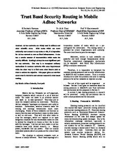
We have observed from previous research that powerefficient algorithm design can bring up to 15∼20% reduction in total transmit power over minimum weight spanning tree (MST) [6], [28]. The achievable gain by using smart antennas is much larger compared to what power-efficient algorithms using omnidirectional antennas can provide. Once smart antennas are used, whichever algorithm we use for broadcast routing, it is likely to improve power-efficiency due to large antenna gain. However, because battery energy is such a precious resource in wireless adhoc networks, it is still favorable to have power-efficient algorithms. A. Power Reduction Techniques In this section, we present three approaches to exploit beamforming capability of directional antennas in conjunction with algorithms for omnidirectional antennas. First approach is due to [23] and the following two are our own contributions. 1) Beam Angle Reduction (RBA) with Single Beam Adaptive Arrays: This technique was introduced in [23] to explain RB-BIP algorithm. It assumes that a single main lobe can be directed to any desired direction with arbitrary beamwidth as long as it is larger than minimum beamwidth θmin . Thus, this technique is suitable for PA or SBAA antennas. Also, flat-top antenna pattern and d-TX/o-RX operations were assumed. Clearly, this technique is not limited to BIP but is extensible to any tree construction algorithm. We apply this to MST, BIP [6], EWMA [28], and GPBE [29] algorithms. One example of this technique is presented in Fig. 1(b). 2) Beam Power Reduction (RBP) with Switched Beam Antennas: In case every node is equipped with a SB antenna, we can perform a conceptually similar operation as above. As mentioned before, we assume sector antennas are aligned to a common direction. Once a tree is determined, a SB antenna is imposed on top of every node. In individual sectors where there is no child node, no transmit power is assigned. If there exists at least one child node, nonzero transmit power is assigned such that all child nodes can be covered with minimum possible power. We don’t need to consider beamwidth because it is inherently determined by sectored antennas. In fact, it is possible to further reduce the transmit power of each node by rotating the sector of each node by a proper angle. However, on average, the performance should be similar and we do not consider this further. We assume that the beamwidth of each sector can be as small as the minimum beamwidth θmin in RBA case. Fig. 1(c) shows an example of RBP operation on trees.
EWMA: totalpower=403103.388 lifetime=119.3405
(a)
ο
RBA−EWMA, θmin = 30 , Ptx(T) = 161643.2409
RBP−EWMA, Sector = 12, P (T) = 122636.2555 tx
(b)
(c)
ο
OBR−EWMA, θmin = 30 , Ptx(T) = 94010.4729
(d)
Fig. 1. Illustration of power reduction techniques. N = 100 nodes are randomly distributed over 1x1 km2 region. Node locations and assigned beam range and shapes are shown. (α = 2) (a) original EWMA tree (b) reduced beam angle RBA-EWMA (c) reduced beam power RBP-EWMA (d) optimal beam reduction OBR-EWMA.
3) Optimal Beam Reduction (OBR) with Multi-Beam Adaptive Arrays: As mentioned earlier, MBAA antennas with (M + 1)-elements can support up to M main lobes and null steering. Because we do not require null steering in broadcast routing, let’s assume all degrees of freedom are dedicated to beamforming M main lobes. With added flexibility of MBAA, there should be a better way to assign the beamwidth and range of each lobe. Given a tree structure and a constraint on the number of beams M , what is the optimal beam assignment so that the total transmit power is minimized? Note that this problem is different from the minimum power broadcast problem which has been proven to be NP-hard [28] in that a tree structure is already determined. Thus, the total transmit power can be minimized by minimizing the transmit power of each node. We can solve this problem with a dynamic programming method.
Fig. 2. Illustration of dynamic programming setup for optimal beam reduction.
Dynamic Programming Solution to Optimal Beam Assignment Problem Let a node s has n child nodes and label each child node sorted in order by an angle from the x-axis as {1, 2, . . . , n}. Let θmin denote minimum beamwidth. From a reference starting line (see Fig. 2), angles are measured and the corresponding angle is {θ1 , θ2 , . . . , θn }, where θ1 = 0. The distances to the
parent node s are {d1 , d2 , . . . , dn }. Note that the values of θi and di for 1 ≤ i ≤ n are dependent on the position of the starting line. First, let’s define Ci,j as � � minimum cost of covering θi to θj Ci,j = (5) with a single beam � α α � = max {(θj − θi ), θmin } · max di , di+1 , . . . , d2j and find values for 1 ≤ i ≤ j ≤ n. Then, define B i,k as � � minimum cost of covering θi to θn Bi,k = with less than k beams =
min {Bi,k−1 , Bl+1,k−1 + Ci,l }
i≤l≤n−1
(6)
where Bi,1 = Ci,n . After initializing Bi,1 for 1 ≤ i ≤ n, we can find Bi,k for 2 ≤ k ≤ M and 1 ≤ i ≤ n − 1. This operation is repeated by letting the starting line start at each angle of node 1 through n. Then, the optimal solution with minimum transmit power is given by the minimum value �of B � 1,M for all starting lines. Finding 2 time complexity and finding [B ] [Ci,j ] requires O n i,k � � requires O n2 k time complexity. Because this operation is repeated n times for all starting lines, we get an optimal solution to this problem with time complexity � � O n3 M . Recall that this is only for a single node and hence this algorithm should be applied to every node in the� network. � Therefore, this problem can be solved in O n3 N M time, where n denotes the maximum node degree. Note that with M = 1, OBR reduces to RBA. B. Algorithms Adaptive to Directional Antennas Currently, there are not many algorithms for powerefficient broadcast routing tree that utilize the beamforming capability of directional antennas. The S-BIP [24], D-
BIP [23] and S-GPBE [25] are the algorithms we know of natively designed for directional antennas. In addition to these, other algorithms based on MST for SB or AA antennas are possible. Note that MST can be used equally well with directional antennas— assuming Prim’s algorithm, the decision made at each step is to choose the nearest node which has not been included in the current connected component. Whether SB or AA antennas are used, this decision does not change and hence the resulting link structure is same. The final structure of S-MST and D-MST will be identical to RBP-MST and OBR-MST, respectively. The only difference is that beam assignment is done on the fly while constructing a MST tree. V. A SYMPTOTIC B EHAVIOR Different assumptions on directional antennas can lead to different optimal structures. In general, it is hard or impossible to identify the optimal structure. However, asymptotic optimal solutions in different scenario can be easily identified by first looking at asymptotic behavior of decision space. In this section, we investigate the convergence properties when the path loss factor α becomes large or beamwidth θ min becomes narrower and corresponding optimal structures are investigated later.
the nodes are defined as d 1 = The distances between SA , d2 = SB , and d12 = AB , and the angle ∠ASB = θ . To broadcast from node S , there are four exhaustive cases: (S → B → A), (S → A → B), (S → {A, B}), (S → A, S → B). This is illustrated in order in Fig. 3, where each link and transmit range is shown. In the first two cases, node B and A relay the traffic for node S to reach the other node. We will call this decision as multihop M H B and M HA , respectively. The subscripts denote the relay node. In the third case, by a single transmission to node A, node B can get the message, which we will call broadcast advantage BA following [6]. Fourth example corresponds to the case when source S transmits the message to node A and node B with two unicast transmissions, which we will call 2U . Depending on the location of node B , we determine which decision requires minimum total transmit power and mark the position as one of the four decision choices {M HB , M HA , BA, 2U } .
A. Optimal Decision Space with Omnidirectional Antenna It has been observed by others (see e.g., [28]) that when the path loss factor α increases, both BIP and EWMA algorithms converge to MST. In essence, the main reason is that the cost of choosing longer links becomes more expensive as α becomes large. Hence, both algorithms tend to choose links with smaller transmit power, which is in principle the behavior of MST. Instead of general verbal explanation, if there is a way to visualize the effect, it will be helpful to understand this behavior. For this purpose, we introduce a decision space concept which can provide insights by observing the decision region of each algorithm and its asymptotics of the simplest network configuration. Let’s consider a simple network comprised of only 3 nodes S, A, and B . We initially assume that every node is equipped with an omnidirectional antenna and later will extend the results to directional case. The objective is to broadcast the same message from source node S to node A and B with minimum possible total transmit power. Let’s assume the locations of node S and A are fixed. The remaining node B can freely move around the two dimensional plane with two degrees of freedom.
Fig. 3. (a) Multihop with relay B (M HB ) (b) Multihop with relay A (M HA ) (c) Broadcast Advantage (BA) (d) Two unicast (2U ) .
Definition 1 (Decision space): A decision space D is a partition of 2-dimensional plane into decision regions each corresponding to four possible decision choices {M HB , M HA , BA, 2U }. A decision boundary ∂D separates each partition with others in the decision space. The required total transmit power in each case is PM HB = (dα2 + dα12 ) PM HA = (dα1 + dα12 ) PBA = P2U =
(7)
max {dα1 , dα2 } (dα1 + dα2 ) .
Because P2U > PBA , we do not need to consider P2U . The optimal route selection strategy (algorithm) for
minimum total transmit power5 is: BA
dα1 + dα12 ≷ dα2 , M HA BA
dα2 + dα12 ≷ dα1 , M HB
if d1 < d2
(8)
if d1 > d2 .
(9)
Using (8) and (9) and the law of cosines d212 = d21 + d22 − 2d1 d2 cos θ,
(10)
we can derive the optimal decision region and its boundary. Replacing (10) to (8) and (9) and letting r = d2 /d1 , the optimal (normalized) decision boundaries ∂D opt satisfy6 , � �α/2 r α + r 2 − 2r cos θ + 1 − 1 = 0, if r < 1 (11) � 2 �α/2 1 + r − 2r cos θ + 1 − r α = 0, if r > 1. (12) For instance, when α = 2, ∂D opt can be represented with a pair of polar plots: r = cos θ, r = 1/ cos θ,
if r < 1 if r > 1.
(13) (14)
where radius r is a function of angle θ , i.e., r = r (θ). This is illustrated in Fig. 4(a). In polar coordinates, 1 ∂D � 1 opt� consists of a circle of radius r = 2 centered at 2 , 0 and a line passing through the point (1, 0). All figures of decision space hereafter will be consistently colored: All BA region will be colored with dark gray. M HA , M HB regions will be colored with light gray. If exists, 2U region will be colored white. All decision boundaries ∂D will be drawn with solid lines and other auxiliary lines will be drawn with dotted or dashed lines. Note that BIP algorithm is based on the optimal strategy and hence D opt = DBIP . Property 1 (Symmetry): Decision space is symmetric around x-axis. Property 2 (Duality): For a given angle θ , the decision space inside and outside of unit circle r = 1 is reciprocal around a point on the unit circle. If a certain decision is made over the range r 1 ≤ r ≤ r2 for r1 < 1 and r2 < 1, then the same decision is made for the range 1 1 r2 ≤ r ≤ r1 . For convenience, we will call the decision space outside the unit circle centered at (0, 0) as a primal region, and inside the unit circle as a dual region. 5
Similar approaches have been taken by [30] and [6] but not used in the sense to investigate asymptotic behavior as in this paper. 6 Without loss of generality, it is enough to look at r > 1 region. However, for completeness, the other region is also considered. Also, if a node lies exactly on the boundary, then any choice can be made, which is up to the algorithm designer.
(a)
(b)
Fig. 4. (a) Optimal decision space, i.e., decision space for BIP (α = 2) (b) Decision space for MST (α = 2, 3, or 4).
The decision space D M ST for node-based MST can be derived in a similar fashion.7 Here the decision criteria is to choose among the three possible two smaller links links SA , SB , and AB . The decision boundaries ∂DM ST consist of the following curves: π r = 2 cos θ, if r < 1, |θ| > 3 π (15) r = 1/(2 cos θ), if r > 1, |θ| > , 3 π r = 1, if |θ| < 3 which are shown in Fig. 4(b). Notice that ∂DM ST does not depend on α. This can be easily understood if we consider Kruskal’s algorithm: edges are first sorted by an ascending order of edge weights, and edges are greedily picked from the smallest one as long as they do not form a cycle until the graph is connected. Because f (x) = x α for 2 ≤ α ≤ 4 is a strictly monotonic increasing function of x, the choice of edges by Kruskal’s algorithm does not change, and hence the decision boundary does not change. Note that the operation defined in EWMA transforms ∂DM ST to ∂Dopt for 3 node case. Therefore two different algorithms BIP and EWMA produce the same decision space. This is a limitation of decision space concept, which comes from the fact that we consider only 3 node configuration. Nevertheless, the usefulness of decision space will be manifested in the following sections. B. Convergence to Node-based MST using Omnidirectional Antennas If the broadcast advantage property is considered in calculating the total transmit power, we will call it node-based MST; otherwise, we call it link-based MST. For a node-based MST, the total transmit power is 7
Derivation is omitted due to limited space.
P (TM ST ) = i∈N j∈�i max {Pij }, where �i denotes the set of child nodes of node i which is in a node set N . On the other hand, the total
transmit
power of a link-based MST is calculated as i∈N j∈�i Pij . Lemma 1: As α → ∞, ∂Dopt −→ ∂DM ST , i.e., π r −→ 1, if |θ| ≤ (16) 3 π r −→ 1/(2 cos θ), if |θ| > 3 Proof: We will prove for r > 1 case only. The other case, r < 1, can be proved similarly. From (12), for |θ| > π3 and r > 1, r 2 − 2r cos θ + 1 > 1. Hence, �α/2 � go to as α → ∞, both r α and r 2 − 2r cos θ + 1 infinity and the constant term 1 can be ignored. Thus, r 2 → r 2 − 2r cos θ + 1 and therefore r → 1/(2 cos θ). For |θ| < π3 and r > 1, rewriting (12) as 1 + r α [(1 − 2 1 α/2 − 1] = 0, since 1 − 2r cos θ + r12 < 1, as r cos θ + r 2 ) 2 α → ∞, (1 − r cos θ + r12 )α/2 → 0. Hence, 1 − r α → 0. Therefore r → 1 as α → ∞. Corollary 1: The decision space for BIP algorithm asymptotically converges to that of MST. In other words, the optimal decision space, which is also the decision space of BIP, converges to the decision space of MST. Therefore, the decision space of MST is asymptotically optimal when α becomes larger. This lemma is illustrated in Fig. 5. Notice how Fig. 4(a) is transformed to Fig. 4(b) as α → ∞. Coloring of the decision space in Fig. 5 is for α = 32. 8 We will use this result later with beamwidth reduction.
Fig. 5. Convergence of optimal decision space to MST decision space as α goes from 2 to 4, 8, and 32.
C. Optimal Decision Space with Flat-top Adaptive Array Antenna Model The properties of an optimal decision space when we use directional antennas will be investigated in this 8 Large values of α are shown purely for theoretical interest to demonstrate the trends. In practice, 2 ≤ α ≤ 4 are considered.
section. The directional antenna model used here is the flat-top, ideal angular response antenna with no sidelobes. We do not consider the effect of sidelobes. 9 Let’s follow the same analysis provided in the previous section for omnidirectional antenna. Again, the source S broadcasts messages to node A and B , where the location of node A is fixed. There are still four possible cases {M H B , M HA , BA, 2U } and illustrated in Fig. 6.
Fig. 6. (a) Multihop with relay B (M HB ) (b) Multihop with relay A (M HA ) (c) Broadcast Advantage (BA) (d) Two unicast (2U ) with single beam or single multicast with multiple beams.
In this paper, we assume that, if not necessary, all transmissions are made in d-TX mode with minimum beamwidth θmin . All receptions are performed in o-RX mode. Notice that for BA and 2U , additional beamforming is required: (i) for BA case, beamwidth needs to be enlarged, (ii) for 2U case, source S can transmit to A and B with two unicast operation or can change beamforming with two main lobes, each directing to A and B . For a flat-top antenna pattern, using (1) and (4), the total transmit power in each case is expressed as � � θmin β � α PM HB = r + (1 + r 2 − 2r cos θ)α/2 2π � � θmin β � 1 + (1 + r 2 − 2r cos θ)α/2 (17) PM HA = 2π �� � � θmin BW max {1, r α } PBA = 2π 2π � � θmin β (1 + r α ) , P2U = 2π where the beamwidth BW = max {θ min , |θ|} and β satisfies 0 for o-TX/o-RX mode β= 1 for d-TX/o-RX or o-TX/d-RX mode (18) 2 for d-TX/d-RX mode 9
In unicast routing, sidelobes generally imply interference to other nodes. However, in broadcast routing, if a node is within the range of a sidelobe (receive power is larger than receiver sensitivity in that direction), it implies multiple reception, not interference.
Recall that θ is the angle from the positive x-axis to node B and BW �= θ in general. Also, note that for o-TX or o-RX mode, θmin = 2π, making the gain factors in (17) equal to 1 and (17) degenerates to (7). By defining PBA as above, we incorporate simple shifting of a beam when |θ| < θmin , enlarging the beamwidth, increasing the range and all combinations of these. As (17) and (18) imply, clear specification on TX and RX modes are critical for directional antennas. We concentrate on d-TX/o-RX mode (β = 1) mainly for the purpose of comparison with previous work in an equal setup. Again, the objective is to mark each location among the four strategies having the smallest total transmit power. Without loss of generality, let’s consider primal region (r > 1). In the primal region, PM HB ≥ PM HA , and we do not need to consider M H B case. For simplicity, let’s assume the path loss factor α = 2 for now. For other values of α, derivation can be done with minor modifications, which we will defer to the readers. Lemma 2: Within the angle |θ| ≤ θmin , the decision space is identical to omnidirectional case. Proof: If |θ| < θmin , PBA < P2U . Hence, we need to compare BA and M H A . Also in this case BW becomes θ min and each metric is same as omnidirectional case except that a constant factor (θ min /2π)β is commonly multiplied. Therefore, at each point within this angular region, the same decision as in the omnidirectional case is made, which holds regardless of the value of α and β . Corollary 2: If the minimum beamwidth θmin > π , the whole decision space with directional antenna is same as omnidirectional case. Consequently, we will consider only |θ| > θ min region from now on. Decision boundaries ∂D opt for AA antennas are determined by comparing {M H A , BA, 2U } and hence in general three curves collaboratively define Dopt . However, if θmin > π2 , P2U ≤ PM HA . Thus, we need to compare only BA and 2U and, hence, only one boundary curve is enough. Therefore, for θ min > π2 , θmin < |θ| < π , the boundary ∂Dopt is � BA θmin r ≶ . (19) |θ| − θmin 2U + Property 3: If θmin > π2 , as θ → θmin , r → ∞. π If θmin < 2 and |θ| > θmin , all three decisions {M HA , BA, 2U } play a role and three curves are required. By comparing M H A and 2U , we get 2U
r cos θ ≶
M HA
1 , 2
(20)
which is a straight line x = 1/2. By comparing BA and 2U , we get the same equation as (19). Lastly, comparing
BA and M HA gives BA
(θ − θmin ) r 2 + 2rθmin cos θ − 2θmin ≶ 0. M HA
(21)
In summary, if θmin < π2 , first find θ � by solving θ � − θmin = 4θmin cos2 θ � . Then, � −θmin cos θ+I1 for θmin < |θ| < θ � (θ−θmin ) � r= (22) θmin for θ � < |θ| < 2θmin |θ|−θmin � 2 cos2 θ + 2θ where I1 = θmin min (θ − θmin ). π Lemma 3: If θmin < 2 , BA region is upper bounded by the angle |θ| ≤ 2θmin . 2 2 �Proof: 2 �If |θ| > 2θmin , PBA = |θ| r ≥ 2θmin r ≥ = P2U . Hence, 2U is always chosen. θmin 1 + r Therefore, BA region is upper bounded by |θ| ≤ 2θ min . Fig. 7(a)-(e) represent the optimal decision space for different values of θmin . In each subfigure, as proven in Lemma 2, observe that each region bounded by |θ| < θmin is same as omnidirectional case. If θ min ≥ π2 , there is an unbounded region where BA is advantageous (see Fig. 7(a) and (b)). However, if θmin < π2 , BA region is bounded and its area is finite (see Fig. 7(c)-(e)). These figures are self-explanatory and can visualize all properties and lemmas mentioned before. D. Convergence to Link-based MST using Flat-top Adaptive Array Antennas Note that as beamwidth gets smaller—which is the region of our interest with directional antennas—the portion of BA region becomes significantly smaller. Fig. 7(f) is a “zoom-in” version of BA region in Fig. 7(e). As θmin → 0, notice how quickly the BA region vanishes from Fig. 7(e) and compare the resultant optimal decision space with Fig. 4. The left half plane of Fig. 4 is where broadcast advantage is most advantageous. On the other hand, the same region in Fig. 7(e) is now replaced with 2U . Without the BA region in Fig. 7(e), this is the optimal decision space of linkbased MST. Due to space limitation, proof is omitted. Therefore, link-based MST is asymptotically optimal as θmin → 0. This point can be even more emphasized when α > 2. The BA region can be easily drawn within the angle |θ| < θmin when α > 2 using Lemma 2—simply consider the curves in Fig. 5 within the region. For example, with α = 4 and θ min = 10◦ , broadcast advantage is virtually nonexistent. total transmit power Corollary 3: As θmin → 0, the θmin
converges to P(T M ST ) → 2π (i,j)∈TM ST Pij , where
Pij is the total cost of link-based MST. We now revisit D-BIP algorithm.
(a)
(b)
(d)
(e)
(c)
(f)
Fig. 7. Optimal decision space (α = 2) with flat-top directional antennas with (a) θmin = 2π/3 (b) θmin = π/2 (c) θmin = π/3 (d) θmin = π/6 (e) θmin = 10◦ (f) zoom-in version of BA region in (e).
E. A Closer Look at D-BIP Algorithm In D-BIP algorithm [23], if there is no broadcast advantage, then M H strategy is always chosen. When the beamwidth is very small (say 1 ◦ ), the decision space for D-BIP consists entirely of M H —imagine coloring the whole space with light gray—except for an even smaller BA region (for 1◦ ) than shown in Fig. 7(f). Because BA region is negligible, almost always multihop decision is made and, in effect, the nearest node is chosen at each step by the algorithm. With this operation, a tour-like structure will be constructed—every node, except the source and final node, will have an in-degree and out-degree of 1. It is easy to imagine that the (asymptotic) optimal solution with this operation will be similar to traveling salesman problem (TSP) with an exception: in a resulting tour, among the two links connected to the source, the link with a larger cost c is removed. Then, it will be the optimal solution within their assumption (see Fig. 5(b) in [31]). Since P(TM ST ) ≤ P(TT SP ) ≤ 2P(TM ST ) and P(TT SP ) − c ≤ P(TBIP ), P(TM ST ) ≤ P(TBIP ) + c. Considering c P(TBIP ), D-BIP algorithm will almost always produce a tree with larger transmit power than MST. This is due to different assumptions on directional antennas: they did not consider the possibilities of mul-
tiple unicasts with a single main lobe (with a small delay to rotate the beam) or a single multicast with multiple main lobes. In practice, this is not necessarily bad because it requires less frequent shifting of beams. However, to minimize the total transmit power, the multiple beamforming capability should be fully utilized and careful assumptions should be made. Therefore, we propose to modify D-BIP algorithm such that, at each step of the algorithm, the notion of incremental power should include not only the increase in transmit power of previously assigned beam, but also the transmit power of a new beam in other direction. VI. N ETWORK AND S IMULATION M ODEL In this section, we perform simulations using the following model. Each node is equipped with directional antennas with flat-top antenna patterns. Within a 1×1 km2 square region, the locations of nodes are randomly generated according to a uniform distribution and simulation results are for stationary network topologies. Transmit power is calculated assuming d-TX/o-RX mode. If broadcast routing is designed to support dTX/d-RX mode, it should be divided by antenna gain value again. α = 2 is used as a path loss factor. We place no limit on the maximum transmit power Pmax as in [6], [24], [28].
Total Transmit Power of Reduced−Beam−Power Algorithms
Total Transmit Power of Reduced−Beam−Angle Algorithms
Total Transmit Power of Optimal Beam Reduction Algorithms
RBP−BIP RBP−MST RBP−EWMA RBP−GPBE 5
M=2
5
10
M=4
M=8
5
10
10
4
Power
Power
Power
M=20
4
10
M=2 M=4
4
10
10
M=8,20
RBA−BIP RBA−MST RBA−EWMA RBA−GPBE
3
10
3
1
5
10
20
30
45 60
90 120 180
OBR−BIP OBR−MST OBR−EWMA OBR−GPBE
M=4,8,20 M=2 360
10
3
1
5
Angle (Radian)
10 20 30 45 60 Angle (Degree)
(a)
90 120 180
10
360
1
5
10 20 30 45 60 Angle (Degree)
(b)
360
(c)
Total Transmit Power,α = 2
Total Transmit Power,α = 2
5
5
10
M=2
Power
Power
10
4
4
10
10
M=4
M=2
M=3,4,8
1
5
10 20 30 45 60 Angle (Degree)
90 120 180
D−BIP S−BIP RBA−BIP RBP−BIP OBR−BIP
M=8
RBA−MST RBP−MST = S−MST OBR−MST = D−MST
3
10
90 120 180
3
360
(d)
10
1
5
10 20 30 45 60 Angle (Degree)
90 120 180
360
(e)
Fig. 8. Comparison of reduced beam trees, N = 100 (a) reduced beam angle (RBA) algorithms (b) reduced beam power (RBP) algorithms (c) optimal beam reduction (OBR) algorithms (d) Comparison of MST tree family (e) Comparison of BIP tree family.
Simulation results are summarized in Fig. 8. RBA, RBP, and OBR algorithms are compared in Fig. 8(a), 8(b), and 8(c), respectively. Fig. 8(c) shows the curves for different values of M = 2, 4, 8, and 20. In general, the smaller the beamwidth, the smaller the required total transmit power. Recall that RBA algorithms correspond to OBR algorithms with M = 1. As M increases for MBAA, the required total transmit power decreases significantly. By comparing Fig. 8(a)-(c), we can observe that the general behavior of MST and BIP is similar, and so is the EWMA and GPBE. The BIP and MST families of algorithms are compared in Fig. 8(d) and (e). Here, average node degree of each algorithm plays a crucial role in the performance of each algorithm. As shown in Corollary 3, as beamwidth becomes smaller, the required total transmit power linearly decreases for MST. Fig. 8(d) demonstrates that with 4 antenna elements (i.e., M = 3), we can get almost full optimal performance when θ min ≤ 60◦ . For both SB or AA antennas, if θ min ≤ 60◦ , which is the beamwidth we are interested in when we use directional antennas, MST performs best in all cases. EWMA algorithm which performed best with omnidirectional antennas performed worst, if we use directional antennas. It is easily understandable because EWMA
is designed to take advantage of broadcast advantage. However, as presented in the previous section, when we use directional antennas, broadcast advantage is negligible for small beamwidths. In essence, highly directional antenna converts the wireless links into virtual wiredlinks and hence, MST becomes asymptotically optimal as θmin → 0.10 VII. C ONCLUSIONS In this paper, we explored techniques to reduce the total transmit power of broadcast routing trees for different classes of directional antennas and provided a comparison study of the performance of various techniques and algorithms through simulations. We introduced and exploited the concept of a decision space and investigated the asymptotic behavior of algorithms and their corresponding optimal structures. Our derivation emphasizes the fundamental role of minimum weight spanning tree (MST) which has the following advantages when used in conjunction with directional antennas: (i) it is distributable, (ii) out-degree of each node is bounded, (iii) asymptotically optimal when 10 Due to limited space, presentation on simulation results are shortened. Interested readers are referred to [32] for full details.
the path loss factor becomes larger or the beamwidth becomes smaller, (iv) in the practical angular span region (0◦ ∼ 30◦ ) using directional antennas, MST provides the best performance, and (v) the total transmit power as well as the maximum transmit power are the smallest among all trees, which gives an added advantage to extend network lifetime [33]. R EFERENCES [1] T. S. Rappaport, Wireless communications : principles and practice. Upper Saddle River, N.J.: Prentice Hall, 1996. [2] R. Ramanathan, “On the performance of ad hoc networks with beamforming antennas,” in Proc. ACM MOBIHOC ’01, Long Beach, CA, 2001, pp. 95–105. [3] P. Gupta and P. R. Kumar, “The capacity of wireless networks,” IEEE Transactions on Information Theory, vol. 46, no. 2, pp. 388–404, 2000. [4] J. H. Winters, “Smart antennas for wireless systems,” IEEE Personal Communications, vol. 5, no. 1, pp. 23–7, 1998. [5] S. J. Lee, W. Su, J. Hsu, M. Gerla, and R. Bagrodia, “A performance comparison study of ad hoc wireless multicast protocols,” in Proc. IEEE INFOCOM 2000, vol. 2, 2000, pp. 565–74. [6] J. E. Wieselthier, G. D. Nguyen, and A. Ephremides, “On the construction of energy-efficient broadcast and multicast trees in wireless networks,” in Proc. IEEE INFOCOM 2000, vol. 2, 2000, pp. 585–94. [7] P. H. Lehne and M. Pettersen, “An overview of smart antenna technology for mobile communications systems,” IEEE Communications Surveys, vol. 2, no. 4, pp. 2–13, 1999. [8] S. Bellofiore, J. Foutz, C. A. Balanis, and A. S. Spanias, “Smart-antenna system for mobile communication networks .2. beamforming and network throughput,” IEEE Antennas and Propagation Magazine, vol. 44, no. 4, pp. 106–14, 2002. [9] L. C. Godara, “Applications of antenna arrays to mobile communications. i. performance improvement, feasibility, and system considerations,” Proc. the IEEE, vol. 85, no. 7, pp. 1031–60, 1997. [10] Y. B. Ko, V. Shankarkumar, and N. H. Vaidya, “Medium access control protocols using directional antennas in ad hoc networks,” in Proc. IEEE INFOCOM 2000, vol. 1, 2000, pp. 13–21. [11] A. Nasipuri, S. Ye, J. You, and R. E. Hiromoto, “A mac protocol for mobile ad hoc networks using directional antennas,” in Proc. IEEE WCNC, vol. 3, Chicago, IL, 2000, pp. 1214–19. [12] M. Takai, J. Martin, R. Aifeng, and R. Bagrodia, “Directional virtual carrier sensing for directional antennas in mobile ad hoc networks,” in Proc. ACM MOBIHOC ’02, Lausanne, Switzerland, 2002, pp. 183–93. [13] R. R. Choudhury, X. Yang, R. Ramanathan, and N. H. Vaidya, “Using directional antennas for medium access control in ad hoc networks,” in Proc. ACM/IEEE MOBICOM ’02, Atlanta, Georgia, 2002. [14] L. Bao and J. J. Garcia-Luna-Aceves, “Transmission scheduling in ad hoc networks with directional antennas,” in Proc. ACM/IEEE MOBICOM ’02, Atlanta, Georgia, 2002, pp. 48– 58. [15] L. Li, J. Y. Halpern, P. Bahl, Y.-M. Wang, and R. Wattenhofer, “Analysis of a cone-based topology control algorithm for wireless multi-hop networks,” in Proc. ACM PODC ’01, Newport, Rhode Island, 2001.
[16] Z. Huang, C.-C. Shen, C. Srisathapornphat, and C. Jaikaeo, “Topology control for ad hoc networks with directional antennas,” in Proc. ICCCN ’02, Miami, Florida, 2002. [17] A. Spyropoulos and C. S. Raghavendra, “Capacity bounds for ad-hoc networks using directional antennas,” in Proc. IEEE ICC ’03, Anchorage, Alaska, 2003. [18] C. Peraki and S. D. Servetto, “On the maximum stable throughput problem in random networks with directional antennas,” in Proc. ACM MOBIHOC ’03, Annapolis, MD, 2003, pp. 76–87. [19] A. Spyropoulos and C. S. Raghavendra, “Energy efficient communications in ad hoc networks using directional antennas,” in Proc. IEEE INFOCOM ’02, vol. 1, New York, NY, 2002, pp. 220–8. [20] A. Nasipuri, J. Mandava, H. Manchala, and R. E. Hiromoto, “On-demand routing using directional antennas in mobile ad hoc networks,” in Proc. ICCCN, Las Vegas, NV, 2000, pp. 535– 41. [21] R. R. Choudhury and N. H. Vaidya, “Ad hoc routing using directional antennas,” University of Illinois at Urbana Champaign, Tech. Rep., Aug. 2002. [22] J. Broch, D. A. Maltz, D. B. Johnson, Y. C. Hu, and J. Jetcheva, “A performance comparison of multi-hop wireless ad hoc network routing protocols,” in Proc. ACM/IEEE MOBICOM ’98, 1998, pp. 85–97. [23] J. E. Wieselthier, G. D. Nguyen, and A. Ephremides, “Energylimited wireless networking with directional antennas: the case of session-based multicasting,” in Proc. IEEE INFOCOM ’02, vol. 1, New York, NY, 2002, pp. 190–9. [24] L. Guolong and G. Noubir, “Energy efficient broadcast with sectored antennas in wireless ad hoc networks,” in Proc. IASTED WOC ’02, Banff, Alberta, Canada, 2002, pp. 10–14. [25] I. Kang and R. Poovendran, “S-gpbe: a power-efficient broadcast routing algorithm using sectored antenna,” in Proc. IASTED WOC ’03, Banff, Alberta, Canada, 2003. [26] C. A. Balanis, Antenna theory : analysis and design, 2nd ed. New York: Wiley, 1997. [27] S. R. Saunders, Antennas and propagation for wireless communication systems. Chichester, New York: Wiley, 1999. [28] M. Cagalj, J. P. Hubaux, and C. Enz, “Minimum-energy broadcast in all-wireless networks: Np-completeness and distribution issues,” in Proc. ACM/IEEE MOBICOM ’02, Atlanta, Georgia, 2002. [29] I. Kang and R. Poovendran, “A novel power-efficient broadcast routing algorithm exploiting broadcast efficiency with omnidirectional and directional antenna,” in IEEE Vehicular Technology Conference (VTC), Orlando, FL, 2003. [30] V. Rodoplu and T. H. Meng, “Minimum energy mobile wireless networks,” IEEE Journal on Selected Areas in Communications, vol. 17, no. 8, pp. 1333–44, 1999. [31] J. E. Wieselthier, G. D. Nguyen, and A. Ephremides, “Energyaware wireless networking with directional antennas: the case of session-based broadcasting and multicasting,” IEEE Transactions on Mobile Computing, vol. 1, no. 3, pp. 176–91, 2002. [32] I. Kang and R. Poovendran, “Power-efficient broadcast routing in adhoc networks using directional antennas: technology dependence and convergence issues,” UWEETR-2003-0015, University of Washington, Tech. Rep., Jul. 2003. [33] ——, “Maximizing static network lifetime of wireless broadcast adhoc networks,” in Proc. IEEE ICC 2003, Anchorage, Alaska, 2003.