produced by the power winding voltages. A negative frequency denotes a voltage set that produces rotation. Variable voltage, variable frequency supply. Utility.
POWER FLOW IN DOUBLY FED TWIN STATOR INDUCTION MACHINES G. Boardman, J. G. Zhu, and Q.P. Ha Faculty of Engineering, University of Technology, Sydney P.O. Box 123 Broadway NSW 2007 Australia Abstract This paper discusses the flow and distribution of power within the doubly fed twin stator induction machine. Speeds above and below the natural or synchronous speed are discussed. The results of simulations, based on a laboratory machine comprising two nominally identical wound rotor induction machines, are presented. It is shown that power flow into the power machine stator winding and air gap is always positive but that the control machine air gap and input powers may be negative, implying regeneration. It is also shown that although the volt-ampere rating of the control machine is low the currents are of the same order as those in the power machine.
NOMENCLATURE
1. INTRODUCTION
A. Main Variables
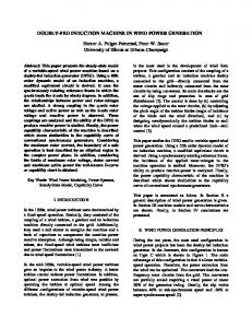
The doubly fed, twin stator, induction machine (DFTSIM) is being investigated as a variable speed drive [1,2]. One of the benefits of the DFTSIM is it exhibits synchronous behaviour at a pre determined, user settable, variable speed using a variable frequency converter of fractional rating. The rating of the converter is discussed in this paper. The DFTSIM being studied consists of two, nominally identical, wound rotor induction machines, shown schematically in Fig.1. The rotors of the machines are mechanically coupled and the rotor windings are connected so as to produce contra rotating magnetic fields in the separate machine sections. Because the two rotors are physically coupled, as depicted in Fig. 1, permanent connections may be made, rendering the brushes redundant except for providing a convenient means of measuring the rotor quantities. Under these conditions the DFTSIM is brushless. A number of studies have been conducted on the performance modelling of the brushless doubly fed machine (BDFM) [3-6], which is functionally equivalent to the DFTSIM.
I j L N p P ℘ ℜ R τ T V ω Z λ
RMS current (A) Imaginary operator Inductance (H) Mechanical speed (rpm) Differentiation with respect to time Number of pole pairs Power (W) Real part of complex quantity Resistance (Ω) Instantaneous torque (Nm) Steady state torque (Nm) RMS voltage (V) Angular velocity (rad/s) Impedance (Ω) Flux linkage (Wb)
B. Subscript and Superscript Variables c e g i l m M n out p r s *
Control machine Electrical Air gap Instantaneous Leakage Mechanical Mutual Natural Output Power machine Rotor Stator Complex conjugate
Bold lower case variable denotes instantaneous space phasor. Bold upper case variable denotes rms space phasor. Power winding refers to the stator winding of the power machine and control winding refers to the stator winding of the control machine.
In this paper, a positive control winding frequency denotes a balanced three phase set which produces a magnetic field that rotates in the same direction as that produced by the power winding voltages. A negative frequency denotes a voltage set that produces rotation Power machine
Control machine
Variable voltage, variable frequency supply
Utility supply : Fixed voltage and frequency
Fig.1 Arrangement of DFTSIM
[V ] = [V
in the opposite direction.
pc
The DFTSIM can operate in the synchronous mode, in which there is a single frequency of current in the rotor, and the rotor speed is a simple function of the stator supply frequencies and numbers of pole pairs, as follows:
Nm
(
)(
= 60 f p + f c / Pp + Pc
)
(1)
The natural or synchronous speed, Nn, occurs with dc applied to the control winding. This paper investigates the flow of power in the steady state using space phasors and makes comparison with the power flow in the BDFM [6].
Vc*
pc
T
pc
]
T
I*c
p
0
(Rcs − jω c Lcs ) jω r LcM
I r , and
jω p L pM − jω c LcM (Rr + jω r Lr )
Equation (4) contains voltages and currents at three separate frequencies. It may be transformed and written in terms of the power winding frequency only as ' [Vpc ] = [ Z 'pc ][ I pc ]
(5)
where
[V ] '
2. STEADY STATE EQUATIONS
[Z ] ' pc
= V p
Vc* s
T
0 ,
[I ] = [I pc
p
0 (R ps + jω p L ps ) Rcs = − jω p Lcs 0 s jω p LcM jω p L pM
I *c
]
T
I r , and
jω p L pM − jω p LcM Rr + jω r Lr s p
The slip terms are defined in Appendix A. Vp Ip i pR ps R ps jω p Llps
The general equation for the DFTSIM, in the rotor reference frame can be written as
[v] = [Z ][i]
] [I ] = [I
0 ,
(R ps + jω p L ps ) 0 jω r L pM
[Z ]=
pc
In the analysis, the following assumptions were made: (a) Balanced three phase windings are distributed to produce sinusoidal space variation of flux density; (b) Only the fundamental components of voltage and current are considered; (c) The magnetic circuits are linear, i.e. the effects of saturation and hysteresis are neglected; (d) Zero sequence quantities are not present; (e) The only losses are copper losses; (f) The rotors of the two machines are mechanically coupled with their ‘a’ phases aligned and the windings are connected in reverse sequence so as to produce contra rotating fields that are coincident on the magnetic axis of the ‘a’ phase.
p
jω p L pM
(2)
where
[v] = [v p
v *c
[i] = [i p
]
T
0 ,
R ps + ( p + jPpω m )L ps 0 pL pM
[Z ] =
i*c
0 Rcs + ( p − jPcω m )Lcs pLcM
]
jω p Llr
T
ir ,
(p + jP ω )L p
m
pM
( p − jPcω m )LcM (Rr + pLr )
Ir
Rr sp
Rr = R pr + Rcr , and Lr = L pr + Lcr . jω p LcM
The electromagnetic torque is given by
τe =
(
)
3 3 ℜ jPp L pM i *ps i pr + ℜ(− jPc LcM i cs i pr ) 2 2
(3) − jω p Llcs
where the first term represents the torque contributed by the power machine and the second the torque contributed by the control machine. Vc* s
In steady state, (2) becomes, using rms values
[Vpc ] = [ Z pc ][I pc ] where
(4)
Rcs s I*c
Fig.2 Steady state per-phase equivalent circuit
In steady state, the electromagnetic torque becomes, using rms values,
)
(
Te = 3 ℜ jPp L pM I*p I r + 3ℜ(− jPc LcM I c I r )
(6)
Equation (5) may be represented graphically by the equivalent circuit shown in Fig.2. 3. POWER FLOW In this section the per phase power will be discussed. To obtain the total power the per phase power is multiplied by three. Equation (5) contains electrical quantities that have been transformed to the utility supply frequency. It may be used for general steady state circuit calculations. To gain a clearer understanding of the power flow into the DFTSIM, (4) is used. It contains electrical quantities at the untransformed frequencies. The first row, relating to the power winding quantities, is at the utility frequency. The second is at the control winding frequency and the third is at the rotor electrical frequency. Multiplying the first row of (4) by Ir*, and taking the real part only gives
ℜ(V I
* p p
)− I
2 p
R ps − ℜ( jω p L pM I I
* r p
)= 0
(7)
The first term of (7) represents the power flowing into the power winding. The second term represents the power winding copper loss and the third the power machine air gap power. Multiplying the second row of (4) by Ic, and taking the real part only gives
ℜ(Vc*I c )− I c Rcs − ℜ(− jω c LcM I r I c ) = 0 2
(8)
The first term of (8) represents the power flowing into the control winding and it is noted that this is at the control frequency. The second term represents the control winding copper loss and the third is the control machine air gap power. Multiplying the third row of (4) by Ir*, and taking the real part only gives
0 = I r Rr + ℜ( jωr LpM I*r I p ) + ℜ(− jωr LcM I r I c ) 2
(9)
The electrical quantities in (9) are at the frequency of the rotor currents and voltages. Using the slip relationships in Appendix A, (9) may be rewritten as 0 = − I r Rr 2
[( − [ℜ( jP ω
)
] I I )]
+ ℜ jω p L pM I *p I r + ℜ(− jPcω m LcM I r I c ) p
m
)
L pM I I + ℜ(− jω c LcM * p r
r c
(10)
The first term in (10) is the rotor copper loss, the second is the power machine air gap power, the third the control machine air gap power and the final two
terms represent the mechanical output power. It is noted that in (7)-(10) power inputs are positive and the power outputs are negative. Equations (7)-(10) are similar to those for the BDFM [6], although [6] uses a slightly different dynamic model, defines positive sequence on the control winding opposite to that used in this paper and uses the symmetrical component transformation method in its development. The power delivered to the rotor is the sum of the air gap powers from the power and control windings and is
(
)
℘in = ℜ jω p L pM I*p I r + ℜ(− jω c LcM I r I c )
(11)
The total output power is the sum of the contributions from each part of the DFTSIM and is
(
)
℘out = ℜ jPpω m L pM I *p I r + ℜ(− jPcω m LcM I r I c ) (12)
Using the slip relationships in Appendix A, the output power may be represented as s ℘out = (1 − s p )℘pg + 1 + p ℘cg s
(13)
The first term in (13) is the same as the power output for a singly fed induction machine. In a standard induction machine the remainder of the air gap power, ℘pgsp, becomes the I2R loss. In the DFTSIM this is not the case. Only part of the ℘pgsp power is lost, the residue is transferred via the rotor to augment the power fed in from the control winding. This reduces the power processed by the converter meaning it can have a reduced rating beyond that dictated by the ratio of the number of poles on the control machine to the total number of poles. The quantity sp℘pg−Ir2Rpr can be a significant component of the power output of the control machine. 4. SIMULATION The machine parameters used in the simulations were those of a laboratory DFTSIM set consisting of two, nominally identical, wound rotor induction machines, ∆/Y connected, 6 pole, 1.5 kW, 15 Nm, 100 V, 50 Hz, 14.8 A. The parameters of the machines, calculated at 50 Hz, are: Rs=0.627 Ω, X1=1.20 Ω, Xm=18.0 Ω, Rr=1.29 Ω, X2=1.73 Ω, stator to rotor turns ratio=1.06, and J=0.31 kgm2. In all simulations, rated voltage and frequency were applied to the power winding. The simulations considered speeds corresponding to ±50 Hz on the control winding, corresponding, from (1), to a speed range of 0-1000 rpm. Simulations were carried out using the voltage controlled model described by (5), with control winding voltage as the control variable. The phase of the control winding voltage was such as to produce maximum torque at any speed.
For all speeds within this range power flows into the power winding and across the air gap. Power also flows, via the rotor, from the power machine to the control machine. At speeds above the natural speed
N n = 60 f p / (Pp + Pc )
(14)
It was expected the control winding air gap power and the control winding power would be positive [6]. Fig.3(a) shows the variation of control winding voltage and Fig.3(b) the air gap powers with load torque at 600 rpm. The control winding voltage is negative for torques below about 5 Nm. It can be seen that if the load torque is below a certain value, in this case about 25 Nm, the control winding air gap power is negative. Above this value power is needed from the control winding and correspondingly the air gap power is positive. The power inputs to each section of the machine are shown in Fig.3(c), from which it can be seen that for torques up to about 5 Nm a very small quantity of power is returned to the supply via the control winding, this being the torque the power machine alone can support. For torques above this value a relatively small quantity of power is fed into the control winding. From Fig.3(c) it can be seen that the bulk of the power is from the power winding and is unprocessed. Even when the torque is 25 Nm the VA being handled by the control winding is about 5% of that entering the power winding. Similar results were obtained at speeds below the natural speed. Fig.3(e) shows the control winding voltage characteristic whilst Figs.3(f) and (g) show the power and control machine powers. The control winding air gap power can be seen to be positive for torques up to about 10 Nm, while the control winding input power is positive up to nearly 26 Nm, this again being the torque that can be supported by the power machine alone. The difference in the positive and negative values for power at 600 and 400 rpm is caused by the reversal of the phase sequence of the control winding quantities at the natural speed. At speeds close to the natural speed the magnitude of the control winding voltage is small. The control winding voltage increases with torque as the speed difference between the natural speed and the operating speed increases. The voltage rating of the machine is exceeded at speeds below 140 rpm if the torque is maximal. Correspondingly the currents are also excessive at this speed and torque. The torque capability at 400 rpm is greater than at 600 rpm. This is true in general, the lower the speed the greater the torque capacity. For all values of torque considered the control machine air gap power is relatively small, compared with its power machine
counterpart. Although the sign and magnitude of the control winding powers varies with speeds above and below the natural speed the power winding power quantities can be seen to increase with load torque. For both speeds considered the control winding VA requirement is only a small fraction of the power machine VA contribution. The currents in each part of the machine are significant even at low torque. Figs.3(d) and (h) show the magnitudes of the currents for 600 rpm and 400 rpm respectively. In each case the control winding and rotor currents are within their rating but the power winding rating is exceeded at low values of torque at 600 rpm, mainly because of the magnetizing current, which is in excess of 5 A, about 30% of the rated winding current. The VA rating of the control winding converter will increase at low speed and high torque, the limiting factor being the winding current and not the voltage. For example, at a speed of 100 rpm and with load torque up to 35Nm the control winding VA is less than 1kVA whilst the power winding handles more than five times this amount. 5 CONCLUSIONS Equations describing the flow and distribution of power in the DFTSIM have been developed using a space phasor model. Simulation studies, based on a laboratory set comprising two nominally identical wound rotor induction motors have been presented. It has been shown that, at the speeds considered, the power and VA rating of the control machine converter is small compared to entering the power winding. It has also been shown that power can be regenerated at speeds above and below the natural speed of the DFTSIM. Further studies are planned to evaluate the performance limits and efficiency of the DFTSIM.
REFERENCES [1] N. Chilakapati, V.S. Ramsden, V. Ramaswamy, and J.G. Zhu, “Investigation of Doubly Fed Twin Stator Induction Motor as a Variable Speed Drive”, Proc. International Conference on Power Electronics Drives and Energy Systems for Industrial Growth (PEDES), 1998, pp.160-165 [2] N. Chilakapati, V.S. Ramsden, V. Ramaswamy, and J.G. Zhu, “Comparison of Closed-loop Speed Control Schemes for a Doubly Fed Twin Stator Induction Motor Drive”, Proc. International Power Electronics and Motion Control Conference (IPEMC) 2000, pp.786-791
Voltage (V) 15
15
10
10
5
5
Voltage (V)
0
0 0
5
10
15
20
0
25
5
10
15
20
25
30
35
40
-5
-5
-10
-10
-15
-15 Torque (Nm)
Torque (Nm)
(a) Control winding voltage vs. torque at 600 rpm
(e) Control winding voltage vs. torque at 400 rpm
Power (W) 3000
Power (W) 3000
2500
2500
Power winding Power winding
2000
2000
1500
1500
1000
1000
500
500 Control winding 0
5
10
15
Control winding
0
0 20
25
0
5
10
15
20
25
30
35
40
-500
-500
Torque (Nm)
Torque (Nm)
(f) Air gap powers vs. torque at 400 rpm
(b) Air gap powers vs. torque at 600 rpm
Power (W) 3500
Power (W) 3500
3000
3000
Power winding
2500
2500
Power winding
2000 2000
1500
1500
1000
1000
500
500
0
Control winding
-500
0 0
5
10
15
20
25
-500
Control winding 0
5
10
15
20
25
30
35
40
-1000 Torque (Nm)
Torque (Nm)
(g) Input powers vs. torque at 400 rpm
(c) Input powers vs. torque at 600 rpm
Current (A) 18
Current (A) 18
16
16 Power winding 14
Rotor
Power winding
14 12
12 Control winding
10
Rotor
10
8
8
6
6
4
4
2
2
Control winding
0
0 0
5
10
15
20
25
0
5
10
15
20
25
30
35
Torque (Nm)
Torque (Nm)
(d) Winding currents vs. torque at 600 rpm
(h) Winding currents vs. torque at 400 rpm
Fig.3 Voltage, power and current vs. torque
40
[3] R. Li, R. Spée, A. Wallace, and G. C. Alexander, “Synchronous Drive Performance of Brushless Doubly-Fed Motors”, IEEE Trans. on Industry Applications, Vol.30, No.4, 1994, pp.963-970 [4] S. Williamson, A. C. Ferreira and A. K. Wallace, “Generalised theory of the brushless doubly-fed machine. Part 1: Analysis”, IEE Proc. Electrical Power Applications, 1997 144 (2), pp.111-121 [5] S. Williamson, and A. C. Ferreira, “Generalised theory of the brushless doubly-fed machine. Part 2: Model verification and performance”, IEE Proc. Electrical Power Applications, 1997 144 (2), pp.123-129
By this definition, the slip for the power machine can be expressed consequently as sp =
ω p − Ppω m ωp
(A2)
and the slip for the control machine
sc =
ω c − Pcω m ωc
(A3)
The slip for the DFTSIM is defined to be s=−
sp sc
=
(ω
p
− Ppω m )
ωp
ωc
(Pcω m − ωc )
=
ωc ωp
(A4)
Because [6] B.V. Gorti, G.C. Alexander, and R. Spée, “Power Balance Considerations for Brushless Doubly-Fed Machines”, IEEE Trans. on Energy Conversion, Vol.11, No.4, Dec. 1996, pp.687-692 APPENDIX A. DEFINITIONS OF SLIP
Synchronou s speed − Rotor speed Synchronou s speed
(A5)
and
ω r = −ω rc = −(ω c − Pcω m )
(A6)
we have
In a single stator induction machine, the slip, s, is defined as s=
ω r = ω rp = ω p − Ppω m
(A1)
Ppω m = ω p (1 − s p ) and s Pcω m = ω c 1 + p s
(A8) (A9)