Power Maximization and Control of Variable-Speed Wind Turbine

Journal of Power and Energy Engineering, 2018, 6, 51-69 http://www.scirp.org/journal/jpee ISSN Online: 2327-5901 ISSN Print: 2327-588X

Power Maximization and Control of Variable-Speed Wind Turbine System Using Extremum Seeking Safanah M. Rafaat, Rajaa Hussein Control and Systems Engineering Department, University of Technology, Baghdad, Iraq

How to cite this paper: Rafaat, S.M. and Hussein, R. (2018) Power Maximization and Control of Variable-Speed Wind Turbine System Using Extremum Seeking. Journal of Power and Energy Engineering, 6, 51-69. https://doi.org/10.4236/jpee.2018.61005 Received: December 12, 2017 Accepted: January 27, 2018 Published: January 30, 2018 Copyright © 2018 by authors and Scientific Research Publishing Inc. This work is licensed under the Creative Commons Attribution International License (CC BY 4.0). http://creativecommons.org/licenses/by/4.0/ Open Access

Abstract Maximizing the power capture is an important issue to the turbines that are installed in low wind speed area. In this paper, we focused on the modeling and control of variable speed wind turbine that is composed of two-mass drive train, a Squirrel Cage Induction Generator (SCIG), and voltage source converter control by Space Vector Pulse Width Modulation (SPVWM). To achieve Maximum Power Point Tracking (MPPT), the reference speed to the generator is searched via Extremum Seeking Control (ESC). ESC was designed for wind turbine region II operation based on dither-modulation scheme. ESC is a model-free method that has the ability to increase the captured power in real time under turbulent wind without any requirement for wind measurements. The controller is designed in two loops. In the outer loop, ESC is used to set a desired reference speed to PI controller to regulate the speed of the generator and extract the maximum electrical power. The inner control loop is based on Indirect Field Orientation Control (IFOC) to decouple the currents. Finally, Particle Swarm Optimization (PSO) is used to obtain the optimal PI parameters. Simulation and control of the system have been accomplished using MATLAB/Simulink 2014.

Keywords Wind Turbine, Indirect Field Orientation Control (IFOC), Maximum Power Point Tracking (MPPT), Extremum Seeking Control (ESC), Particle Swarm Optimization (PSO), PI Controller

1. Introduction Wind energy is a fast-growing interdisciplinary field that encompasses multiple branches of engineering and science. Wind energy has gained tremendous attenDOI: 10.4236/jpee.2018.61005

Jan. 30, 2018

51

Journal of Power and Energy Engineering

S. M. Rafaat, R. Hussein

tion over the past two decades as one of the most promising renewable energies for the future, environmentally friendly solutions, pollution-free and inexhaustible sources [1]. According to speed control, WTs are classified into two types: fixed and variable speed WT. Fixed speed turbines are using SCIG directly connected to grid without using power electronic converters. The speed of the generator is constant regardless of the wind speed. Variable-speed turbines are currently the most used turbines that use different types of generators connected to grid through the power converters. Variable-speed turbines allow the rotational speed to be continuously adapted and controlled in such a manner that the turbine operates constantly at its highest level of aerodynamic efficiency then the maximum energy can be extracted relying upon the wind speed variations. Maximizing power capture for variable speed Wind Turbine (WT) by means of control theory has been a popular topic for the researchers. According to WT operation regions that will be explained in the next section, the researchers applied different control methodologies by using generator speed control to harvest maximum energy in region II, using blade pitch control to reduce mechanical loads and maintenance cost in region III, or a combination of both. Model-based strategies have been studies for region II control [2] [3] [4]. The model-based control approaches can achieve good performance for some ranges of operating conditions but these methods have some limitations and difficulties as the mathematical model of the system is directly incorporated into the controller. Thus, the controller incorporates knowledge of how the system dynamics change with the operating conditions. The Wind Energy Conversion Systems (WECS) are very complex and it’s difficult to obtain the dynamics equations otherwise, model-based methods required experimental data and/or lookup tables under specific wind condition and accurate wind speed measurement. To overcome some difficulties with model-based control methods and reduce the dependency on the mathematical model, other researchers proposed different model-free control methods for Region II operation. Johnson et al. [5] proposed Model Reference Adaptive Control (MRAC), he maximized output power by selecting a suitable control law that related the speed directly with torque then MRAC adapted the torque gain to increase power. Barakati et al. [6] proposed classical MPPT methods, like model-free Perturbation and Observation (P & O) method. The logic of this method is to perturb control input with a certain step size and observe the change in power output. In this paper, Extremum Seeking Control (ESC) scheme [7] [8] for WT region II operation was proposed to maximize the output power capture without consideration of the load impacts. ESC is a nonmodel-based self-optimizing control strategy that aims to search for unknown input in real-time varying systems by finding the extreme point. The plant excited with some sinusoidal probing signals (dither signal). ESC is applicable in situations where there is nonlinearity in the control problem, and the nonlinearity has local minimum or a maximum. DOI: 10.4236/jpee.2018.61005

52

Journal of Power and Energy Engineering

S. M. Rafaat, R. Hussein

Creaby et al. [9] used ESC method to maximize the rotor mechanical power. They used sinusoidal signal as a dither perturbation signal and second order filters to seek the maximum point. Ghaffari and Krstic et al. [10] used the same method with first order filters. Xiao et al. [11] presented the experimental works to the same model that used by Creaby (CART3 facility). In this work, both schemes have been considered. Moreover, maximization of the electrical power has been worked on in order to produce more accurate results than maximization of the mechanical power. The approach in this paper focuses on the control of variable speed WT composed of two-mass drive train, SCIG, and voltage source converter control by SPVWM. The controller is designed in two loops, in the outer loop ESC has been used to set a desired reference for PI control of the generator speed and extract the maximum electrical power within high wind speed variation. The inner control loop is based on IFOC for the currents decoupling. The following Sections are organized as a follow. In Section 2, the design of wind energy conversion system has presented with concentration on the dynamic equations of SCIG in dq reference frame and two-mass drive train. In Section 3, the controller design was discussed. In Sections 4 and 5, Simulation results and conclusions are presented respectively.

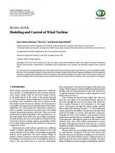
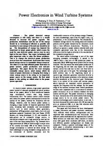
2. Wind Energy Conversion System Model 2.1. Aerodynamics Model WT is composed of different parts to achieve kinetic-to-electric energy conversion. The wind kinetic energy is converted to mechanical energy by the blades. The mechanical energy is transmitted through the drive train to the generator, which converts mechanical energy into electric energy. This conversion is supported by power converters that deliver the power from the generator to the grid, as shown in Figure 1 [12]. The physical definition for kinetic energy is

1 KE = mV 2 2

(1)

But the power definition P is the kinetic energy per unit time:

= P

1 1 dm 2  2 = mV V 2 2 dt

(2)

where, V is the speed and m is the air mass that passes the disc of wind turbine rotor in a unit length of time, e.g., m = ρ AV∞ Thus, the available power in the wind stream is

Pavail =

1 ρ AV∞3 0.5πρ Rt2V∞3 = 2

(3)

where Pavail is the wind power, ρ is the air mass density, πRt2 = A is the swept area of turbine rotor, and V∞ is the wind speed. The mechanical power that can be extracted from the wind power is DOI: 10.4236/jpee.2018.61005

53

Journal of Power and Energy Engineering

S. M. Rafaat, R. Hussein

Figure 1. Wind turbine components [1].

Pmech = Pavail C p ( λ , β )

(4)

where, C p ( λ , β ) is, the power coefficient, the ratio of the mechanical power

to available power, β is the pitch angle of the blade, and λ is the Tip-SpeedRatio (TSR) can be obtained by

λ=

Ω wtr Rt V∞

(5)

where, Ω wtr is the low-speed shaft and Rt is turbine rotor radius. Wind turbine operation regions are typically divided into four primary regions, as seen in Figure 2. Region 1 spans operation from startup to the cut-in wind speed. In Region 2 the turbine is said to be in sub-rated region when wind speeds are between cut-in and rated speed. The primary goal is to capture as much power as possible. In Region 3 wind speeds are high enough to drive the generator at its rated power output; in this case, the goal is to regulate speed and power safely at rated levels. Region 4 occurs when the turbine shuts down to prevent damage due to high wind speeds [13].

The quantity C p ( λ , β ) is a nonlinear function, difficult to measure and

predict, has different values between each turbine and another depending on turbine parameters and design. The theoretical upper limit for C p is Betz Limit equals to 0.59. The C p is obtained based on the exponential function in [14]. DOI: 10.4236/jpee.2018.61005

54

Journal of Power and Energy Engineering

S. M. Rafaat, R. Hussein

Figure 2. Wind turbine operation regions.  −21  λi 

 116   C= 0.5176  − 0.4 β − 5  ∗ e p (λ, β )  λi 

+ 0.0068λ

(6)

1 1 0.035 where, = − 3 . λ i λ + 0.08β β + 1

The power coefficient C p ( λ , β ) is a function of blade bitch angle and tip speed ratio. The maximum value of C p equals to 0.479 at β = 0 and λ = 8 , so for region II operation, the pitch angle is settled to zero and the C p is now a function of TSR only C p ( λ ) . Then, the obtained power coefficient is shown in Figure 3(a) and Figure 3(b).

2.2. Dynamic Equations for Two-Mass Model Drive Train The model has two masses corresponding to WT rotor and generator, respectively. The dynamic equations of motion for the drive-train are written with respective to the generator mass as given below. Table 1 illustrates all parameters definitions [15].

′ ′ = Twtr J wtr

dΩ wtr ′ ( Ω′wtr − Ω gen ) + K shaft ′ (θ wtr ′ − θ gen ) + Dshaft dt

= −Tgen J gen

dΩ gen dt

′ ( Ω gen − Ω′wtr ) + K shaft ′ (θ gen − θ wtr ′ ) + Dshaft ′ dθ wtr = Ω′wtr dt

dθ gen dt DOI: 10.4236/jpee.2018.61005

55

= Ω gen

(7) (8) (9) (10)

Journal of Power and Energy Engineering

S. M. Rafaat, R. Hussein

0.5 0.4 0.5

←2 ←3 ←4

Power Coefficient

0.3 0.2

-0.2

←1 ←6 ←7 ←8 ←9 ←10 ←11

-0.3

←13

-0.4

←14 ←15

0.1 0 -0.1

-0.5

0

←0

0

5

10

15

15 -0.5 15

Lambda

(a)

10 10

5

5

0

0

(b)

Figure 3. (a) C p ( λ , β ) in 2D, (b) C p ( λ , β ) as a surface. Table 1. Parameters and variables of the drive train are referred to generator mass. Parameters

Description

Unit

Referred to the mass of the generator

k gear

Gearbox ratio

J gen

Generator inertia

kg·m2

J wtr

Wind turbine rotor inertia

kg·m2

′ = J wtr

J wtr k gear

K shaft

Shaft stiffness

N·m/rad

′ = K shaft

K shaft

Dshaft

Shaft damping coefficient

N·m·s/rad

′ = Dshaft

Dshaft

Tgen

Generator torque

N·m

Twtr

Wind turbine rotor torque

N·m

′ = Twtr

Twtr k gear

Ω gen

Speed of the high speed shaft

rad/s

Ω wtr

Speed of the low speed shaft

rad/s

θ gen

High speed shaft angular position

rad

θ wtr

Low speed shaft angular position

rad

Tshaft

Internal shaft torque

N.m

2 k gear

2 k gear

Ω′wtr= k gear ⋅ Ω wtr ′ = k gear ⋅ θ wtr θ wtr

2.3. Squirrel Cage Induction Generator (SCIG) Model The dynamic equations of induction machine in reference frame can be written using either fluxes, currents or both as state-variables. The four loop equations described from the equivalent circuits where the variables ids , iqs , idr and iqr represent the state variables and Vds , Vqs , Vdr and Vqr represent the input vector of the state-space model in the dq reference frame. So, the state and input vectors are respectively: DOI: 10.4236/jpee.2018.61005

56

Journal of Power and Energy Engineering

S. M. Rafaat, R. Hussein

ids = x = x1 ( t ) x2 ( t ) x3 ( t ) x4 ( t )  T

u = Vds

Vqs

Vqr 

Vdr

iqs

iqr 

idr

T

T

(11) (12)

For SCIG, the d and q components of the rotor voltage set to zero, i.e.

(V= Rd

0 ) since the rotor of squirrel cage machine has slot-embedded bars V= Rq

that are shorted by end rings. The nonlinear fourth-order state model of SCIG can be presented as in the equations below [3] [16].

X = A ( Ω gen ) ⋅ X + B ⋅ u Y= ≡ Tgen = Tgen

3Pp Lm 2

3Pp Lm 2

(i

(13)

( x2 x3 − x1 x4 )

(14)

i − ids iqr )

(15)

qs dr

where,

 Pp Ω gen L2m Rs ω − +  s σ Ls σ Ls Lr    2 R  −  ω + Pp Ω gen Lm  − s s    σ Ls Lr  σ Ls A ( Ω gen ) =    Pp Ω h Lm Lm Rs −  σ Ls Lr σ Lr   Pp Ω gen Lm Rs Lm   σ Lr σ Ls Lr

Lm Rr σ Ls Lr −

Pp Ω gen Lm

σ Ls −

Rr σ Lr

−ωs +

Pp Ω gen

σ

Pp Ω gen Lm   σ Ls   Lm Rr  σ Ls Rr   Pp Ω gen  ωs −  σ   R  − r σ Lr  (16)

 1 σ L s B=   0 

0

− Lm

σ Ls Lr

1 σ Ls

0

   − Lm   σ Ls Rr 

T

0

(17)

while, the Equation (15) can be rewritten with rotor flux variables instead of rotor current as in Equation (18) to be prepared for IFOC. Tgen =

3Pp Lm 2 Lr

(i ψ qs

dr

− idsψ qr )

(18)

2.4. Voltage Source Converters and Space Vector PWM Electrical generators are usually controlled by power electronics converters. Power converters are controlled using a switching strategy. Space vector modulation (SVM) is one of the preferred real-time modulation techniques and it is widely used for digital control of voltage source converters. SVM allows reducing commutation losses and the harmonic distortion of output voltage waveform, giving higher amplitude modulation indexes. The SVM control is designed space vector combinations to get a reference voltage Vref . The summation of the voltage multiplied by the time interval of chosen space vectors equal the product DOI: 10.4236/jpee.2018.61005

57

Journal of Power and Energy Engineering

S. M. Rafaat, R. Hussein

of the reference voltage Vref and sampling period Tz by knowing in which sector the reference voltage vector is located, we select the two adjacent basic voltage space vectors and one zero-vector. For example, when Vref falls into Sector I, it can be synthesized by V1 , V2 and V0 that gives the equation below. The detail explanation is found in [17] and its references, where our implementation is done based on them. Vref Tz V1T1 + V2T2 + V0T0 =    Tz = T1 + T2 + T0

(19)

3. Wind Energy Conversion System Control 3.1. Field Orientation Control (FOC) FOC can be classified in two design approaches 1) Direct FOC and 2) Indirect FOC, according to the implementation method that is used to estimate the rotor flux ψ r and the synchronous position θ s . The rotor flux orientation is one of the most popular schemes used in AC drives control and WECS control due to its simple and easy implementation. The necessity of using FOC is the decoupled control of the rotor flux and electromagnetic torque of the machine to achieve high dynamic performance. The synchronous frequency equals to the summation of machine rotor frequency ωr and slip frequency ωsl then by the integration of them, the position θ s can be obtained.

θ s =∫ ωs =∫ (ωr + ωsl ) = θ r + θ sl

(20)

For rotor flux orientation, the mathematical model of the SCIG in d-q frame is given in Equations (11)-(18). The decoupling control can be achieved by aligning the stator flux component of the current ids on the d-axis, and the torque component of the current iqs should align the q-axis, that leads to ψ dr = 0 ,

ψ dr = ψ r [3] [12] [16] [18]. Then,

(i ψ )

(21)

Lr dψ r +ψ r = Lmids Rr dt

(22)

Tgen =

3Pp Lm 2 Lr

qs

dr

3.2. Extremum Seeking Control (ESC) A new method for driving the operating point to the energy maximum, based on Extremum Seeking (ES) was introduced to overcome challenges with the conventional MPPT algorithm and remove the dependence of the plant modeling. ESC is a class of self-optimizing control strategy which can search for unknown time varying input for optimizing a performance index of nonlinear plant. In this Work, the electrical power was used as the performance index

and our objective is to maximize this function f ( u ) by a proper selection of dither signal frequency ω , Low Pass Filter (LPF) frequency ωl and High Pass Filter (HPF) frequency ωh , and integrator gain k to set the control uˆ DOI: 10.4236/jpee.2018.61005

58

Journal of Power and Energy Engineering

S. M. Rafaat, R. Hussein

in the real time. ESC is interpreted as single-input setting with dither signal (usually sinusoidal signal S ( t ) ) added to the estimated uˆ . The schematic diagram of whole variable speed WT including control system, mechanical and electrical components, and MPPT method using ESC is shown in Figure 4 [8] [11]. The input and the output to plant become:

u= uˆ + cos (ωt )

(23)

y f ( uˆ + cos (ωt ) ) =

(24)

where, ω is the dither frequency equals to 20.6 rad/s. Then Taylor series expansion for Equation (24) becomes:

y= f ( uˆ + cos (ωt ) ) = f ( uˆ ) + cos (ωt )

∂f + H .O.T ∂u

(25)

HPF filters out the DC term while passes the AC term then by multiplying with the demodulation signal M ( t ) = cos (ωt ) , that yields:

∂f   ∂f cos (ωt ) ×  cos (ωt ) + H .O.T  =+ H .O.T ∂u   ∂u

(26)

LPF retains DC term to estimate the gradient of the objective function with respect to the control input u while filters out AC term from Equation (26). The loop is closed with an integrator to drive the gradient to zero in steady state. Several signals were examined as dither signals for ESC. The cosine signal was applied as a harmonic signal and wind speed signal was applied as non-harmonic signal. In addition, the HPF and LPF have been implemented in both as 1st and 2nd order transfer functions. The 1st and 2nd order transfer function for HPF is given below with cutoff frequency ωh = 3 rad/s: = G1st_HPF

s s2 = , G2nd_HPF s + ωh s 2 + 2 × 0.58 × ωh s + ωh2

(27)

Figure 4. Schematic diagram of variable speed WT control system. DOI: 10.4236/jpee.2018.61005

59

Journal of Power and Energy Engineering

S. M. Rafaat, R. Hussein

The 1st and 2nd order transfer function for LPF is given below with cutoff frequency ωl = 8 rad/s:

ω

G1st_LPF =

ω2

(28)

l l , G2nd_LPF = s + ωl s 2 + 2 × 0.6 × ωl s + ωl2

By feedbacking the electrical power to ES, the optimal speed value is obtain to achieve the maximum energy captured. Different types of dither signals have been examined to get the best reference speed to the system since the selection of the dither signal is an important issue in the application of ESC [19] [20]. Figure 5 shows the effect of choosing different type of dither signals to generate the reference speed. The response in blue color (using 1st order filters and cosine signal as dither signal for ES) suffers from ripples and rises above the optimal speed 157.5 rad/s in the periods (16 - 20 s), while the responses in green (using 2nd order filters and cosine signal as a dither signal for ES) and pink (using 2nd order filters and wind signal as a dither signal for ES) have high overshoots at 0.5 s. Moreover the green response is decreasing to 156.5 rad/s at 16 s. The response in red color (using 1st order filters and wind signal as a dither signal for ES) was found to be the best to choose as a reference speed.

3.3. Optimized PI Control Using Particle Swarm Optimization The PI controller is the more commonly used control strategy in electrical machines for speed control. There are many different algorithms to find suitable parameters of the controller. To achieve the closed loop speed control, we firstly select one of the generated speed references from the above sub-section to be the speed command for PI controller. The PI parameters are found using trial and error method to control the speed of generator then Particle Swarm Optimization (PSO) has been presented to determine the optimal PI parameters and ensure the maximum power captured. PSO is an off-line optimization algorithm based on population. PSO algorithm gives high quality solutions and stable 180 160

Speed-ref (rad/sec)

140

170

159

120

165

100 80

160

60

155

40

150 0

20 0

spd-ref ESC 1st-cos 158 spd-ref ESC 2nd-cos spd-ref ESC 1st-wind spd-ref ESC 2nd-wind 157

0

1

2

2

4

156 16

3

6

8

10

12

14

18 16

20 18

20

Time (sec)

Figure 5. The generator reference speed using different types of dither signals. DOI: 10.4236/jpee.2018.61005

60

Journal of Power and Energy Engineering

S. M. Rafaat, R. Hussein

convergence characteristics within shorter calculation time. In PSO, particles fly around in a multidimensional search space then during its flight each particle adjusts its position according to its own experience (P-best), and according to the experience of a neighboring particle (G-best), made the best position encountered by itself and its neighbor [21]. The velocity of each agent can be modified by the following equation:

(

)

(

= V k +1 inertia ⋅ V k + c1 ⋅ rand ⋅ Pbest − x k + c2 ⋅ rand ⋅ Gbest − x k

)

(29)

The current position can be modified by the following equation: 1 x k += x k + V k +1

(30)

The performance index (ITSE) is chosen as cost function for PSO and given by.

ITSE =

∞

∫0 t ⋅ e ( t )

2

(31)

dt

As mentioned before, the closed loop control for regulating the speed of the generator had accomplished using PI controller. The gain values for Kp and Ki were tuned manually then improved using PSO. The presented data in Figure 6 and Table 2 had been obtained at the following values: iteration = 20, swarm size = 30, inertia = 0.9, and c= c= 2. 1 2

4. Simulation Results The modeling of variable speed wind turbine for mechanical and electrical components has been built based on Equations (1)-(17), the currents of the Table 2. PI control parameters for generator speed control. The applied method

Kp

Ki

PI gains tuned using trial and error

2100

1000

PI gains tuned using PSO algorithm

2199.0295

1093.6790

180

Generator speed (rad/sec)

160 140 120

159

160

158

150

157

100 140

156

130 0

155 16

80 60 40 20 0 0

1 161 160

2

3

4

5

18

17

19

20

spd-ref ESC 1st-wind spd-gen trial and error spd-gen tuned by pso

159 2

2.2

2

4

2.4

2.6 6

8

10 Time (sec)

12

14

16

18

20

Figure 6. Tuning of PI controller to control the speed of the generator. DOI: 10.4236/jpee.2018.61005

61

Journal of Power and Energy Engineering

S. M. Rafaat, R. Hussein

squirrel cage induction generator is decoupled using IFOC based on Equations (18)-(22) and ESC was presented as explained before. MATLAB/Simulink block diagram is shown in Figure 7, also the data of 2 MW wind turbine are found in Appendix A. The input signal to the whole model is the wind speed which has been modeled and developed based on the Kaimal spectra in [15] [22]. Figure 8 shows the obtained signal. The Simulation has been solved using fixed-step ode4 solver with sampling −5 time τ s = 1e . The initial values for the speed of generator (high-speed shaft)

(

)

and the speed of turbine rotor (low-speed shaft) are 156.5, 1.874 rad/s respectively.

Figure 7. Simulink block diagram of variable speed wind turbine based on SCIG. 13

Wind speed (m/sec)

12 11 10 9 8 7 0

2

4

6

8

10 Time (sec)

12

14

16

18

20

Figure 8. The obtained wind speed signal based on kaimal spectra. DOI: 10.4236/jpee.2018.61005

62

Journal of Power and Energy Engineering

S. M. Rafaat, R. Hussein

The other parameters values are initially set to zero. Figure 9 and Figure 10 show that the mechanical power had been maximized as result of the approaching of power coefficient from its maximum value

(C

p

= 0.479 ) . ESC in the out-

er loop is based on the generator speed regulation via the electrical power feedback. The ESC searches for the optimal generator’s speed to maximize power without accurate knowledge of power map. In the inner loop, PI controller regulates the generator speed in closed loop to attain the optimal speed that is suggested by ESC. As in Figure 6, the speed of the generator was approximately around the optimal speed 157.5 rad/s, meanwhile the speed of turbine rotor in Figure 11 is around 2.1 rad/s since the gearbox ratio equals to 75. Figure 12 shows that the electrical power attains its maximum power capture in some periods of time (2 MW in 6 - 8 s, 14 - 19 s), meanwhile the electromagnetic torque in Figure 13 approaches to its rated value (14,700 Nm in same periods) according to the decreasing or increasing in wind speed measurements. Finally, Figure 14 shows the three phase stator currents of SCIG. 6

x 10 2

Mechanical power (W)

1.8 1.6 1.4 1.2 1 0.8 0.6 0.4 0

2

4

6

8

10 Time (sec)

12

14

16

18

20

12

14

16

18

20

Figure 9. Wind turbine mechanical power (Captured power). 0.5

Power coefficient (Cp)

0.45 0.4 0.35 0.3 0.25 0.2 0.15 0.1 0

2

4

6

8

10 Time (sec)

Figure 10. The power coefficient Cp. DOI: 10.4236/jpee.2018.61005

63

Journal of Power and Energy Engineering

S. M. Rafaat, R. Hussein

2.25

WT rotor speed (rad/sec)

2.2 2.15 2.1 2.05 2 1.95 1.9 1.85 0

8

6

4

2

12

10 Time (sec)

14

16

18

20

16

18

20

Figure 11. Wind turbine rotor speed (rad/s). 4

1.5

x 10

Generator Torque (N.m)

-5000 1

-5500 0.5 -6000 11

0

11.5

12

12.5

-0.5 -1 -1.5 0

2

4

6

8

10 Time (sec)

12

14

Figure 12. Electromagnetic torque (N·m). 6

4

x 10

5

x 10

Electrical power (W)

3

-4 -6 -8 -10 -12 10

2 1 0

10.2

10.4

10.6

14

16

10.8

11

-1 -2 -3 0

2

4

6

8

10 Time (sec)

12

18

20

Figure 13. Electrical power (Watt). DOI: 10.4236/jpee.2018.61005

64

Journal of Power and Energy Engineering

S. M. Rafaat, R. Hussein

Stator currents (Is-abc) Ampere

4000 2000 0 -2000 -4000 1000

1000

0

0 -1000

-6000

-8000 -1000 -10000 0

11 2

4

11.05 6

11

11.1 8

10 12 Time (sec)

11.5 14

12 16

18

20

Figure 14. The stator currents of the generator in three phase.

5. Conclusion In this paper, the development of MPPT with ESC to harvest maximum energy captured in the sub-rated speed region has been presented. The simulation results show the strength of ESC to get the position of the operating point neglecting the model dynamics equations as compared with the conventional MPPT methods that highly depend on the dynamic equations and speed measurements. For its being a self-optimizing model-free method, ESC has provided good convergence rate despite the time-varying in wind speed. The output electrical power was used as a performance index to the ESC scheme which shows more interest in energy capture than using the mechanical power. We examined different kinds of dither signals for ESC to achieve slow perturbation to the system and the non-harmonic wind signal with first order transfer function was the better one. The rotor flux orientation control was implemented in inner control loop to achieve the required decoupling between currents and electromagnetic torque. The PI gains values in speed control loop is tuned firstly by trial and error then improved with PSO, where the obtained parameters gains attain the optimal energy captured.

References

DOI: 10.4236/jpee.2018.61005

[1]

Pao, L.Y. and Johnson, K. (2011) Control of Wind Turbines: Approaches, Challenges, and Recent Developments. IEEE Control Systems Magazine, 31, 44-62. https://doi.org/10.1109/MCS.2010.939962

[2]

Abdullah, M.A., Yatim, A.H.M., Tan, C.W. and Saidur, R. (2012) A Review of Maximum Power Point Tracking Algorithms for Wind Energy Systems. Renewable and Sustainable Energy Reviews, 16, 3220-3227. https://doi.org/10.1016/j.rser.2012.02.016

[3]

Munteanu, I. and Bratcu, A.I. (2008) Optimal Control of Wind Energy Systems: Towards a Global Approach. Springer, Berlin.

[4]

Soliman, M., Malik, O.P. and Westwick, D.T. (2011) Multiple Model Predictive 65

Journal of Power and Energy Engineering

S. M. Rafaat, R. Hussein Control for Wind Turbines with Doubly Fed Induction Generators. IEEE Transaction on Sustainable Energy, 2, 215-225. https://doi.org/10.1109/TSTE.2011.2153217 [5]

Johnson, K.E., Fingersh, L.J., Balas, M.J. and Pao, L.Y. (2004) Methods for Increasing Region 2 Power Capture on a Variable-Speed Wind Turbine. Journal of Solar Energy Engineering. 126, 1092-1100. https://doi.org/10.1115/1.1792653

[6]

Barakati, S.M., Kazerani, M. and Aplevich, J.D. (2009) Maximum Power Tracking Control for a Wind Turbine System Including a Matrix Converter. IEEE Transactions on Energy Conversion, 24, 705-713. https://doi.org/10.1109/TEC.2008.2005316

[7]

Krstić, M. and Wang, H.H. (2000) Design and Stability Analysis of Extremum Seeking Feedback for General Nonlinear Systems. Automatica, 36, 595-601. https://doi.org/10.1016/S0005-1098(99)00183-1

[8]

Ariyur, K.B. and Krstić, M. (2003) Real-Time Optimization by Extremum-Seeking Control. John Wiley & Sons, Hoboken. https://doi.org/10.1002/0471669784

[9]

Creaby, J., Li, Y. and Seem, J.E. (2009) Maximizing Wind Turbine Energy Capture Using Multi-Variable Extremum Seeking Control. Wind Engineering, 33, 361-387. https://doi.org/10.1260/030952409789685753

[10] Ghaffari, A., Krstić, M. and Seshagiri, S. (2014) Power Optimization and Control in Wind Energy Conversion Systems Using Extremum Seeking. IEEE Transactions on Control Systems Technology, 22, 1684-1695. https://doi.org/10.1109/TCST.2014.2303112 [11] Xiao, Y., Li, Y.Y. and Rotea, M. (2016) Experimental Evaluation of Extremum Seeking Based Region-2 Controller for CART3 Wind Turbine. 34th Wind Energy Symposium, AIAA, Reston. https://doi.org/10.2514/6.2016-1737 [12] Wu, B., Lang, Y., Zargari, N. and Kouro, S. (2011) Power Conversion and Control of Wind Energy Systems. Wiley, Hoboken. https://doi.org/10.1002/9781118029008 [13] Aho, J., Buckspan, A., Laks, J., Fleming, P., Jeong, Y., Dunne, F., Churchfield, M., Pao, L.Y. and Johnson, K. (2012) A Tutorial of Wind Turbine Control for Supporting Grid Frequency through Active Power Control. American Control Conference (ACC), 3120-3131. [14] Reyes, V., Rodríguez, J.J., Carranza, O. and Ortega, R. (2015) Review of Mathematical Models of Both the Power Coefficient and the Torque Coefficient in Wind Turbines. IEEE 24th International Symposium on Industrial Electronics (ISIE), June 3-5 2015, Buzios, 1458-1463. https://doi.org/10.1109/ISIE.2015.7281688 [15] Iov, F., Hansen, A.D., Sorensen, P. and Blaabjerg, F. (2004) Wind Turbine Blockset in MATLAB/Simulink. Aalborg University, Denmark. [16] Bose, B.K. (2001) Modern Power Electronics and AC Drives. Prentice-Hall, Englewood Cliffs. [17] Cheng, J. and Wang, W. (2013) Simulation Study of Space Vector Pulse Width Modulation in Wind Power Generation System. 2013 International Conference on Materials for Renewable Energy and Environment (ICMREE), August 19-21 2014, Chengdu, 415-418. https://doi.org/10.1109/ICMREE.2013.6893696 [18] Shaija, P.J. and Elizabeth Daniel, A. (2016) An Intelligent Speed Controller Design for Indirect Vector Controlled Induction Motor Drive System. 25, 801-807. https://doi.org/10.1016/j.protcy.2016.08.177 [19] Tan, Y., Nešić, D. and Marlees, I. (2008) On the Choice of Dither in Extremum Seeking Systems: A Case Study. Automatica, 44, 1446-1450. https://doi.org/10.1016/j.automatica.2007.10.016 DOI: 10.4236/jpee.2018.61005

66

Journal of Power and Energy Engineering

S. M. Rafaat, R. Hussein [20] Raafat, S.R. and Ali, Sh.S. (2014) The Selection of Dither Signal in Extremum Seeking Control of 3 DOF Helicopter System. Zaytoonah University International Engineering Conference on Design and Innovation in Sustainability, May 13-15 2014, Amman, Jordan. [21] Bekakra, Y. and Attous, D.B. (2013) Optimal Tuning of PI Controller Using PSO Optimization for Indirect Power Control for DFIG Based Wind Turbine with MPPT. International Journal of System Assurance Engineering and Management, Springer, 219-229. [22] Gavriluta, C., Spataru, S., Mosincat, I., Citro, C., Candela, I. and Rodriguez, P. (2012) Complete Methodology on Generating Realistic Wind Speed Profiles Based on Measurements. International Conference on Renewable Energies and Power Quality, 1, 1757-1762. https://doi.org/10.24084/repqj10.828

DOI: 10.4236/jpee.2018.61005

67

Journal of Power and Energy Engineering

S. M. Rafaat, R. Hussein

Appendix A. Data for 2 MW Variable Speed Wind Turbine SCIG-Based Parameters

Description

Value

k gear

Gearbox ratio

100

J gen

Generator inertia

90

kg·m2

J wtr

Wind turbine rotor inertia

40e5

kg·m2

K shaft

Shaft stiffness

90e6

Nm/rad

Dshaft

Shaft damping coefficient

60e4

Nm·s/rad

Pp

The Number of machine pole-pair

2

Lm

Magnetizing (mutual) inductance

2.1346e-3

H

Lls

Stator leakage inductance

0.0649e-3

H

Llr

Rotor leakage inductance

0.0649e-3

H

Ls

Stator self-inductance

Lm + Lls

H

Lr

Rotor self-inductance

Lm + Llr

H

σ

The total leakage coefficient

Rs

Stator winding resistance

1.102e-3

Ω

Rr

Rotor winding resistance

1.497e-3

Ω

The rated mechanical power

2

MW

The rated speed of the generator

1500

rpm

ρ

Air density

1.225

kg·m3

Rt

The radius of wind turbine rotor

40

m

The rated wind speed

11.2

m/s

Vm

DOI: 10.4236/jpee.2018.61005

Unit

68

1− L

2 m

(L L ) s

r

The mean wind speed

10

m/s

Cut-in wind speed

3.5

m/s

Cut-out wind speed

25

m/s

Journal of Power and Energy Engineering

S. M. Rafaat, R. Hussein

List of Symbols

DOI: 10.4236/jpee.2018.61005

Parameters

Description

Unit

θ wtr

Low speed shaft angular position

rad

θ gen

High speed shaft angular position

rad

Ω wtr

Angular speed of WT rotor (the low speed shaft)

rad/s

Ω gen

Angular speed of the generator (high speed shaft)

rad/s

Twtr

Wind turbine rotor torque

N·m

Tgen

Generator torque (Electromagnetic torque)

N·m

Tshaft

Internal shaft torque

N·m

Dshaft

Shaft damping coefficient

N·m·s/rad

K shaft

Shaft stiffness

N·m/rad

J wtr

Wind turbine rotor inertia

kg·m2

J gen

Generator inertia

kg·m2

ids , iqs

The stator currents in dq components

A

idr , iqr

The rotor currents in dq components

A

Vds ,Vqs

The stator voltages in dq components

V

Vdr ,Vqr

The rotor voltages in dq components

V

ψ ds ,ψ qs

The stator flux linkages in dq components

Wb

ψ dr ,ψ qr

The rotor flux linkages in dq components

Wb

ωs

The synchronous speed

rad/s

Pp

The Number of machine pole-pair

Lm

Magnetizing (mutual) inductance

H

Lls

Stator leakage inductance

H

Llr

Rotor leakage inductance

H

Ls

Stator self-inductance

H H

Lr

Rotor self-inductance

σ

The total leakage coefficient

Rs

Stator winding resistance

Ω

Rr

Rotor winding resistance

Ω

69

Journal of Power and Energy Engineering