Power-Rate-Distortion Model for Low-Complexity Video Coding

Power-Rate-Distortion Model for Low-Complexity Video Coding Li-Wei Kang and Chun-Shien Lu Institute of Information Science, Academia Sinica, Taipei 115, Taiwan, ROC {lwkang, lcs}@iis.sinica.edu.tw ABSTRACT Wireless visual sensor networks are potentially applicable for several emerging applications. Since the resource-limited restriction for a visual sensor node (VSN), efficient resource allocation for video compression is challenging. In this paper, a power-rate-distortion (PRD) model-based low-complexity multiview video codec is proposed. Our PRD model is used to characterize the relationship between the available resources and the RD performance of our video codec. More specifically, an RD function in terms of the percentages for different coding modes of blocks and the target bit rate under the available resource constraints is derived for optimal coding mode decision. Analytic and simulation results are provided to verify the resource scalability and accuracy of our PRD model in facilitating our lowcomplexity multiview video codec to achieve good performance. Index Terms— Low-complexity video coding, power-ratedistortion optimization, wireless visual sensor networks. 1. INTRODUCTION With the advent of CMOS cameras, wireless visual sensor networks (WVSNs) have potential to promote several emerging applications [1]. A WVSN consists of several battery-powered visual sensor nodes (VSNs) where each VSN can capture and encode visual information along with delivering the compressed video data to the aggregation and forwarding node (AFN). Then, the AFNs forward the video data to the remote control unit (RCU), usually supporting a powerful decoder. WVSN usually operates under several resource constraints (e.g., low computational capability, limited power supply, and narrow transmission bandwidth). Hence, low-complexity and high-efficiency video compression is critically desired for a VSN. To achieve efficient video compression, current video coding approaches [2]-[3] usually perform temporal and/or interview predictions at the encoder with high complexity, which is prohibitive for a VSN. To meet the resource-limited requirements, it has been recently very popular to study low-complexity video encoding, which can be roughly classified into two categories: (i) distributed video coding (DVC) [4]-[5] and (ii) collaborative video coding and transmission [6]. In addition, the resource-scalability characteristic is also very critical for a VSN [7]. Based on the power-rate-distortion (PRD) model derived for power-scalable video encoder, the resource allocation can be performed according to the available resources while optimizing the reconstructed video quality [7]. In this paper, a PRD model for optimal resource allocation of our low-complexity multiview video codec extending from [8] based on our robust media hash [9] is proposed. Our PRD model can optimally adjust the encoding parameters according to the available resources while optimizing the reconstructed video. 2. OUR LOW-COMPLEXITY MULTIVIEW VIDEO CODEC 2.1. Hash-based video block coding Without performing both temporal (motion estimation) and interview (disparity estimation) prediction at the encoder, temporal correlation can be exploited by efficiently comparing the block-

based media hash information between two successive frames while interview correlation can be exploited by exchanging limited hash information among adjacent VSNs. The exploited media hash is the block-based structural digital signature (SDS) [9], which can robustly extract the most significant and perceptual components and efficiently provide a compact representation. To compress a block, its most significant components (SDS symbols) can be extracted by comparing its SDS and that of its reference block(s), which can be from its reference frame in the same VSN, in the adjacent VSNs, or both of them. Then, the wavelet coefficients corresponding to its most significant SDS symbols will be quantized and entropy encoded. 2.2. Low-complexity multiview video coding Consider NVSN adjacent VSNs observing the same target scene in a WVSN. For each VSN Vs, a video sequence consists of several GOPs (group of pictures) with GOP size, GOPSs, where a GOP consists of a key frame Ks,t and some non-key frames Ws,t, where s is the VSN index and t is the time instant. Each key frame is encoded using the H.264/AVC intra encoder [2]. An example of the GOP structure is shown in Table 1. Table 1. An example of the GOP structure with NVSN = 3. VSN/ Time t t + 1 t + 2 t + 3 t + 4 t + 5 t + 6 t + 7 instant V1 K1,t K1,t+1 W1,t+2 K1,t+3 W1,t+4 K1,t+5 W1,t+6 K1,t+7 V2 K2,t W2,t+1 K2,t+2 W2,t+3 K2,t+4 W2,t+5 K2,t+6 W2,t+7 V3 K3,t K3,t+1 W3,t+2 K3,t+3 W3,t+4 K3,t+5 W3,t+6 K3,t+7

••• ••• ••• •••

For each non-key frame, the multi-reference frames from the same VSN and the adjacent VSN(s) are jointly exploited. First, the global motion model between adjacent VSNs should be derived. However, global motion estimation is too complex to be performed in a VSN, and should be shifted to the decoder at the RCU. The global motion estimation between each pair of intra-decoded key frames captured at the same time instant from adjacent VSNs is performed at the decoder. Then, the estimated parameters are transmitted back to the corresponding VSNs via a feedback channel for processing subsequent frames in the current GOP. Note that the availability of a feedback channel is a common assumption of most DVC approaches [4]. Our multiview video codec can be illustrated by an example shown in Fig. 1. For encoding Wj,t (j = 1 and t = 45), its nearest key frame, Rj,t (Rj,t = R1,45 = K1,44) is determined to be its first reference frame. The coding mode for each block Bj,t,b in Wj,t is determined from the result obtained by comparing Bj,t,b and the co-located block B’j,t,b in Rj,t, and the current available resources, to be described in Sec. 3 (step (a)). For each block Bj,t,b with inter mode, the respective hashes for Bj,t,b and B’j,t,b are extracted and compared (step (b)) to extract the initial significant SDS symbols (step (c)), which will be compared with the co-located symbols in its second reference frame as follows. Without allowing uncompressed frames exchanged between VSNs, Vj will send a compressed message containing each initial SDS symbols of Wj,t to its adjacent VSN Vi to announce it needs the second reference frame. Then, Vi

will warp Ki,t to the viewpoint of Wj,t (i = 0, j = 1, and t = 45) to get K’i,t (the second reference frame of Wj,t). Then, each initial significant symbol of Wj,t will be compared with the co-located symbol of K’i,t (step (d)) to determine the true SDS symbols (step (e)), whose compressed position information will be sent back to Vj. Finally, the coefficients corresponding to each true significant SDS symbol are quantized and encoded jointly with the coding mode information via run-length and entropy coding. In addition, each block with intra mode is encoded using H.264/AVC intra encoder [2] while each block with skip mode is skipped. On the other hand, similar to [6], the key frames of adjacent VSNs can be further compressed while they are transmitted through the same intermediate node toward the AFN. Warping

V0 Target scene

K0,45

Significant wavelet coefficients for W1,45

D = min Ri

K’0,45 SDS for K’ 0,45 (d) Block-based SDS extraction and comparison (e) True significant symbols extraction

V1

Initial significant symbols for W1,45 W1,45

C1, C2, and C3, 0 ≤ C1, C2, C3 ≤ 1, respectively. For the available resources consisting of the encoding power P (watt = Joule per second) and target bit rate R (bits per pixel, i.e., bpp), the computational complexity for non-key frame encoding per second can be expressed as: (1) F×(C1×X + C2×Y + C3×R) ≤ Φ(P), where F is the normalized frame rate, 0 ≤ F ≤ 1, and Φ(P), 0 ≤ Φ(P) ≤ 1, is the normalized power consumption for P transformed by the power function Φ(•) under the assumption that the DVS (dynamic voltage scaling, a CMOS circuit design technology) is employed [7]. To optimally decide the coding mode for each block according to the current resources (P and R), an RD function for non-key frame encoding should be derived and minimized. The classic RD function can be expressed as [7]: 1 N (2) 1 N 2 − 2 γR

(a) Co-located blocks comparison (b) Block-based SDS extraction and comparison (c) Initial significant symbols extraction

Quantization and entropy-encoding Compressed bitstream for the blocks with inter mode in W1,45

3. PRD OPTIMIZED RESOURCE ALLOCATION Since block coding mode is related to the RD performance, it is important to characterize the relationship between the available resources and the RD performance. The major objective is to optimize the reconstructed video quality and maximize the lifetime for a VSN under current resource constraints. In this section, the proposed PRD model for video quality optimization is briefly addressed. More details can be found in [10]. 3.1. Block coding mode determination First, without performing motion estimation, for a non-key frame consisting of Nb blocks, the motion activity for each block is estimated by the SAD between itself and its reference block. A block with larger motion activity tends to be with intra mode whereas that with smaller motion activity tends to be with skip mode. All the blocks in a non-key frame are sorted in a decreasing order based on their motion activities. Assume that there are NIntra, NInter, and NSkip blocks determined to be coded with intra, inter, and skip modes, respectively, where NIntra + NInter + NSkip = Nb. Let {Bi, i = 1, 2, …, NIntra}, {Bi, i = NIntra + 1, NIntra + 2, …, NIntra + NInter}, and {Bi, i = NIntra + NInter + 1, NIntra + NInter + 2, …, NIntra + NInter + NSkip (= Nb)} denote the sets of blocks with intra, inter, and skip modes, respectively. Let X, Y, and Z, respectively, denote NIntra/Nb, NInter/Nb, and NSkip/Nb, where X+Y+Z=1. The optimal determination of X, Y, and Z according to the current resources is equivalent to the determination of the coding mode for each block, described in Secs. 3.2-3.3. 3.2. Power-rate-distortion model In the proposed PRD model, our non-key frame encoding procedure can be roughly viewed as the combination of several “atom operations,” including the intra-mode block encoding (DCT and quantization), the inter-mode block encoding (hash extraction, hash exchange, hash comparison, and quantization), and the entropy encoding operations. The encoding operation for a block with skip mode is ignored due to only the coding mode information being encoded, which is included in the entropy encoding operation. Let the normalized computational complexity for the intra encoding, inter encoding, and entropy encoding operations be

i

⋅2

i =1

), s.t. N ∑ R b

i

i

= R,

b i =1

where Ri is the bit rate of the i-th block, σ i2 is the variance (the maximum possible distortion) of the i-th block, and γ is a model parameter related to encoding efficiency. Based on the Lagrangian multiplier technique, the minimum distortion obtained by the optimal bit allocation can be expressed as: 1

⎛ Nb ⎞ Nb . D = ⎜⎜ ∏ σ i2 ⎟⎟ ⋅ 2 −2γR ⎝ i =1 ⎠

R1,45 = K1,44

Fig. 1. An example for our multiview video codec.

∑ (σ b

Nb

(3)

Based on Eq. (3), obviously, the RD function for a block with intra mode can be expressed as: 1

DIntra

N

⎛ N Intra ⎞ N Intra −2γ N Intra +bN Inter R , = ⎜⎜ ∏ σ i2,Intra ⎟⎟ ⋅2 ⎝ i=1 ⎠

(4)

where σ i2,Intra is the variance of the i-th block with intra mode. On the other hand, a block with inter mode includes some significant coefficients (corresponding to the significant SDS symbols) being entropy-encoded, and the other insignificant coefficients being skipped and predicted by the corresponding coefficients in its reference block. Hence, the RD function for a block with inter mode can be expressed as: 1

N

⎛ N Intra + N Inter ⎞ N Inter −2γ N +bN R 1 Intra Inter DInter = ⎜ ∏ σ i2,Inter ⎟ ⋅2 + ⎜ i = N +1 ⎟ N Inter Intra ⎝ ⎠

N Intra + N Inter

∑

δ i2,Inter ,

(5)

i = N Intra +1

where σ i2,Inter is the variance of the pixels corresponding to the significant coefficients in the i-th block with inter mode. δ i2,Inter is the MSE between the pixels corresponding to the insignificant coefficients and the corresponding pixels in its reference block. Note that in the block coding mode decision process, for a block with inter mode, only the first reference block from the same VSN is considered. This is because prior to actual video encoding, it is unworthy to waste power to perform hash data exchanges between VSNs. In addition, for a block with skip mode, the RD function is simply the MSE (denoted by δ i2,Skip ) between the block and its reference block as: DSkip =

1 N Skip

Nb

∑ δ i2,Skip .

(6)

i = N Intra + N Inter +1

3.3. Power-Rate-Distortion Optimization Based on Eqs. (4)-(6), the overall RD function of a block in our video codec for non-key frame encoding can be expressed as: DOverall = (1/Nb)×(NIntra×DIntra + NInter×DInter + NSkip×DSkip) = X×DIntra + Y×DInter + Z×DSkip. (7) To minimize DOverall based on optimally selected X, Y, and Z, where Z = 1 – X – Y, under the constraint shown in Eq. (1), DOverall

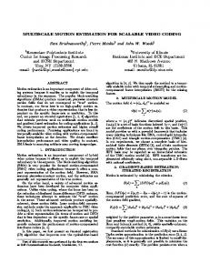
should be translated into a function of X and Y, described as follows. First, the function DIntra (Eq. (4)) should be converted to a continuous-time function. Usually, only a small number of blocks in a non-key frame are with intra mode (NIntra should be small). It can be observed from the curve “Actual” in Fig. 2(a) that in a nonkey frame, the first few blocks in the decreasingly sorted list of motion activities of blocks usually have larger variances, and these variances will decrease as the motion activities decrease. Hence, it is reasonable to model σ i2,Intra as a decreasing linear function: G(t) = A·(1 – t), A > 0, 0 ≤ t ≤ 1, t = i / Nb, 1 ≤ i ≤ NIntra, (8) where A can be derived from the previous PRD optimization result [10]. It can be observed from Fig. 2(a) that when the block index i < 5 (X < 25%) in the total 20 blocks, the function G(t) is accurate enough to model σ i2,Intra . To get the continuous-time version of DIntra in Eq. (4), we let

1

⎛ N Intra ⎞ N Intra and obtain S = ⎜⎜ ∏ σ i2,Intra ⎟⎟ ⎝ i =1 ⎠

ln S =

1

N Intra

N Intra

i =1

∑ (ln σ

2 i , Intra

).

(9)

The continuous-time version of lnS can be written as: Nb ln S = N Intra

N Intra Nb

1

X

∑ ln G(t ) = X ∫ ln[A(1 − t )]dt.

t=

1 Nb

(10)

0

By applying the Taylor expansion to Eq. (10), S can be derived as: −1−

1 (1− X ) ln (1− X ) X

≈ A × (1 − 0.5 × X ) , 0 ≤ X ≤ 1.

(11) Hence, based on Eqs. (4), (9), and (11), DIntra can be derived as: S = A⋅e

DIntra ( X , Y , R ) = A(1 − 0.5 X ) ⋅ 2

R − 2γ X +Y

.

(12)

Second, DInter in Eq. (5) can be expressed as DInter(X, Y, RInter), described as follows. Usually, the variance of the significant pixels for a block with inter mode will decrease as the motion activity decreases. Based on Fig. 2(b), it is reasonable to model σ i2,Inter as a decreasing exponential function as: H (t ) = B1e − B2t , B1 > 0, B2 > 0, 0 ≤ t ≤ 1, t = i / Nb, NIntra + 1 ≤ i ≤ NIntra + NInter, (13) where the parameters B1 and B2 can be derived from the previous PRD optimization result [10]. Actual

Variance 8000 7700 7400 7100 6800 6500 6200 5900 5600 5300 1

2

3

4

5

Actual

Variance 3100 2790 2480 2170 1860 1550 1240 930 620 310 0

Estimated

6

7Block index (i )

1

3

5

7

Estimated

9

11 13 15 17 19 Block index (i )

(a) (b) Fig. 2. (a) The curve “Actual” shows the variances of the first few blocks in the decreasingly sorted list of motion activities of blocks for the Ballroom and Exit sequences. All the variances for the same block index in each nonkey frame are averaged. The curve “Estimated” shows the linear function G(t). (b) The curve “Actual” shows the variances of the significant pixels in the blocks in the same decreasingly sorted list of (a). The curve “Estimated” shows the function H(t).

To get the continuous-time version of the first term of DInter in Eq. 1

(5), by letting

⎛ N Intra + N Inter ⎞ N Inter , considering the continuousT = ⎜⎜ ∏ σ i2,Inter ⎟⎟ ⎝ i = N Intra +1 ⎠

time version of lnT, and applying the similar approximation technique, T can be approximated as: (14) T ≈ B1 × h( X , Y ) , 0 ≤ X, Y ≤ 1 and X + Y ≤ 1, where h(X, Y) = h1(X)×h2(Y), and (15) h1 ( X ) = (0.5 B22 e −0.3 B )X 2 − B2 e −0.3 B (1 + 0.3B2 )X + e −0.3 B (0.045 B22 + 0.3B2 + 1), −0.2 B −0.2 B 2 −0.2 B 2 2 h2 (Y ) = (0.125 B2 e )Y − B2 e (0.5 + 0.1B2 )Y + e (0.02 B2 + 0.2 B2 + 1) . (16) Similarly, it is reasonable to model δ i2,Inter as a decreasing linear 2

2

2

2

2

2

function:

I(t) = C·(1 – t), C > 0, 0 ≤ t ≤ 1, t = i / Nb, (17) NIntra + 1 ≤ i ≤ NIntra + NIner, where C can be derived from the previous PRD optimization result [10]. By considering the continuous-time version of the second term of Eq. (5) and Eq. (14), DInter can be derived as: − 2γ

R

DInter ( X , Y , RInter ) = B1h( X , Y ) ⋅ 2 X +Y + C (1 − X − 0.5Y ) . (18) Third, DSkip in Eq. (6) can be derived as follows. By considering the inverse order of the decreasingly sorted list of motion activities of blocks, as the motion activity increases, the MSE of a block with skip mode will increase. It is reasonable to model δ i2,Skip as an increasing exponential function as: K (t ) = D1e D2t , D1 > 0, D2 > 0, 0 ≤ t ≤ 1, (19) t = i / Nb, 1 ≤ i ≤ NSkip, where D1 and D2 can be derived from the previous PRD optimization result [10]. By applying the similar approximation technique, DSkip can be approximated as: (20) ( ) D1 ( ( ) ) D Skip Z =

ZD2

k Z −1 ,

where Z = 1 – X – Y, and k (Z ) = (0.5D22 e 0.3 D )Z 2 + D2 e 0.3D (1 − 0.3D2 )Z + e 0.3 D (1 − 0.3D2 + 0.045D22 ) . (21) Finally, based on Eqs. (7), (12), (18), and (20), the overall PRD optimization problem can be formulated as: 2

2

2

min DOverall ( X , Y , R )

{X ,Y }

R R − 2γ −2 γ ⎧ ⎫, = min⎨ A(X − 0.5 X 2 )⋅ 2 X +Y + P( X , Y ) ⋅ 2 X +Y + Q ( X , Y )⎬ {X ,Y } ⎩ ⎭

s.t. F(C1X + C2Y + C3R) ≤ Φ(P), where P( X , Y ) = B1Yh( X , Y ) , and Q ( X , Y ) = CY (1 − X − 0.5Y ) +

D1 [k (1 − X − Y ) − 1]. D2

(22) (23) (24)

Further simplification of Eq. (22) will be investigated in our future work. Here, discrete sampling on X and Y, (X, Y) = (0.05x, 0.05y), x, y = 0, 1, 2, …, 19, under the constraints, 0 ≤ X, Y, X + Y ≤ 1, and Eq. (1), are evaluated to find the optimal (X, Y) in minimizing Eq. (22). The analytic and actual PRD performances for the Ballroom sequence are shown in Fig. 3. 4. SIMULATION RESULTS Two multiview video sequences consisting of 250 frames, a frame size of 640×480, a block size of 128×128 (n = 128), YUV4:0:0 (only luminance component was evaluated), and a frame rate of 10 frames per second (fps) were used to evaluate our low-complexity multiview video codec under different available resources. The four low-complexity video encoder approaches, including our lowcomplexity single-view video codec (Proposed Single) [11], the H.264/AVC intraframe codec (H.264 Intra) [2], the H.264/AVC interframe codec with no motion, where all the motion vectors are set to zeros, with GOP size set to 2 (H.264 No motion (GOP = 2)), and the H.264/AVC interframe coding with no motion with GOP size set to infinity (H.264 No motion (GOP = ∞)) were employed for comparisons with our codec. In this paper, the two metrics, i.e.,

RD performance and encoding complexity, were used for performance evaluation. Φ(P)=0.05 (Estimated) Φ(P)=0.1 (Estimated) Φ(P)=0.5 (Estimated) Φ(P)=0.7 (Estimated) Φ(P)=1.0 (Estimated)

MSE

Φ(P)=0.05 (Actual) Φ(P)=0.1 (Actual) Φ(P)=0.5 (Actual) Φ(P)=0.7(Actual) Φ(P)=1.0 (Actual)

Average encoding time (sec) 3.3

2.4 2.1 1.8 0

0.2

0.3

0.4

0.5

0.6

0.7

0.8

0.9

1 R (bpp)

The average PRD performances for the three adjacent VSNs listed in Table 1 are shown in Fig. 4(a) and (b), respectively, for the Ballroom and Exit sequences. For the Ballroom sequence, it can be observed from Fig. 4(a) that the PSNR performance gains of our multiview video codec at Φ(P) = 1.0 above those of the H.264 No motion are from 0.1 to 4 dB. The PSNR performance gains of our multiview codec at Φ(P) = 1.0 above those of the H.264 Intra are from 2 to 6 dB. The RD performance of our codec at Φ(P) = 0.5 is very close to that of our codec at Φ(P) = 1.0, especially at higher bit rates. The RD performance of our codec at Φ(P) = 0.05 is very poor. The PSNR performance gains of our codec at higher powers can significantly outperform our singleview codec. Similar results can also be observed from Fig. 4(b) for the Exit sequence. More specifically, our codec can outperform the three approaches used for comparisons, especially at high power and low bit rates. That is, when the power is high, our encoder can efficiently exploit the available bit rates to optimize the video quality, even though the bit rate is low. In addition, with the benefits of exploiting the reference frames from the adjacent view, our encoder can have more skipped SDS symbols or skipped blocks, which can save more bit rates. Proposed (Φ(P) = 1.0) Proposed (Φ(P) = 0.1) H.264 No motion (GOP = ∞) H.264 Intra (GOP = 1)

Proposed (Φ(P) = 0.5) Proposed Single H.264 No motion (GOP = 2)

PSNR (dB) 40

38

38

36

36

34

34

32

32

30

30

28

Proposed (Φ(P) = 1.0) Proposed (Φ(P) = 0.1) H.264 No motion (GOP = ∞) H.264 Intra (GOP = 1)

Proposed (Φ(P) = 0.5) Proposed Single H.264 No motion (GOP = 2)

28

26

26 100

200

300

400

200

400

600

800

1000 Bitrate (kbps)

Fig. 5. The average encoding time per frame for the Ballroom sequence.

Fig. 3. The curves “Estimated” show the PRD performance obtained from our PRD model, whereas the curves “Actual” show the actual PRD performance obtained from our video codec for the Ballroom sequence.

0

Proposed (Φ(P) = 0.5) H.264 No motion (GOP = 2)

2.7

0.1

40

Proposed (Φ(P) = 1.0) H.264 No motion (GOP = ∞) H.264 Intra (GOP = 1)

3.0

330 300 270 240 210 180 150 120 90 60 30 0

PSNR (dB)

our codec is lower than those of the three H.264/AVC lowcomplexity codecs, even though when the full power is applied.

500

600

700

800

900 1000 Bitrate (kbps)

0

100

200

300

400

500

600

700

800

900 1000 Bitrate (kbps)

Fig. 4. The RD performances for the (a) Ballroom, and (b) Exit sequences.

Although it is claimed that the proposed codec and the existing codecs used for comparisons are all with low-complexity encoder, it is still important to compare their encoding complexities. The respective average encoding time per frame for the Ballroom sequence of the evaluated codecs, measured on a Pentium-4 PC with 3.40GHz CPU and 1.49GB RAM at different bit rates is shown in Fig. 5. The encoding time of the proposed codec includes the time consumed in interview hash data exchanges, where the hash data size is relatively small (e.g., average 3.78 kbit, i.e., about 0.16% of the original frame size, per frame). By considering the typical data transmission rate, 40 kbps, for a common sensor node [1] (actually, the rate may be higher for a VSN, e.g., 250 kbps [1] or 1 Mbps [6]), it takes only 0.09 seconds to achieve hash data exchange per frame. Fig. 5 shows that the encoding complexity of

5. CONCLUSIONS In this paper, we have proposed a PRD model to characterize the relationship between the available resources and the RD performance of our low-complexity multiview video codec. Based on this model, the resource allocation can be efficiently performed at the encoder while optimizing the reconstructed video quality. Analytic results have been provided to verify the resource scalability and accuracy of the proposed PRD model. For future work, the distortion induced by wireless video transmission will be integrated into the current distortion function to form a complete end-to-end distortion function. More precise theoretical analyses, such as the optimal achievable video quality based on available resources and the minimum resource requirements based on acceptable video distortion, need to be derived to provide a practical guideline in preparation and deployment for a WVSN. ACKNOWLEDGEMENT This work was supported in part by National Science Council, Taiwan, ROC, under Grants NSC95-2422-H-001-031 and NSC 95-2221-E-001-022. REFERENCES [1] I. F. Akyildiz, T. Melodia, and K. R. Chowdhury, “A survey on wireless multimedia sensor networks,” Computer Networks, 2007. [2] T. Wiegand and G. J. Sullivan, “The H.264/AVC video coding standard,” IEEE Signal Processing Mag., vol. 24, pp. 148-153, 2007. [3] A. Smolic et al., “Coding algorithms for 3DTV-a survey,” IEEE Trans. on Circuits and Sys. for Video Tech., vol. 17, pp. 1606-1621, 2007. [4] C. Guillemot et al., “Distributed monoview and multiview video coding: basics, problems and recent advances,” IEEE Signal Processing Magazine, vol. 24, no. 5, pp. 67-76, Sept. 2007. [5] X. Guo et al., “Wyner-Ziv-based multi-view video coding,” IEEE Trans. on Circuits and Sys. for Video Tech., vol. 18, 2008. [6] M. Wu and C. W. Chen, “Collaborative image coding and transmission over wireless sensor networks,” J. Advances Signal Process., 2007. [7] Z. He and D. Wu, “Resource allocation and performance analysis of wireless video sensors,” IEEE Trans. on Circuits and Systems for Video Technology, vol. 16, no. 5, pp. 590-599, May 2006. [8] L. W. Kang and C. S. Lu, “Multi-view distributed video coding with low-complexity inter-sensor communication over wireless video sensor networks,” Proc. IEEE Int. Conf. on Image Processing, Sept. 2007. [9] C. S. Lu and H. Y. M. Liao, “Structural digital signature for image authentication: an incidental distortion resistant scheme,” IEEE Trans. on Multimedia, vol. 5, no. 2, pp. 161-173, June 2003. [10] L. W. Kang and C. S. Lu, “Power-rate-distortion optimized resource allocation for low-complexity multiview distributed video coding,” TR-IIS-08-003, IIS Technical Report, Institute of Information Science, Academia Sinica, 2008. [11] L. W. Kang and C. S. Lu, “Low-complexity Wyner-Ziv video coding based on robust media hashing,” Proc. IEEE MMSP, Oct. 2006.