arXiv:quant-ph/0205001v1 30 Apr 2002. Power series Schrodinger ..... Some representative (un-normalized) wave functions. Only the larger coefficients are.
Power series Schrodinger eigenfunctions for a particle on the torus.
arXiv:quant-ph/0205001v1 30 Apr 2002
Mario Encinosa and Babak Etemadi Department of Physics Florida A & M University Tallahassee, Florida 32307 Abstract The eigenvalues and a series representation of the eigenfunctions of the Schrodinger equation for a particle on the surface of a torus are derived. Introduction. The eigenvalues and eigenfunctions of the Schrodinger equation for a particle constrained to a ring are derived in undergraduate quantum mechanics textbooks as examples of quantization from periodic boundary conditions [1]. One might expect that finding the eigenfunctions Ψ for the problem of a particle on a toroidal surface with (∇2 + k 2 )Ψ = 0
(1)
would follow simply from similar considerations, and, perhaps, even foolishly claim this to be true while lecturing to one’s math methods students. A Google search on ”torus quantum eigenfunctions” returns many links to esoterica in compactification, chaotic maps and plasma dynamics. Here we address a more prosaic textbook type problem: finding the eigenvalues and eigenfunctions (to the best of our knowledge there are no closed form solutions) of the Schrodinger equation for a particle on the surface of a torus. Solution Method. Toroidal coordinates [2] are defined through the relations x=
c sinhα cosφ coshα − cosβ
(2a)
y=
c sinhα sinφ coshα − cosβ
(2b)
z=
c sinβ . coshα − cosβ
(2c)
A simple substitution renders Laplace’s equation separable in (α, β, φ), yielding solutions in terms of non-integer Legendre functions [3]. This suggests that the eigenvalue problem could be solved by examining the limiting case of two toroidal shells or by setting α, the coordinate that loosely speaking acts as the ”radial” coordinate in the system given by equations [2a-2c] to a fixed value. Unfortunately for the former choice, the presence of the energy term on the right hand side of Schrodinger’s equation precludes the substitution
that leads to separability. The latter option gives a differential equation that can be solved by the methods employed below, but here we choose to use a more intuitive parametric representation defined by x = (R + a sinθ) cosφ (3a) y = (R + a sinθ) sinφ
(3b)
z = a cosθ.
(3c)
We assume the simplest possible choice for the Hamiltonian, H = − 12 ∇2 , and take for ∇2 [4] � � 1 2 − 12 ∂ ij ∂ 2 ∇ =g g g . (4) ∂q i ∂q j A straightforward calculation gives
so that
ds2 = a2 dθ 2 + [R + a sin θ]2 dφ2 ,
(5)
� � cos θ ∂ 1 ∂2 1 1 ∂2 + + . H =− 2 a2 ∂θ 2 a[R + a sin θ] ∂θ [R + a sin θ]2 ∂φ2
(6)
Making the standard ansatz for the azimuthal eigenfunction χ(φ) = exp [imφ], and defining a , β = 2Ea2 , gives for equation (6) α= R ∂ 2ψ α cos θ ∂ψ m2 α2 + − ψ + βψ = 0. ∂θ 2 [1 + α sin θ] ∂θ [1 + α sin θ]2
(7)
Equation (7) appears somewhat similar to several well known equations from SturmLiouville theory [5], and as such, suggests a substitution of the form x = sinθ. That this sort of substitution is untenable becomes clear when it is noted that θ runs over [0, 2π]; x = sinθ can not cover the entire angular range on the torus. Instead, since ψ(θ) must satisfy ψ(θ+2π) = ψ(θ), we choose to expand the solution in Fourier series with z = exp [iθ] as ∞ X ψ(z) = cn z n . (8) n=−∞
The Hamiltonian given by equation (7) is invariant under θ → π − θ, so the solutions of equation (7) can be split into odd and even parity eigenfunctions. For the Fourier expansion given by equation (8) this results in even parity → c0 = arbitrary, cn = (−1)n c−n
(9)
odd parity → c0 = 0, cn = (−1)n+1 c−n .
(10)
We consider first the m = 0 solutions; these cases illustrate the general approach ∂ ∂ → ∂z without the complications that ensue when m 6=0. Letting ∂θ ∂θ ∂z in equation (7) gives after some algebra the three term recursion relation [n(n + 1) − β]cn+1 +
2i (β − n2 )cn + [β − n(n + 1)]cn−1 = 0. α
(11)
The n = 0 case of equation (11) gives c1 =
2i c0 α
(12)
for the positive parity solutions and c−1 = c1
(13)
for the negative parity solutions. The recursion relation given by equation (11) approaches some fixed constant at large n, hence will diverge for arbitrary z. However, unlike that which occurs for standard issue two term recursion relations [4], there is no way to force all higher order coefficients to zero. To make the series convergent requires more work. Consider the positive parity coefficient cN ; the numerator of cN will be a polynomial of degree N − 1 in β, with N − 1 roots. The numerator of cN+1 with be a polynomial of degree N obtained from multiplication of cN by a factor of (β − n2 ) and addition of a lower order polynomial in β. Suppose the lower order cN numerator is factored into its roots as ). cN ≈ (β − λ1N )(β − λ2N )...(β − λN−1 N
(14)
cN+1 ∼ (β − N 2 )(β − λ1N )(β − λ2N )...(β − λN N ) + F (β)
(15)
≡ (β − λ1N+1 )(β − λ2N+1 )...(β − λN N+1 ),
(16)
Then
so that given the roots of the N th order polynomial they can serve as test roots for the (N + 1)th . In practice the lower order roots converge very quickly, and, as n increases the roots quickly approach the n2 limit. Once the roots are determined to a given order, they can be fed back into the lower order terms and the series safely truncated at order N + 1. c0 can then be adjusted to whatever boundary value desired (results will be presented in the next section). For m 6= 0, equation (7) gives a five term recursion relation �
� � � α α2 n αin α2 2 2 cn−2 + cn−1 + [β − (n − 2) ] + [β − (n − 1) ] + − 4 4 i 2
� � α2 2 2 2 2 )(β − n ) − m α cn + (1 + 2 � � � � α2 αin αn α 2 2 cn+1 + − cn+2 = 0. [β − (n + 2) ] − − [β − (n + 1) ] + i 2 4 4
(16)
The three lowest coefficients of the positive parity solutions must obey [(1 +
1 α2 α2 2 )β − m2 α2 ]c0 + 2iα(β − )c1 + c2 = 0. 2 2 2
(17)
The recursion relation involving the lowest coefficients of the negative parity solutions gives 0 = 0, so for both cases there are no restrictions on the two lowest coefficients. The full solution for either parity must be some linear combination of two linear independent solutions. Again consider the positive parity case (the procedure is of course identical for the negative parity solutions). To generate two linearly independent solutions, say ψA and A B B ψB , convenient choices are (cA 0 ,c1 ) = (1, 1) and (c0 , c1 ) = (1, −1). Each choice in turn will generate series in β, and the total solution will be some linear combination of the two series. To determine eigenvalues and the proper linear combination, insist that at some large value of n, say N , B AcA (18a) N + BcN = 0 B AcA N+1 + BcN+1 = 0.
(18b)
The homogenous pair of equations (18a,18b) have nontrivial solutions only when the determinant of the c matrix vanishes. The zeros of the determinant are the eigenvalues. The ratio of B to A can be determined for each eigenvalue by reinsertion of the eigenvalue into equations (18a) and (18b), and A (or B) then fixed by an initial condition. The procedure just described will work for m = 0 states also. Results. In table 1 we show m = 0 eigenvalues Eλ0 for low lying states as determined by the power series method in comparison to a Runge-Kutta solution of equation (7) (α = .5 for all results). The differential equation is solved by choosing ψ(− π2 ) = 1(0) and ψ ′ (− π2 ) = 0(1), . Either integrating forward to π2 , then integrating from - π2 in the lower half plane to − 3π 2 ′ ψ (for negative parity) or ψ (for positive parity) for both integration paths must vanish at π . It is clear that at least for low lying states, convergence to a good number of decimal 2 places is obtained. Tables 2 and 3 show some m = 1 and m = 5 eigenvalues. Table 4 shows a comparison between power series values and values obtained by solving equation (7) numerically. The values indicated in table 4 are the result of summing to n = 6 which gave at least four digits of accuracy with the differential equation solution, although fewer than six is usually sufficient. Finally, table 5 gives a few normalized wave functions. ψ22 was listed specifically to show its resemblance to ψ10 ; it is the next to lowest eigenvalue of the m = 2 state, but has qualitatively the same character as the m = 0 ground state. This is a topic currently under investigation. Conclusions. We have shown that a Fourier series method can be used to determine eigenvalues and eigenfunctions of (at least one version) of the Schrodinger equation for a particle that lives on the surface of a torus. This work was initially motivated by investigations into two other areas: constrained quantum mechanics [6,7,8] and carbon nanotube physics [9,10]. In both areas it proved necessary to determine surface wave functions for low-lying states, and to our surprise, analytic forms were not to be found. Because of the importance of toroidal geometry in so many branches of physics, it is curious that if closed form eigenfunctions exist (in the sense
that they could be looked up in the standard references), they do not appear in textbooks. Should the closed form solutions be known, their publication would certainly provide both a useful pedagogical and practical research tool.
Acknowledgments The authors would like to acknowledge useful discussions with Mr. Lonnie Mott. M.E. received support from NASA, NAG2-1439.
References 1. A. Goswami, Quantum mechancs, (Wm. C. Brown, Dubuque, 1992). 2. http://mathworld.wolfram.com/ToroidalCoordinates.html 3. J. Vanderlinde, Classical electromagnetic theory (J. Wiley and Sons, New York, 1993). 4.G. Arfken and H. Weber,Mathematical methods for physicists, 4th ed., (Academic Press, New York, 1995). 5. S. Ross,Differential equations, 2nd ed., (J. Wiley and Sons, New York, 1974). 6. R. C. T. da Costa, Phys. Rev. A 23, 1982 (1981). 7. L.Kaplan, N.T. Maitra and E.J. Heller, Phys. Rev. A, 56, 2592 (1992). 8. M. Encinosa and R.H. O’Neal, quant-ph/9908087. 9. H.R. Shea, R. Martel, Ph. Avouris, Phys. Rev. Lett. 84, 4441 (2000). 10. M. Sano, A. Kamino, J. Okkamura and S. Shinkai, Science, 293 1299 (2001).
Table 1 E1 E2 E3
N=3 1.134245 4.242039 *******
N=5 1.122415 4.054351 9.077862
N=10 1.122288 4.051724 9.041071
DE 1.122286 4.051722 9.041070
Low lying m = 0 eigenvalues from roots of cN , Fourier coefficient of ψ(θ). The eigenvalue for the differential equation (DE) solution was truncated when continuity of order ∼ 10−7 in ψ(θ) or ψ ′ (θ) (see text) was obtained. Asterisks indicate a root does not appear at that order. Table 2 N E1 E2 E3
N=3 .247927 1.658615 *******
N=5 .249375 1.662639 4.485872
N=10 .249368 1.663015 4.476692
DE .249368 1.663015 4.476693
Low lying m = 1 eigenvalues as roots of the cN coefficient of the Fourier expansion for ψ(θ). Table 3 N E1 E2 E3
N=3 3.732776 ******* 14.771896
N=5 3.705405 8.855027 15.289127
N=10 3.705427 8.853639 15.164616
DE 3.705428 8.853640 15.164615
Low lying m = 5 eigenvalues. The appearance of a larger root before a smaller root is not unusual for higher m values. Table 4 θ ψF S ψDE
− π3 .908836 .908780
− π4 .796182 .796192
0 .270886 .270874
π 6
-.105468 -.105471
π 2
-.479280 -.479273
ψ21 (θ) from the Fourier series expansion compared to the differential equation solution. Table 5 ψ10 =.1853 - .7413 sinθ + .0608 cos2θ ψ22 =.2667 - .7425 sinθ + .0052 cos2θ ψ31 =.2671 -.5409 sinθ - .4886 cos2θ - .2794 sin3θ Some representative (un-normalized) wave functions. Only the larger coefficients are shown; all others are an order of magnitude less than those given.