1248
IEEE TRANSACTIONS ON POWER SYSTEMS, VOL. 18, NO. 4, NOVEMBER 2003
A New Preconditioned Conjugate Gradient Power Flow Hasan Dag, Member, IEEE, and Adam Semlyen, Life Fellow, IEEE
Abstract—A new solution methodology for the constant matrix, decoupled power flow problem is presented in this paper. The proposed method uses the conjugate gradient method instead of the for updating the power flow traditional direct solution of variables. The conjugate gradient method is accelerated with an approximate inverse matrix preconditioner obtained from a linear combination of matrix-valued Chebyshev polynomials. The new method has been tested on several systems of different sizes. In terms of speed, the method is comparable to the fast decoupled load flow [1] in serial environments but it is more amenable to parallel and vector processing since it contains only matrix-vector multiplications.
=
Index Terms—Chebyshev polynomials, conjugate gradient method, decoupled load flow, iterative methods, preconditioner.
I. INTRODUCTION
T
HE solution of the power flow problem has been extensively studied over the last four decades and still attracts many researches to the field. A current topic of interest has been the application of iterative solvers for the solution of the linear equations (1a) (1b) in the fast decoupled load flow (FDLF) [1] iterations and for the solution of (2) in the Newton-Raphson load flow. Both (1) and (2) represent only one step of the power flow problem and are traditionally solved by a direct method with sparsity technique [2]. The coand are computed and factorized once efficient matrices [1], while the Jacobian matrix is recalculated and refactorized for each Newton-Raphson iteration. and this notation Equations (1) and (2) are of the form will be used for the rest of the paper. The application of iterative Manuscript received May 9, 2001; revised April 14, 2002. This work was supported by the Natural Sciences and Engineering Research Council of Canada. The work has been done during H. Dag’s leave in the summer of 1997 to conduct research at the University of Toronto, ON, Canada. H. Dag is with the Department of Electrical Engineering of the Istanbul Technical University, Maslak, Istanbul 80626, Turkey (e-mail:
[email protected]). A. Semlyen is with the Department of Electrical and Computer Engineering of the University of Toronto, ON M5S 3G4, Canada (e-mail:
[email protected]). Digital Object Identifier 10.1109/TPWRS.2003.814855
methods to power system problems, specifically to the power flow solutions has, in general, two variants. One variant is the formulations where the linear system of equations has a symmetric, positive definite coefficient matrix, and the other one is the formulations with nonsymmetric, possibly indefinite, linear systems. Equation (1) and the dc load flow can be given as examples for the former, and (2) for the latter [3]. For symmetric, positive definite linear systems, a good choice of iterative solution is the conjugate gradient method (CGM) [4], [5]; see Appendix A. For nonsymmetric linear systems, there are many variants one can choose. Since this paper deals with the former, the nonsymmetric formulation of the power flow problem will not be pursued further. However, the interested reader is referred to [6] for the whole class of nonsymmetric iterative methods and to [7]–[9] for the application of nonsymmetric iterative methods to the power flow problem. It has been reported that the use of CGM for power flow solutions decreases the computation time, relative to the LDU factorization based direct methods, for large power system problems [10], [11]. In these studies, an incomplete LU (ILU) factorization of the coefficient matrix of the linear system is used to accelerate CGM. However, in order to increase the effectiveness of the acceleration (called preconditioning), the matrix needs to be reordered. This is due to the fact that the error between the full LU factors and ILU after ordering will be smaller than before ordering. Several studies [12], [13] have confirmed that ordering affects both the rate of convergence of CGM and the number of conjugate gradient (CG) iterations. ILU as a preconditioner is quite effective in clustering the eigenvalues of the linear system. However, it has to be recalculated if there are structural changes in the network, such as double line outage in contingency analysis and bus-type switching during the solution of the power flow problem. Also, the ILU preconditioner is not amenable to parallel processing due to the sequential nature of forward and back substitutions. This paper describes a new type of preconditioner, an approximate inverse of the coefficient matrix of the linear equations to be solved. It is obtained from a linear combination of matrix-valued Chebyshev polynomials. The preconditioner does not need matrix ordering and its calculation requires only a few matrix vector multiplications to estimate the largest eigenvalue of the linear equations, and a shifting of the coefficient matrix. We also investigate the effect of premature termination of the CG solution of linear equations on the power flow iterations. These will be referred to as external iterations in the rest of the paper to distinguish them from the CG iterations.
0885-8950/03$17.00 © 2003 IEEE
DAG AND SEMLYEN: A NEW PRECONDITIONED CONJUGATE GRADIENT POWER FLOW
1249
In the following, first the scalar-valued Chebyshev polynomials are introduced and a statistical study of approximating inverses of scalars with these polynomials is performed. Then, a correlation of this study to matrix inverse approximation is given. The approximate inverse of the matrix will then be used as preconditioner to accelerate the CGM when solving (1a) and (1b). II. THEORETICAL BASIS A. Motivation Those who have applied iterative methods to power system problems have indicated the need for a better preconditioner, possibly taking the physical structure of power systems into account. Better could mean the following: • easy to obtain and easy to apply; • be good at clustering the eigenvalues of the original linear system at hand so that CGM takes fewer iterations; • be amenable to parallel processing; • the cost of computing the preconditioner is minimal. So far, there is not a single preconditioner that possesses all of these desirable features. The traditional ILU preconditioner is very good in terms of the second characteristic but it is not amenable to parallel processing and requires matrix ordering. The goal of this paper is to present a preconditioner that possesses all of the aforementioned features.
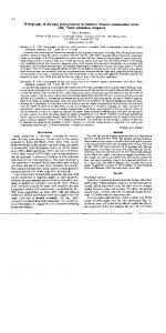
Fig. 1.
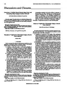
Some Chebyshev polynomials T (z) up to order 8.
B. Chebyshev Preconditioner In this section, we develop the proposed preconditioner. To this end, it will be useful to first introduce the scalar-valued Chebyshev polynomials. These orthogonal polynomials can be calculated recursively using the following relations: (3a) (3b) Fig. 1 shows Chebyshev polynomials of different orders. The , in fact, they polynomials have the property that and 1 on the domain . oscillate between , can The inverse of scalar numbers , where be computed from a linear combination of these polynomials using the convergent series (4) shifts the values of where into the interval . The coefficients in (4) for the inare calculated from the relations below (see[14, terval page 357])
(5)
Equation (4) computes the inverse of scalars exactly. However, an approximate inverse of any scalar in the above interval can be computed using a linear combination of the scalar-valued
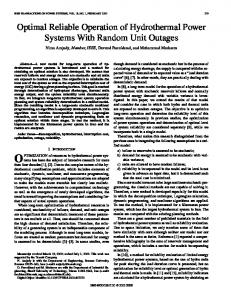
Fig. 2. Error in approximating a scalar inverse using a linear combination of Chebyshev polynomials.
Chebyshev polynomials of small order. The use of a linear combination of the Chebyshev polynomials of different orders to obtain the approximate inverse of scalars is illustrated in Fig. 2. means obtaining the inverse of from a In Fig. 2, Cheb linear combination of the scalar-valued Chebyshev polynomials of degree up to . As can be seen from the figure, for a small range of scalars (the top left subplot), a good approximate inverse is obtained from a linear combination of the polynomials of degree up to 3. The deviation from unity of the product of scalars and their approximate inverses is less than 25% (top right subplot). If the order of the polynomial is increased, the approximation, as expected, gets better and the deviation becomes less than 2% (middle subplots). However, as the range of numbers is increased, the approximate inverse, even with polynomials up to order seven, is not good. The deviation can become as big as 2000% (bottom subplots). From here on, we will call condition number the ratio of the largest number to the smallest number . in the range and denote it as
1250
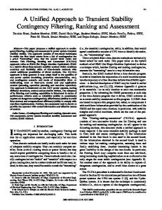
Fig. 3. Deviation (y 3 Cheb(y)-1) in approximating the inverse of scalar numbers using Chebyshev polynomials up to order 25.
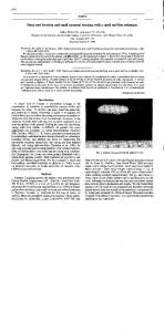
Fig. 3 shows the scalar inverse approximation for larger intervals of scalars (large condition numbers) using Chebyshev polynomials up to order 25. The deviations form a smooth surface. As expected, using higher order polynomials reduces the deviation substantially. Nonetheless, for very big condition numbers, 10 000 or more, even the linear combination of polynomials up to order 25 gives a very big deviation. Our goal is to approximate the inverse of a matrix , whose . Then, and are the spectrum is contained in the interval smallest and the largest eigenvalues of , respectively. The errors resulting from the scalar inverse approximation in the interval can be used to predict the error in approximating the inverse of . This is due to the fact that any action of a matrix as an operator can be fully characterized by its eigenvalues. This justifies our focusing on the scalar inverses. (For a proof, see Appendix B). From Figs. 2 and 3, it can be seen that the deviation is worse at the right end of the interval. That is, the approximate inverse of scalars near have much larger deviation than those near the smallest scalar in the interval. The question that now arises is whether there is a way of reducing the deviation where it is big, at the expense of increasing it, hopefully just slightly, where it is small, so that the overall deviation becomes smaller. The term artificial conditioning will be used to indicate moving toward . That is, we are still interested in finding the approximate in, but in (5) instead of the verses of scalars in the interval . Now the ratio original we use a larger value, will be termed the artificial condition number. For example, if , then the artificial condition number is 25. Fig. 4 shows the effect of moving toward (artificial conditioning) for scalars between 1 and 100. Note that as the artificial condition number is made smaller, the deviation at the right end of the range of numbers gets smaller, but the deviation at the left end does not become worse than its initial value, the deviation . The immediate conclusion from this observation is at , that when approximating scalar inverses in the interval does not have to be set to the first scalar in the interval as implied by (5). The question Fig. 4 raises is how small the artificial
IEEE TRANSACTIONS ON POWER SYSTEMS, VOL. 18, NO. 4, NOVEMBER 2003
Fig. 4. Effect of artificial conditioning in approximating inverses of scalars between 1 and 100.
condition number can be made. In other words, does there exist an optimal artificial condition number (in the sense of smallest deviation)? To answer the above question, we conducted a statistical study of the artificial conditioning for various condition numbers for both linearly and logarithmically spaced scalars. The reason for choosing such scalar distributions is due to the distribution of eigenvalues of power system matrices exhibiting a logarithmic-looking spectrum. For each condition to , we generated 2000 scalars number ranging from and approximated their inverses using (4) with Chebyshev polynomials of various orders. Ideally, the product of a scalar and its inverse is 1. However, when the polynomials are of small order, the inverse will only be approximate. In order to find an optimal value for the artificial condition number, the ratio of the standard deviation and the mean of the product of the scalars and their approximate inverses are computed. The ratio that results in a minimum (which indicates the best statistical distribution of the product around unity) is the optimal artificial condition number for both the particular range of scalars and the polynomial order. The conclusions of this study are • for logarithmically distributed scalars, the value of the best artificial condition number is five times the maximum polynomial order used in approximating the inverse; • for the linearly distributed scalars, the value of the best indicating the closest artificial condition number, with smaller integer, is . For example, the optimal artificial condition number for logarithmically distributed scalars when using polynomials up to . Similarly, the optimal order 3 is 15. Thus, the value of is value for linearly distributed scalars with the same polynomial . The overall conclusion from the study of order gives artificial conditioning is that when approximating the inverse of while is set to the largest eigenvalue A, can be set to of .
DAG AND SEMLYEN: A NEW PRECONDITIONED CONJUGATE GRADIENT POWER FLOW
1251
The purpose of preconditioning is to improve the condition number of the linear system (see Appendix A) so that CGM converges faster. However, while the condition number gives only a pessimistic upper bound on the convergence rate, the distribution of the eigenvalues is critical for the rate of convergence [5]. The above statistical study is used to obtain the optimal (best compacted) distribution of the eigenvalues of the linear system. Our experience indicates that when the distribution of eigenvalues is optimal, the condition number also assumes a value, which is very close to the optimal condition number attainable with this distribution of eigenvalues. C. Implementation Equation (4) can be rewritten for a matrix , whose spectrum as is in the interval (6) Fig. 5. Effect of scaling and preconditioning.
where (7) and is (an estimate of) the and is the identity matrix. is largest eigenvalue of , which can be computed by the power method. Note that matrix shifts the spectrum of into the in. are the matrix-valued Chebyshev polynoterval and , while the higher order mials with polynomials are computed using (3b) (given for the scalar case). Our intention is to find an approximate inverse of . Hence, the summation in (6) can be stopped at a very small value of [14] (8) is an approximate inverse of and it will be used as a preconin conjunction with ditioner to solve linear equations CGM. The application of the preconditioner matrix can be implemented efficiently. At every CG iteration, a matrix vector , and is a direcmultiplication Gs is required, where tion vector. This multiplication can be done recursively as (9a) (9b) can be computed as a sum of vectors where each term, involves only one new matrix vector multiplication and some vector operations [14].
compacted better when matrices are preconditioned. The diagonal matrix is given by (10) and the scaling is xobtained by (11) matrix of Fig. 5 shows the distribution of eigenvalues of the the IEEE-57 test system for both the scaled and nonscaled cases. and The top left subplot is a histogram of the eigenvalues of . the top right subplot is that of the scaled matrix The bottom subplots show the eigenvalue distribution for the and ). The preconditioner preconditioned matrices ( is the approximate inverse of the respective matrices obtained from a linear combination of the matrix-valued Chebyshev polynomials up to order three inclusive. We note that the eigenvalues are better compacted of the preconditioned-scaled matrix . Scaling than those of the preconditioned nonscaled matrix has two effects • it improves the condition number of the matrix noticeably (see Table II); • the approximate inverse of the scaled matrix with the same order of Chebyshev polynomial has a better eigenvalue compacting effect than for the nonscaled matrix (bottom subplots of Fig. 5).
Thus,
III. EFFECT OF SCALING LINEAR EQUATIONS It has been reported that the scaling of the original linear equations improves the effectiveness (rate of convergence and number of iterations) of CGM [15], [16]. In this paper, we investigate the effect of scaling more closely. As observed earlier, the distribution of eigenvalues of power system matrices is logarithmic-looking. When scaled symmetrically with a diagonal matrix to have unit diagonal entries, the eigenvalues are
IV. TEST RESULTS All simulations were carried out on a Sun workstation using MATLAB version 5.0, which has sparse matrix capability [17]. A simple decoupled load flow program, that does not do any bus switching or control, was used for comparison. The tested networks include IEEE standard test cases (14, 39, 118, and 300 buses), a 216-bus system from EPRI, and some synthesized networks. The synthesized networks were generated by placing smaller systems (14, 39, and 216) on an grid and connecting them by tie lines and by a superimposed high voltage grid. The synthesized networks, when compared
1252
IEEE TRANSACTIONS ON POWER SYSTEMS, VOL. 18, NO. 4, NOVEMBER 2003
TABLE II COMPARISON OF CONDITION NUMBER ESTIMATES
Fig. 6. Comparison of FDLF and Chebyshev preconditioned conjugate gradient (CPCG) load flow. The polynomial order for the Chebyshev preconditioner is 2 and 1 for(1a) and (1b), respectively.
TABLE I COMPARISON OF NUMBER OF EXTERNAL ITERATIONS
with real networks of the same size, behave similarly in terms of matrices and the number the condition number of the and of FDLF iterations for the solution of the load flow problem. The total number of networks tested was 18, the largest with 5400 buses and 8795 branches. In terms of number of flops [floating point operations (e.g., additions and multiplications)], the proposed method is 2–6 times costlier than FDLF. In terms of cpu time, however, they are comparable for large convergence tolerances on power flow mismatches. For example, when a tolerance of 0.1 p.u. in a 100-MVA base is used, the cpu time for both the proposed method and FDLF differ only by about 25% (in favor of FDLF) for the largest network tested. As the convergence tolerance on mismatches is made tighter, the cpu time for FDLF can become up to 50% less than that for the proposed method, but still remains of the same order. This, however, depends largely on the stopping criterion used for CGM and the polynomial order of the Chebyshev preconditioner. In Fig. 6, we present some test results of the comparison of the proposed method and FDLF for different convergence tolerances for the mismatches. The polynomial order for the Chebyshev preconditioner is 2 and 1 for (1a) and (1b), respectively.
The stopping criterion for the CG solution is 0.09. The preconditioner is calculated explicitly since the order of polynomial used was actually small and the matrices are very sparse. As a result, the second power of the matrix does not become much denser. Table I presents the result of a comparative study of the proposed method and FDLF in terms of number of external iterp.u. on 100-MVA ations with a convergence tolerance of base on mismatches for the load flow problem. Both the XB and BX version [18] of the decoupled load flow are used for comparison. The stopping criterion for the Chebyshev Preconditioned . As can be seen Conjugate Gradient (CPCG) method is from the table, the proposed method converges to the solution of the load flow problem in about the same number of external iterations as FDLF. This is so even with a big stopping criterion on CGM (e.g., 0.01). Using such a large tolerance causes CGM to take an oscillating number of iterations to solve the linear equations for each external iteration. For example, it might take three to five iterations to solve the linear (1a) on the first external iteration but it might take 50–60 iterations to solve the same linear equations with a different right-hand side vector (due to mismatch update). Again, on the following external iteration it will take four to five iterations. This oscillation is much smaller in (1b). The problem can be easily corrected, if desired, by using or smaller) stopping tolerance with the cost of intighter ( creasing the total number of CG iterations somewhat. In Table I, the networks of SYN504, SYN1404, and SYN3456 are generated from IEEE-14, IEEE-39, and EPRI-216 original systems, respectively. The table presents only a few cases of the test results, but the conclusions are drawn from all results. As the size of the network becomes larger, the number of external iterations increases slightly. This increase is due to the and matrices, increase in the condition number of the rather than the network size. Experimental tests indicate that the condition number for these matrices ranges from tens to several hundred thousands. Table II shows a comparison of condition number estimates for some of the networks tested. The columns present the condition number estimates for the original matrix , for the preconditioned original matrix , for the scaled , and for the scaled and precondioriginal matrix . The preconditioner is the approximate intioned matrix verse of the respective matrices obtained from a linear combination of the matrix-valued Chebyshev polynomials up to order 2. For the nonscaled matrix, the artificial condition number is 10 and for the scaled matrix it is 5, as the study of artificial conditioning suggested.
DAG AND SEMLYEN: A NEW PRECONDITIONED CONJUGATE GRADIENT POWER FLOW
V. DISCUSSION OF RESULTS AND CONCLUSIONS Today’s power system studies require more and more complex mathematical models due to both power electronic devices applied to the power system for control purposes and to the operation of power systems near their limit [19]. This led the researchers to investigate different solution methodologies and parallel computation for the solution of very large problems. Regarding different methodologies, iterative linear solvers have on occasion shown to be competitive and even faster than conventional direct solvers. On the parallel computation aspect, however, it was soon realized that there are serious limitations in parallelizing the power system problems [20], [21]. The limited parallelization capability is due largely to sequential forward and back substitutions of the direct method and to the need for the ordering of linear equations to minimize factorization fills. The method proposed in the paper contributes to the solution of both problems above. It does not employ substitution and does not require matrix ordering. It is only slightly slower than the direct method in serial environment. However, since it only involves matrix-vector multiplications and vector operations such as inner product, vector update, etc., it is conducive to parallel and vector processing. Consequently, the proposed method is expected to be a better alternative to both the iterative methods that use ILU-type preconditioners, and the direct methods, for high performance computing of very large power system problems. Some salient features of the proposed preconditioner are • Unlike traditional ILU, the proposed preconditioner does not require matrix ordering and symmetry is preserved. • The preconditioner is amenable to parallel processing since its application requires only matrix-vector products. • The preconditioner compacts eigenvalues well even with very small polynomial orders, such as 1 and 2. The proposed algorithm presented in Appendix C, and the contributions of the paper can be summarized as follows: • An effective, simple polynomial preconditioner is proposed and its performance in compacting eigenvalues of linear system is optimized. • The eigenvalue compacting effect of the proposed preconditioner can be easily seen by studying the approximation of inverses of scalars in an interval that contains the eigenvalues of the corresponding matrix. • It is shown that scaling reduces the condition number greatly. In some cases, it reduces it to less than one hundredth of its original value. The eigenvalues of the scaled matrix become better compacted with the proposed preconditioner. • Unlike ILU preconditioner, the proposed preconditioner does not degrade the parallelization of CGM. • The performance of the proposed preconditioner in combination with CGM has been shown to be comparable to FDLF for the solution of the power flow problem in serial environments for a large number of networks. In summary, the main purpose of developing this method is to be able to solve power system problems, which have a symmetric positive definite coefficient matrix, in parallel. Hence, much larger problems can be solved in shorter time. The method
1253
can be used wherever the solution of a set of linear equations of the form is required. If the coefficient matrix is not can instead be positive definite, the linear system solved in parallel. The fast decoupled load flow is a well-established method and most of the time it is good enough for solving moderate-size power flow problems offline. When one needs to monitor a power system online, FDLF may not be fast enough. The new method is not proposed to replace traditional power flow methods for serial environments. It is proposed as an alternative procedure to solve the same or much larger problems in parallel environments. The test results are just to show that the proposed method is comparable to traditional methods and since it does not require ordering and factorization, it is more amenable to parallel processing than FDLF. APPENDIX A A. Conjugate Gradient Method The CGM generates a sequence of vectors that converge to . It mainly requires matrix vector multiplications and vector updates; hence, it is suitable to parallel and vector computation. The sequence of the vectors has the form (A.1) where is an element of Krylov subspace of dimension at most . A Krylov subspace of dimension is defined as (A.2) is the residual vector for the initial guess where for the solution of the linear equations. If the error at step is defined as (A.3) then (A.1) yields (A.4) CGM chooses
in
to minimize (A.5)
This is to say that CGM minimizes the norm of the error at every iteration [4], [5]. The method converges to the exact solution of in at most iterations, where is the dimension of linear system, if exact arithmetic is used. To reduce CGM iterations, it is applied to a linearly transformed form of the system of equations (A.6) (called the preconditioner matrix [14]) is a nonsinwhere . This linear gular matrix chosen such that denotes the contransformation is called preconditioning. dition number of . It is the ratio of its largest and smallest singular values. For a symmetric, positive definite matrix, it is the ratio of the largest and the smallest eigenvalues. A traditional preconditioner is the incomplete LU factors of matrix A [22], [23]. The ideal preconditioner would be the inverse of matrix
1254
IEEE TRANSACTIONS ON POWER SYSTEMS, VOL. 18, NO. 4, NOVEMBER 2003
A; however, the cost of computing it would be higher than that . of solving APPENDIX B A. Error Analysis of Chebyshev Approximation Of The error in the solution of by approximating the inverse of A using a linear combination of the matrix-valued Chebyshev polynomials is bounded by the maximum error in approximating the inverses of scalars in the interval that is determined by the spectrum of A using the scalar-valued Chebyshev polynomials. To show this, recall that any symmetric matrix has linearly is independent eigenvectors. The exact solution of (B.1) The vector can be written in terms of the eigenvectors as
of
• Set and (or ). If , . set • Scale both matrices using (10) and (11), and save the scaling for the and matrices, respectively. matrices and • Use (5) to compute the coefficients. • If is small (such as 1 or 2), use (8) for the approximate inand matrices that will be input to CPCG. verses of the Otherwise, the preconditioning step needs be done on the fly. • While maximum mismatch tolerance ( , , stopping_criterion); • and update mismatches; • undo scaling on ( , , stopping_criterion); • and update mismatches. • undo scaling on In the above algorithm, CPCG(.) is the Chebyshev Preconditioned Conjugate Gradient method. It returns the solution of linear equations when supplied with , , and a stopping tolerance on CG iterations. REFERENCES
(B.2) where
are scalars. Thus, (B.1) can be rewritten as (B.3)
are the eigenvalues of . When approximating the where inverse of using a linear combinations of the matrix-valued Chebyshev polynomials, if the eigenvalues are in error (i.e., ), then (B.4) If the errors are bounded (i.e.,
), then (B.5)
To provide a numerical example for the above proof, let us matrix of the IEEE-14 bus test system with a random take the right-hand side vector as the linear set of equations. When approximating the inverses of the scalars in the interval deterusing a linear combination of the mined by the spectrum of scalar-valued Chebyshev polynomials up to order 5, the maximum scalar deviation is 1.09, and the maximum deviation on the inverses of eigenvalues is 1.06. The maximum error between the true solution and the approximate solution of the linear equations is 1.03. The approximate inverse is obtained using (8) with Chebyshev polynomial order 5. APPENDIX C A. Algorithm for the Proposed Method and matrices (either XB or BX version). • Compute the • Choose a flat start, polynomial order for the Chebyshev preconditioner, and a stopping criterion for CGM.
[1] B. Stott and O. Alsac, “Fast decoupled load flow,” IEEE Trans. Power Apparat. Syst., vol. PAS-93, pp. 859–869, May/June 1974. [2] W. F. Tinney and J. W. Walker, “Direct solutions of sparse network equations by optimally ordered triangular factorization,” Proc. IEEE, vol. 9, pp. 1801–1809, Nov. 1967. [3] H. Dag and F. L. Alvarado, “Toward improved uses of the conjugate gradient method for power system applications,” IEEE Trans. Power Syst., vol. 12, pp. 1306–1314, Aug. 1997. [4] M. R. Hestenes and E. Stiefel, “Methods of conjugate gradients for solving linear systems,” J. Res. Natl. Bur. Stand., vol. 49, pp. 409–436, 1952. [5] J. R. Shewchuk, An Introduction to the Conjugate Gradient Method Without the Agonizing Pain. Pittsburgh, PA: School of Computer Science, Carnegie Mellon University, 1994. [6] R. Freund, G. Golub, and N. Nachtigal, “Iterative solution of linear systems,” in Acta Numerica. Cambridge, U.K.: Cambridge Univ. Press, 1991, pp. 57–100. [7] A. Semlyen, “Fundamental concepts of krylov subspace power flow methodology,” IEEE Trans. Powers Syst., vol. 11, pp. 1528–1537, Aug. 1996. [8] R. Bacher and E. Bullinger, “Application of nonstationary iterative methods to an exact newton-raphson solution process for power flow equations,” in Proc. 12th Power Syst. Comput. Conf., Aug. 19–23, 1996, pp. 453–459. [9] A. J. Flueck and H. D. Chiang, “Solving the nonlinear power flow equations with an inexact newton method using GMRES,” in IEEE/Power Eng. Soc. Winter Meeting, Tampa, FL, Feb. 1–5, 1998. [10] F. D. Galiana, H. Javidi, and S. McFee, “On the application of a preconditioned conjugate gradient algorithm to power network analysis,” IEEE Trans. Power Syst., vol. 9, pp. 629–636, May 1994. [11] H. Mori, H. Tanaka, and J. Kanno, “A preconditioned fast decoupled power flow method for contingency screening,” IEEE Trans. Power Syst., vol. 11, pp. 357–363, Feb. 1996. [12] H. Dag and F. L. Alvarado, “The effect of ordering on the preconditioned conjugate gradient method for power system applications,” in Proc. North Amer. Power Symp., Manhattan, KS, Sept. 26–27, 1994, pp. 202–209. [13] A. B. Alves, E. N. Asada, and A. Monticelli, “Critical evaluation of direct and iterative methods for solving Ax b systems in power flow calculations and contingency analysis,” in IEEE/Power Eng. Soc. Summer Meeting, Berlin, Germany, July 20–24, 1997. [14] O. Axelsson, Iterative Solution Methods. Cambridge, U.K.: Cambridge Univ. Press, 1994. [15] H. Javidi, S. McFee, and F. D. Galiana, “Investigation of eigenvalue clustering by modified incomplete cholesky decomposition in power network matrices,” in Proc. Power Syst. Comput. Conf., Avignon, France, Aug. 1993. [16] H. Dag and F. L. Alvarado, “Direct methods versus GMRES and PCG for power flow problems,” in Proc. North Amer. Power Symp., Washington, D.C., 1993, pp. 274–278.
=
DAG AND SEMLYEN: A NEW PRECONDITIONED CONJUGATE GRADIENT POWER FLOW
[17] J. R. Gilbert, C. Moler, and R. Schreiber, “Sparse matrices in MATLAB: Design and implementation,” SIAM J. Matrix Anal. Applicat., vol. 13, pp. 333–356, 1992. [18] R. A. M. van Amerongen, “A general-purpose version of the fast decoupled loadflow,” IEEE Trans. Power Syst., vol. 2, pp. 760–766, May 1989. [19] D. M. Falcao, “High performance computing in power system applications,” in Lecture Notes, J. M. L. M. Palma and J. Dongarra, Eds. New York: Springer-Verlag, 1997, vol. 1215, pp. 1–23. [20] A. Abur, “A parallel scheme for the forward/backward substitutions in solving sparse linear equations,” IEEE Trans. Power Syst., vol. 3, pp. 1471–1478, Nov. 1988. [21] J. S. Chai and A. Bose, “Bottlenecks in parallel algorithms for power system stability analysis,” IEEE Trans. Power Syst., vol. 8, pp. 9–15, Feb. 1993. [22] D. Kershaw, “The incomplete cholesky-conjugate gradient method for the iterative solution of systems of linear equations,” J. Comput. Phys., vol. 26, pp. 43–65, 1978. [23] T. Manteuffel, “An incomplete factorization technique for positive definite linear system,” Math. Comput., vol. 34, pp. 473–497, Apr. 1980.
1255
Hasan Dag (M’90) received the B.Sc. degree in electrical engineering from Istanbul Technical University, Turkey, and the M.Sc. and Ph.D. degrees in electrical engineering from the University of Wisconsin-Madison. Currently, he is an Associate Professor with the Electrical and Electronics Faculty of Istanbul Technical University, Turkey. He was also a Researcher for the University of Wisconsin Madison for six months. His main interests include the analysis of large scale power systems, the use of iterative methods, and parallel computation.
Adam Semlyen (LF’97) was born in 1923 in Rumania where he received the Dipl. Ing. and Ph.D. degrees. He started his career there with an electric power utility and held academic positions at the Polytechnic Institute of Timisoara, Rumania. Currently, he is a Professor in the Department of Electrical and Computer Engineering, emeritus since 1988, at the University of Toronto, ON, Canada. His research interests include steady state and dynamic analysis as well as the computation of electromagnetic transients in power systems.