modeling and simulation oriented to the simulation of hybrid systems. The
environment ... simulation software oriented to hybrid system simulation. This
software ...
PowerDEVS: A DEVS–Based Environment for Hybrid System Modeling and Simulation Ernesto Kofman, Marcelo Lapadula and Esteban Pagliero Abstract This paper introduces a new general purpose software tool for DEVS modeling and simulation oriented to the simulation of hybrid systems. The environment –called PowerDEVS – allows defining atomic DEVS models in C++ language which can be then graphically coupled in hierarchical block diagrams to create more complex systems. Both, atomic and coupled models, can be organized in libraries which facilitate the reusability features. The environment automatically translates the graphically coupled models into a C++ code which executes the simulation. A remarkable feature of PowerDEVS is the possibility of performing the simulations in real time, which permits the design and automatic implementation of synchronous and asynchronous digital controllers. Besides describing the main features of the software, the article also illustrates its use with some examples which show its simplicity and efficience.
1
Introduction
DEVS [13, 14] is the most general formalism for discrete event system modeling. It allows representing any system provided that it performs finite number of changes in finite intervals of time. Thus, not only Petri–Nets, State–charts, Event–Graphs and other discrete event languages but also all discrete time systems can be seen as particular cases of DEVS. Taking into account that ordinary differential equations can be approximated by discrete time systems –using numerical integration methods– and that these systems are particular cases of DEVS, it results that DEVS can also approximate continuous systems. Moreover, there are numerical methods –like QSS and QSS2 [7, 5]– which produce simulation models that cannot be represented in discrete time but only as DEVS models. Thus, simulation tools based on DEVS are potentially much more general than tools for different discrete formalisms, including the popular continuous time ones as Simulink (Matlab), Scicos (Scilab), etc. Among the existing DEVS simulation tools we should mention DEVS–Java [15], DEVSim++ [4], DEVS–C++ [1], CD++ [12] and JDEVS [2]. The mentioned software tools offer different qualities which include graphical interfaces and advanced simulation features for general purpose DEVS models. However, they were developed before the mentioned discrete event methods for numerical integration of ordinary differential equations (ODEs).
1
These methods produce DEVS models with some very particular features on one hand. In fact, they are usually composed of several atomic DEVS models which belong to two basic classes: quantized integrators and static functions. The different quantized integrators diffear from each other in only two parameters: the quantum and the initial state value. Similarly, different static functions only differ in some parameters as the gain, number of inputs, the calculated expression, etc. On the other hand, these new numerical methods have many potential users outside the DEVS–working community. In strongly discontinuous systems the QSS and QSS2 methods offer solutions which are sensibly better than existing numerical algorithms [8] and they are starting to be used by continuous system simulation people. Unfortunately, most researchers and users of numerical ODE integraton methods do not know about DEVS and they would appreciate to use the DEVS–based methods without learning DEVS. Moreover, they would be happier if the software they have to use looks similar to the software they use for conventional numerical methods (Simulink, Dymola, Scicos, etc.). Taking into account these last paragraphs, a DEVS simulation environment with library handling and a block–oriented graphical interface like Simulink where parameters can be changed without modifying the blocks and where the atomic DEVS definitions are hidden for non–DEVS–users appears as the appropriate solution for hybrid system simulation. These remarks motivated the development of a new general purpose DEVS simulation software oriented to hybrid system simulation. This software, called PowerDEVS, was conceived to be used for DEVS experts programmers as well as for end users who only want to connect predefined blocks and simulate. The tool was initially developed as a Diploma Work [10] in our University. PowerDEVS is composed of four independent programs: • The model editor, which contains the graphical interface allowing the hierarchical block–diagram construction, library managing, parameter selection and other high level definitions as well as providing the linking with the other three programs. • The atomic editor, which permits editing the DEVS atomic models of elementary blocks by defining transition functions, output function, time advance, etc. • The structure generator, which translates the model editor files into structure files which contain the coupling structure and the information to build up the simulation code. • The preprocessor, which links the code of the different atomic models according to the corresponding structure file and compiles it to produce a stand alone executable file which simulates the system. An extra feature of PowerDEVS is that it permits performing the simulations in real–time with the capability of capturing interruptions at the atomic level. To achieve this, the DEVS simulation scheme of [14] was partially inverted so that simulators of atomic models can send messages to their parents informing about the next event time. In that way, PowerDEVS is the first software environment which can directly implement the asynchronous DEVS–based Quantized State Controllers [9] on a PC. 2
This paper attempts to describe in detail the main features of PowerDEVS and to show its use and efficience with some illustrative examples. The work is organized as follows: Section 2 recalls the DEVS formalism and its simulation principles. Then, Section 3 introduces the PowerDEVS environment, exaplining its functionallity and the main features of its internal implementation. Finally, the use of the tool is illustrated with some simultion examples in Section 4.
2
DEVS Formalism
DEVS stands for Discrete EVent System specification. It is a formalism introduced by Bernie Zeigler in the mid–seventies [13]. A DEVS model processes an input event trajectory and, according to that trajectory and its own initial conditions, it provokes an output event trajectory. DEVS models can be coupled in a hierarchical way so that complex systems can be represented by a coupled structure of simpler ones. Due to its intrinsic discrete nature, atomic and coupled DEVS models can be exactly simulated in a very efficient fashion.
2.1
Atomic DEVS Models
An atomic DEVS model is defined by the following structure: M = (X, Y, S, δint , δext , λ, ta) where: • X is the set of input event values, i.e., the set of all possible values that and input event can adopt. • Y is the set of output event values. • S is the set of state values. • δint , δext , λ and ta are functions which define the system dynamics. Figure 1 illustrates the behavior of a DEVS model. Each possible state s (s ∈ S) has an associated Time Advance calculated by the Time Advance Function ta(s) (ta(s) : S → �+ 0 ). The Time Advance is a non-negative real number saying how long the system remains in a given state in absence of input events. Thus, if the state adopts the value s1 at time t1 , after ta(s1 ) units of time (i.e. at time ta(s1 ) + t1 ) the system performs an internal transition going to a new state s2 . The new state is calculated as s2 = δint (s1 ). Function δint (δint : S → S) is called Internal Transition Function. When the state goes from s1 to s2 an output event is produced with value y1 = λ(s1 ). Function λ (λ : S → Y ) is called Output Function. In that way, the functions ta, δint and λ define the autonomous behavior of a DEVS model. When an input event arrives the state changes instantaneously. The new state value depends not only on the input event value but also on the previous state value and the elapsed time since the last transition. If the system arrived
3
X
x1
S
s4 = δint (s3 )
s2 = δint (s1 ) s1
s3 = δext (s2 , e, x1 ) ta(s1 )
e
ta(s3 )
Y y2 = λ(s3 ) y1 = λ(s1 )
Figure 1: Trajectories in a DEVS model. to the state s2 at time t2 and then an input event arrives at time t2 +e with value x1 , the new state is calculated as s3 = δext (s2 , e, x1 ) (note that ta(s2 ) > e). In this case, we say that the system performs an external transition. Function δext (δext : S × �+ 0 × X → S) is called External Transition Function. No output event is produced during an external transition. The formalism presented is also called Classic DEVS to distinguish it from Parallel DEVS, which is consists in an extension of the previous one conceived to improve the treatment of simultaneous events. The simultaneous event occurrence is not a problem in the context of hybrid system simulation and they do not require any special treatment. Thus, Classic DEVS is simpler and more adequate for these problems and the PowerDEVS simulation engine was based on this formalism.
2.2
Coupled DEVS models
As we mentioned before, DEVS is a very general formalism and it can describe very complex systems. However, the representation of a complex system based only on the transition and time advance functions is very difficult. The reason is that in those functions we have to imagine and describe all the possible situations in the system. Fortunately, complex systems can be usually thought as the coupling of simpler ones. Through the coupling, the output events of some subsystems are
4
converted into input events of other subsystems. DEVS theory guarantees that the coupling of atomic DEVS models defines new DEVS models (i.e. DEVS is closed under coupling) and then complex systems can be represented by DEVS in a hierarchical way [14]. There are basically two different ways of coupling DEVS models. The first one is the most general and uses translation functions between subsystems. The second one is based on the use of input and output ports. We shall focus on the last one since it is simpler and more adequate in the context of continuous system simulation and it is what in fact PowerDEVS implements. With the use of input and output ports, the coupling of DEVS models becomes a simple block–diagram construction. Figure 2 shows a coupled DEVS model N which is the result of coupling the models Ma and Mb . We shall enumerate –as PowerDEVS does– the ports with integer numbers from 0 to n.
Ma Mb
N
Figure 2: Coupled DEVS model According to this, the output port 1 of Ma in Figure 2 is connected to the input port 0 of Ma . This connection can be represented by the pair [(Ma , 1), (Mb , 0)]. Other connections are [(Mb , 0), (Ma , 0)], [(N, 0), (Ma , 0)], [(Mb , 0), (N, 1)], etc. According to the closure property, the model N can be used itself as an atomic DEVS and it can be coupled with other atomic or coupled models.
2.3
Simulation of DEVS models
One of the most important features of DEVS is that very complex models can be simulated in a very easy and efficient way. Besides the already mentioned software tools, DEVS models can be simulated with a simple ad–hoc program written in any language. In fact, the simulation of a DEVS model is not much more complex than the simulation of a Discrete Time Model. The problem is that most models are composed by many subsystems and the ad–hoc simulation programming becomes a very hard task. The basic idea for the simulation of a coupled DEVS model can be described by the following steps: 1. Look for the atomic model that, according to its time advance and elapsed
5
root − coordinator
coupled2 coupled1 atomic1
coordinator2 atomic2
atomic3 coordinator1 simulator1
simulator3
simulator2
Figure 3: Hierarchical model and simulation scheme time, is the next to perform an internal transition. Call it d∗ and let tn be the time of the mentioned transition 2. Advance the simulation time t to t = tn and execute the internal transition function of d∗ 3. Propagate the output event produced by d∗ to all the atomic models connected to it executing the corresponding external transition functions. Then, go back to the step 1 One of the simplest ways to implement these steps is writing a program with a hierarchical structure equivalent to the hierarchical structure of the model to be simulated. This is the method developed in [14] where a routine called DEVSsimulator is associated to each and a different routine called DEVS-coordinator is related to each coupled DEVS model. At the top of the hierarchy there is a routine called DEVS-root-coordinator which manages the global simulation time. Figure 3 illustrates this idea over a coupled DEVS model The simulators and coordinators of consecutive layers communicates each other with messages. The coordinators send messages to their children so they execute the transition functions. When a simulator executes a transition, it calculates its next state and –when the transition is internal– it sends the output value to its parent coordinator. In all the cases, the simulator state will coincide with its associated atomic DEVS model state. When a coordinator executes a transition, it sends messages to some of their children so they execute their corresponding transition functions. When an output event produced by one of its children has to be propagated outside the coupled model, the coordinator sends a message to its own parent coordinator carrying the output value. Each simulator or coordinator has a local variable tn which indicates the time when its next internal transition will occur. In the simulators, that variable is calculated using the time advance function of the corresponding atomic model. In the coordinators, it is calculated as the minimum tn of their children. Thus, the tn of the coordinator in the top is the time in which the next event of the entire system will occur. Then, the root coordinator only looks at this time, advances the global time t to this value and then it sends a message to its child so it performs the next transition (and then it repeats this cycle until the end of the simulation).
6
There are many other possibilities to implement a simulation of DEVS models. The main problem with the methdology described is that, due to the hierarchical structure, an important traffic of messages between the higher layers and the lower ones can be present. All these messages and their corresponding computational time can be avoided with the use of a flat simulation structure [3].
3
The PowerDEVS Environment
As we already mentioned, PowerDEVS is composed by four independent programs: the Model Editor, the Atomic Editor, the Structure Generator and the Preprocessor. These applications where programmed in Visual Basic and they run under Windows 95 or later. The simulations are performed by a stand alone C++ program whose code is generated by the Preprocessor. The generated code can be eventually compiled under different platforms and thus the simulations can run under Linux, QNX, etc.
3.1
Model Editor
The Model Editor is –from a user point of view– the main program of PowerDEVS as it provides the graphical interface and the link with the rest of the applications. Besides building and managing models and libraries, it permits invoking a simulation (by invoking the Structure Generator and Preprocessor) and editing elementary blocks up to the atomic model definitions (by invoking the Atomic Editor). The Model Editor main window (Fig.4) allows the user to create and open models and libraries. It also permits exploring the libraries and dragging blocks from the libraries to the models.
Figure 4: Model Editor main window. There are also some advanced features which can be managed from the main window like setting which are the active libraries (i.e. which libraries are shown when exploring).
7
Models and libraries can be edited in a model window with the open and new model commands. Figure 5 shows a model window with a model composed by five sub–models.
Figure 5: Model Window. The model windows provide all the typical graphical edition facilities so that blocks can be copied, resized, rotated, etc. while the connections can be directly drawed between different ports. From the edit menu (or with the right button) it is possible to edit the features of each block, no matter if it corresponds to a coupled or an atomic model. The block edition windows (Figs.6) allows to configure the graphic appearence of the block, to choose the block parameters and –in the case of atomic models– to select the file which contains the associated code with the DEVS model definitions. As we mentioned, the block parameters are defined and selected in the block edition windows. Anyway, their values can be changed by double–clicking on the block (Fig.7). Thus, when we take predefined blocks from the libraries, we can change the parameter values without editing them. Coupled models do not have an associated code, but they have some extra features which can be modified from the block edition window and the edit menu. The different input and output ports of a coupled sub–model are characterized by a name. The order in which they appear in the block which represents the sub–model can be changed from the edition window. Simultaneous events in the simulation are solved by establishing priorities among blocks at the same sub–model. These priorities can be sorted from the edition menu of the corresponding model.
8
Figure 6: Block Edition Windows.
Figure 7: Chaging parameter values.
3.2
Atomic Editor
The Atomic Editor facilitates the edition of the C++ code corresponding to each atomic DEVS model. It can be invoked from the Edition Window to edit an existing code or to create a new one. It can be also run directly from Windows since it is a stand alone application. The Atomic Editor main window is shown in Figure 8. Using the atomic editor, the user only has to define the variables which form the state and the output of the DEVS model and the variables which represent the parameters of the system. After that, the C++ code of the time advance, transition and output functions must be placed in the corresponding windows and when the model is saved, the code is automatically completed and stored in the corresponding .cpp and .h files. Besides facilitating the programming, the Atomic Editor was designed to
9
Figure 8: Atomic Editor main window. give the user the possibility of writting a code which is very similar to the DEVS model definition. All the rest of the job –related to simulation and implementation topics– is automatically performed by the program. Let us illustrate this fact with a simple DEVS model. Consider for instance a system which calculates a static function f (u0 , u1 ) = u0 − u1 being u0 and u1 real-valued piecewise constant trajectories. If we represent those trajectories by sequence of events –as it is done in QSS and QSS2–methods– we can build the following atomic DEVS model: M = (X, Y, S, δint , δext , λ, ta), where X =Y =�×N S = �2 × �+ δint (s) = δint (u0 , u1 , σ) = (u0 , u1 , ∞) δext (s, e, x) = δext (u0 , u1 , σ, e, xv , p) = s˜ λ(s) = λ(u0 , u1 , σ) = (u0 − u1 , 0) ta(s) = ta(u0 , u1 , σ) = σ with � s˜ =
(xv , u1 , 0) (u0 , xv , 0)
if p = 0 otherwise
We use integer numbers from 0 to n to denote the input and output ports (because PowerDEVS do so). This DEVS model, translated into PowerDEVS has the following code (at the Atomic Editor): ATOMIC MODEL STATIC1 State Variables and Parameters:
10
float u[2],sigma; //states float y; //output float inf ; //parameter Init Function: inf = 1e10; u[0] = 0; u[1] = 0; sigma = inf ; y = 0; Time Advance Function: return sigma; Internal Transition Function: sigma=inf ; External Transition Function: float xv; xv=*(float*)(x.value); u[x.port] = xv; sigma = 0; Output Function: y = u[0] − u[1]; return Event(&y,0);
It is clear that the translation from the atomic DEVS into the PowerDEVS code is almost straightforward. With that code, the Atomic Editor automatically produces the .cpp and .h files which are then used by the Preprocessor to generate the simulation of the whole system.
3.3
Structure Generator
A PowerDEVS model is completely defined after finishing the block diagram representing the system structure (file .pdm) and the atomic models (.h and .cpp files generated by the atomic editor). Then, the simulation can be automatically run from the Quick Simulation command in the Simulation menu at the Model Editor (see Fig.5). The Quick Simulation command performs the simulation in a transparent fashion, hidding the way in which the PowerDEVS model is converted into a stand alone program that executes the simulation. This command only asks the user for the final simulation time and then executes the simulation. The conversion of that model into a simulation program is performed in two steps. In the first step the Structure Generator converts the model file (.pdm) into a coupled DEVS specification. The model file contains all the information about the model, including the graphical appearance. The Structure Generator produces a file (.pds) which only contains the information needed to build the simulation file (connections, atomic models location, block parameters, etc.). It also converts the coupling specification of the model (characterized by lines between blocks) into a formal DEVS coupling specification. Besides the Quick Simulation command (which indirectly excutes it in a hidden way) the Structure Generator can be directly run from the Simulation 11
menu or from the command line (it is a stand alone program). If it is run in that way, it produces a report showing the output .pds file (see Fig.9).
Figure 9: Structure Generator output.
3.4
Preprocessor
The Preprocessor takes the .pds file produced by the Structure Generator and produces the simulation program. It basically translates the .pds file into a header .h file (called model.h) which binds the simulators and coordinators according to the coupling structure. The preprocessor also produces a makefile (model.mak) which is then invoked to generate the program which executes the simulation (that program is called simulation.exe). The model.mak includes an object (PDMainDialog) which provides a graphical interface to the simulation.exe program. As we mentioned before, the Preprocessor can be invoked in a transparent way using the Quick Simulation command. Anyway, it can be also called from the Simulation menu or from the command line (it is also a stand alone application). When it is invoked in that way, it shows a graphical interface which permits choosing the final simulation time, generating the code, compiling and running the simulation (Figure 10)
3.5
Simulation
The simulation is executed by the simulation program generated by the Preprocessor as it was described above.
12
Figure 10: Preprocessor window. As we already mentioned, the simulation program is provided of a graphical interface (Fig.11) which allows the user to choose between three different ways of performing the simulation.
Figure 11: Simulation execution. A progress–bar is also shown when the simulation is running. These graphical objects make use of the WxWindows libraries, which are also distributed with the PowerDEVS environment. Those libraries, which have GNU license, can be used with different C++ compiler under different platforms (Windows, Linux, etc.). Thus, the code generated by the Preprocessor can be compiled by different C++ compilers and different platforms (we are actually using the GNU compiler). Atomic models can also include graphical tools based on WxWindows. For instance, the Scope block in the model of Figure 5 provides a graphical window to visualize the received events (see Fig.12). It is just a normal atomic model and similar models can be created by users which have some knowledge about C++ programming. Besides the Scope, the distribution of PowerDEVS includes atomic models which save the simulation data in files (see the ss2disk model in Figure 5). In fact, everithing which can be programmed in C++ can be included in an 13
Figure 12: Scope showing simulation results. atomic model. So, the possibilities of PowerDEVS are only limited by the user’s programming skills. As we mentioned above, there are three different simulation modes: • Off–Line simulation (the simulation goes as fast as possible). • Step–by–Step simulation. • Real–Time simulation (the simulation time is coordinated with the real time clock) With respect to the last point, the real–time features are limited by the speed and the temporization accuracy provided by the operative system. If the simulation is run under Windows, we cannot expect accurate results since the real time accuracy is poor. However, the generated code can be compiled under different platforms including real time operative systems and in those cases the simulation results are much better.
3.6
Internal implementation issues
The main functional aspects of PowerDEVS were described in previous sections. What was not explained yet is the way in which the simulation algorithm described in Section 2.3 is implemented inside the program which executes the simulation. PowerDevs performs an object oriented simulation. Thus, it is important to describe the intenal class structure. Atomic models with the same associated code belong to a particular class (defined by that code). For instance, the Integrator atomic models in the model 14
of Fig. 5 belong to the Integrator class, defined in the files integrator.h and integrator.cpp which contain the code associated to that atomic model. When the codes of those atomic models are written using the Atomic Editor, it automatically generates the codes related to the class definitions. The user only has to define the code associated to the transition functions and variable declarations. All the atomic classes are derived from the simulator class. The simulator class is an abstract class which acts as an interface to deal with diferent atomic model implementations. The variables representing the state of the model and the functions that operate over it (time advance, transition and output functions) are member variables and methods. To provide the capability of initialiting and stop devices that interact with the hardware, the simulator class has two extra methods which are not included in the definition of [14]. As we already mentioned, for real–time simulation purposes PowerDEVS also inverts the time managing features. Thus, when an atomic model receives an interruption from an external device it informs the change in its time to next event (tn) to its parent. The hierarchical coupling structure is implemented by the coupling class. This class is similar to the coordinator in Fig.3. Each object of this class is associated to a coupled DEVS model and it contains a list of references to the corresponding connections, atomic and coupled models. The difference with the coordinator is that, following the simulator class behavior, the coupling objects are able to receive the messages coming from their children notifying changes in their time to next event. Similarly, the coupling ojects have also the possibility of informing their own parent about changes in their tn. Coherently with the closure property, the coupling class is derived from the simulator class. The coupling and simulator objects also contain objects belonging to the classes connection and event (the first one is only in the coupling class). The connection class is formed by four integer number representing two pairs of models and ports. The event objects are formed by a pointer to void and an integer (identifying the input or output port). Thus PowerDEVS model can produce output events which belong to different types. At this point, the model structure is fully defined in terms of components and functionality. Then, it is necessary to describe the framework needed to perform the simulation. The root–simulator class was defined to manage the simulation. Basically, this class manages the simulation advance interacting with the object representing the coupling at the top of the structure. Thus, the root–simulator plays the role of the root–coordinator in Fig.3. Before following the description we should mention that the behavior of the top coupling object has a small difference with the others. In terms of the simulation execution, there is no coupling above to notify the timing changes but these changes should be notified directly to the root–simulator. Thus, a new class denomined root–coupling has been introduced. This class, derived from the coupling class, has the same functionality than the latter but it differs in the hierarchical superior object. Finally, the main class of the simulation program is called PDMainDialog. This class provides the graphical interface shown in Figure 11. This class interacts directly with the root–simulator allowing the user to start the simulation 15
in different modes. The objects which form the coupling structure are instanciated at the model.h file. This file is automatically generated by the Preprocessor and it declares the simulators, couplings and connections according to the structure file (.pds). In fact, the only difference between the simulation of two different models is in that file (model.h). Of course, the fact that both files are different also implies that they may include different simulators corresponding to different atomic models. Coming back to the time managing inversion issue, we should mention that this kind of implementation is not only more efficient but it is also very appropriate to work in real time simulation. In fact, with this scheme we can have an atomic model which acts like a source driven by interruptions. For instance, consider an atomic model whose behavior is the following one: each time it receives an interruption (coming from the external world) it provokes an output event (that atomic model would be a kind of interface between the interruption source and the DEVS model). Such a behavior is impossible to verify without managing the time advance in the way that PowerDEVS does. The reason is that the atomic model should put its time advance in zero as soon as the interruption is detected. However, in the traditional DEVS simulation scheme that atomic model does not have any way of informing its parent about that change in tn. These kind of models are very useful in the context of real–time simulation, specially in applications of asynchronous control [9]. This is one of the reasons to claim that PowerDEVS has some real–time features that are not shared by any other DEVS simulation environment.
4
Examples and Results
We will introduce now three hybrid systems to illustrate the main features and advantages of the use of PowerDEVS.
5
AC–DC Inverter
Consider the inverter circuit of Figure 13. The set of switches can take two positions. In the first one the switches 1 and 4 are closed and the load receives a positive voltage. In the second position the switches 2 and 3 are closed and the load receives a negative voltage. The system can be represented by the following differential equation: 1 d iL = (−R · iL + sw · Vin ) dt L
(1)
where sw is 1 or −1 according to the position of the switches. A typical way of controlling the switches in order to obtain a harmonic current at the load is using a pulse width modulation (PWM) strategy. The PWM signal is obtained by comparing a triangular wave (carrier) with a modulating sinusoidal reference. The sign of the voltage to be applied (+Vin or −Vin ) and the corresponding position is given by the sign of the difference between those signals. Figure 14 shows this idea. 16
R +
Sw1
Sw3
Vin −
L Sw2
Sw4
Figure 13: DC-AC Full Bridge Inverter
Vin
−Vin Figure 14: Pulse Width Modulation We simulated this system in PowerDEVS using the model of Figure 5. In that model, the PWM Signal block is an atomic DEVS model which produces the sequence of events corresponding to the output signal of Fig. 14. Similarly, the Integrator block is a second order quantized integrator (QSS2– method). We already explained what the scope does and the block called ss2disk saves in a file the succesive state variable values (it integrates the derivative before saving the data). The PWM Signal block was done so that the carrier frequency is 32 times faster than the frequency of the modulating sinusoidal signal. It gives a total of 64 switch commutations by cycle. We used a sinusoidal signal of 50Hz (see Fig. 7) and an amplitude Vin = 300V . These times where calculated for a carrier frequency of 1.6kHz and a modulating sinusoidal signal of the same amplitude and a frequency of 50Hz. Thus, the number of events per cycle was 64, which is enough to produce a quite
17
smooth sinusoidal current. The quantized integrator parameters were chosen with a null initial condition and with a quantum ∆iL = 0.01A. In this case, the theoretical properties of the QSS2–method ensure that the simulation error in iL is always less than the quantum (0.01). The rest of the parameters were chosen so that R = 0.6Ω and L = 100mHy. The simulation output iL (t) at the scope block is shown in Figure 12. A detail of that result is depicted in Figure 15, which shows the permanent regime load current. The atomic model scope permits adjusting the scale after finishing the simulation.
Figure 15: Scope showing simulation results (detail). An interesting remark about this simulation is that the QSS2–method needs only 6300 steps to complete it. 3200 transitions corresponds to the switch commutations in the PWM Signal block (we simulated 50 cycles with 64 commutations per cycle) and there are 3100 internal transitions in the quantized integrator. Any discrete time method (including high order, implicit, variable–step ones) needs more than 20000 steps [8]. On the same PC, PowerDEVS with the QSS2–method at least 8 times faster than Matlab with any other method to simulate this system. In fact, the simulation with PowerDEVS took about 80 milliseconds.
5.1
DC–AC inverter with surge protection
The circuit of Figure 16 is a modification of the previous example. Here, a resistor Rp and a nonlinear component were included to limit the voltage of the load resistor R.
18
Rp +
Sw1
L
Sw3
Vin −
R Sw2
Sw4
Figure 16: DC-AC Inverter with surge protection It will be assumed that the nonlinear component has a varistor–like voltage– current relationship: i(t) = k · u(t)α Under this assumption the equation describing the system dynamics becomes a nonlinear Differential Algebraic Equation: d 1 iL = (−Rp · iL − u + sw · Vin ) dt L
(2)
where u must verify:
u =0 R The corresponding Power DEVS model is shown in Figure 17. iL − k · uα −
(3)
Figure 17: PowerDEVS model of an inverter with surge protection. The block ImpFunction in the model is an atomic DEVS model which solves an implicit equation of the type g(u, y) = 0 using the theory developed in [6]. The parameter of that block is the expression (2) with parameters Rp = 0.6, k = 5−7 and α = 7.
19
The new resistor was chosen Rp = 0.01Ω and the rest was left the same as the previous example. For this new model we reused the blocks of the model in Figure 5. Besides adding the ImpFunction block we changed the parameters of the Weighted Sum block so it has 3 Inputs instead of 2 and new coefficients according to (2). The new simulation results are shown in Figure 18, where the scope draws the trajectory of u(t)/R (the load current).
Figure 18: Output voltage with surge protection. The simulation was completed again with 3100 internal transitions at the quantized integrator (i.e. 6300 steps). The iterations to solve Equation (3) inside the ImpFunction block are performed with the secant–method. Since that equation does not depend on sw , the secant–method was only invoked after the quantized integrator internal transitions (i.e. 3100 times). The simulation with discrete time methods needs, as before, more than 20000 steps. However, the difference with QSS2 is more noticeable now: ode23 has to solve Equation (3) in all the steps (i.e. 20700 times) while QSS2 only has to solve it 3100 times.
5.2
A ball bouncing downstairs
A typical hybrid example is the bouncing ball. We shall consider the case in which the ball moves in two dimensions (x and y) bouncing downstairs. Thus, the bouncing condition depends on both variables (x and y). It will be assumed that the ball has a model in the air –with the presence of friction– and a different model in the floor (spring–damper).
20
According to this idea, the model can be written as x˙ = vx ba v˙ x = − · vx m y˙ = vy ba b k · vy − sw · [ · vy + (y − int(h + 1 − x))] v˙ y = −g − m m m where sw is equal to 1 in the floor and 0 in the air. Function int(h + 1 − x) gives the height of the floor at a given position (h is the height of the first step and steps of 1m by 1m are considered). The commutations (called state events) are produced when x and y verify: y = int(h + 1 − x)
(4)
Discontinuities like that are detected in QSS and QSS2 by looking at the state variables. Since the quantized integrators do not show the state variables but their quantized versions, the solution is to look at their derivatives and integrate them [8]. Taking into account that state trajectories in QSS and QSS2 are piecewise linear and parabolic, it is possible to exactly predict in advance when an event condition like eq:eventcond is reached. Using these facts, we built the PowerDEVS model shown in Figs.19–20. The integrator and weighted sum blocks implement the continuous part of the system, while the Discrete block is a subsystem which calculates the term b k · vy + m (y − int(h + 1 − x))]. sw · [ m The Discrete subsystem is shown in Fig.20. This subsystem contains two new blocks which perform operations related to discontinuity detection. The block called I–Quantizer calculates the integer part of a trajectory, producing events only when the integer part changes. As we explained before, that block integrates the variable derivative in order to predict the crossing of the trajectory by an integer level. The block called Switch2traj selects its output to be equal to the first or the second input according to the relationship between the other two inputs. It predicts (using the same ideas we already mentioned) when the third and fourth input trajectories cross and in that moment it provokes a commutation changing the input–output connection. In that way, the discontinuities of the model are exactly detected without the need of iterating as in discrete time methods. b k · vy + m (y − int(h + 1 − x))], the Discrete block also Besides the term sw · [ m outputs the height of the floor (through the second output port). In this example we exported the simulation data to a file (the scope allows to do it). Then, we loaded that file with Matlab and plot the data (Figs. 21 and 22). Again, the number of events and the total simulation time was better than what can be obtained with any discrete time method implemented in Simulink. Moreover, this system has a problem when it is simulated by standard methods because when the ball bounces near the end of a step the events are usually skipped by the solvers. The QSS2 simulation implemented in PowerDEVS lack of such a problem since the events are predicted before they occur. 21
Figure 19: Bouncing ball model.
6
Conclusions
We introduced and described a new general purpose tool for DEVS simulation. We illustrated its use in hybrid system simulation, where it shows the most important facilities and advantages compared with existing simulation softawre. Besides the friendly environment and the simplicity it offers to different kind of users, PowerDEVS has a new way of managing the simulation time advance which allows to implement real–time simulation with the possibility of handling interruptions. In that way, this is the first tool which can directly implement hybrid asynchronous QSC controllers. However, PowerDEVS is not only a tool for hybrid system simulation and control. As we mentioned before, it is a general purpose DEVS simulator and taking into account that its use is very simple, it results really appropriated for education. In fact, we are using it in the University in a course of our Computer Science career. When it comes to future work, we should mention that we are continuously working on the tool. Besides permanent debugging, we are permanently developping new libraries of atomic models. We are also working on writting a help for the application. An important goal is to convert PowerDEVS into an open source GNU application. That would require to translate the programs (which were written
22
Figure 20: Bouncing ball model (Discrete subsystem). in Visual Basic) into C++ with the WxWindows. In that way, not only the simulation but also the complete environment will run under different platforms. We already mentioned that we are using the GNU compiler (gcc) under Windows. Unfortunatly, the compilation of the WxWindows objects with that compiler is very slow since it cannot mange dynamic libraries. In fact, when a simulation is invoked it takes about 5 seconds compiling before it starts. To solve this, we are using the free Borland compiler (bcc) which permits doing it almost instantaneously. PowerDEVS is a freeware tool, which can be download from the website http://www.fceia.unr.edu.ar/lsd/powerdevs. The distribution also has a friendly installer, so that it can be used by people without any axperience in programming.
Acknowledgments We thanks to Vicha Treeaporn, who helped with the programming of the Switch2traj block [11] used in the bouncing ball model.
References [1] Hyup Cho and Young Cho. DEVS–C++ Reference Guide. The University of Arizona, 1997.
23
QSS2 Simulation 10.5
10
9.5
y(t)
9
8.5
8
7.5
7
6.5
0
1
2
3
4
5
6
7
8
9
10
Time Figure 21: y vs. t in the bouncing ball example [2] J.B. Filippi, M. Delhom, and F. Bernardi. The JDEVS Environmental Modeling and Simulation Environment. In Proceedings of IEMSS 2002, volume 3, pages 283–288, 2002. [3] K. Kim, W. Kang, Sagong B., and H. Seo. Efficient Distributed Simulation of Hierarchical DEVS Models: Transforming Model Structure into a Non– Hierarchical One. In Proc. of the 33rd Annual Simulation Symposium, pages 227–233, 2000. [4] Tag Gon Kim. DEVSim++ User’s Manual. C++ Based Simulation with Hierarchical Modular DEVS Models. Korea Advance Institute of Science and Technology, 1994. [5] E. Kofman. A Second Order Approximation for DEVS Simulation of Continuous Systems. Simulation, 78(2):76–89, 2002. [6] E. Kofman. Quantization–Based Simulation of Differential Algebraic Equation Systems. Technical Report LSD0204, LSD, UNR, 2002. To appear in Simulation. [7] E. Kofman and S. Junco. Quantized State Systems. A DEVS Approach for Continuous System Simulation. Transactions of SCS, 18(3):123–132, 2001. [8] Ernesto Kofman. Discrete Event Simulation of Hybrid Systems. Technical Report LSD0205, LSD, UNR, 2002. SIAM Journal on Scientific Computing (in press). Available at www.fceia.unr.edu.ar/∼kofman/. [9] Ernesto Kofman. Quantized-State Control. A Method for Discrete Event Control of Continuous Systems. Latin American Applied Research, 33(4):399–406, 2003. 24
QSS2 Simulation 10.5
10
y(t),10-int(x(t))
9.5
9
8.5
8
7.5
7
6.5 0.5
1
1.5
2
2.5
3
3.5
x(t) Figure 22: x vs. y in the bouncing ball example [10] Esteban Pagliero and Marcelo Lapadula. Herramienta Integrada de Modelado y Simulaci´ on de Sistemas de Eventos Discretos. Diploma Work. FCEIA, UNR, Argentina, September 2002. [11] Vicha Treeaporn. A Crossing Detector for PowerDEVS. ECE575 Final Project Report, ACIMS, Arizona, December 2003. [12] G. Wainer, G. Christen, and A. Dobniewski. Defining DEVS Models with the CD++ Toolkit. In Proceedings of ESS2001, pages 633–637, 2001. [13] B. Zeigler. Theory of Modeling and Simulation. John Wiley & Sons, New York, 1976. [14] B. Zeigler, T.G. Kim, and H. Praehofer. Theory of Modeling and Simulation. Second edition. Academic Press, New York, 2000. [15] Bernard Zeigler and Hessam Sarjoughian. Introduction to DEVS Modeling and Simulation with JAVA: A Simplified Approach to HLA-Compliant Distributed Simulations. Arizona Center for Integrative Modeling and Simulation, 2000.
25