Practical and robust MLS-based integration of scanned data

Eurographics Italian Chapter Conference (2008) V. Scarano, R. De Chiara, and U. Erra (Editors)

Practical and robust MLS-based integration of scanned data V. Fiorin, P. Cignoni and R. Scopigno Visual Computing Lab, ISTI-CNR, Pisa, Italy

Abstract The paper proposes a set of techniques for improving the quality of MLS surfaces reconstructed from point clouds that are composed by the union of many scanned range maps. The main idea of those techniques is that the range-map structure should be exploited during the reconstruction process and not lost in the uniform point soup that is usually fed into reconstruction algorithms; on this purpose a set of per-range-map weighting schemes are proposed. The presented weighting schemes allow to cope with some of the various issues that usually arise during the integration of point clouds composed by set of range maps, like tangible alignment errors, anisotropic error on sensor data and sensible difference in sampling quality.

1. Introduction

Semi-automatic modelling techniques based on digital sampling are becoming the preferred solution for many applications to build up accurate and dense digital 3D models. Many digitization technologies produce in output so-called range maps, since the scanning of complex objects is performed by taking a (usually large) set of partially overlapping views, each one producing a regular set of sampled points. The classical pipeline which characterizes a 3D scanning session is rather complex, involving many different operations that usually end with the final reconstruction of a single surface from a set of well aligned, cleaned range maps. As reviewed in Section 2, many different algorithms have been proposed for the task of reconstructing a surface starting from a set of possibly noisy samples. In the rest of the paper we will present a practical and robust implementation for an out-ofcore framework for reconstruction of surfaces from samples adopting the Moving Least Squares (MLS) approach. We should remark that we are focusing on 3D scanning technologies applied to Cultural Heritage, so some aspect of the reconstruction, notably the management of a very large set of range-maps, the possible presence of systematic errors in the set of samples (typically due to errors in the registration process) must be taken into account. In section 4 we will present some practical results and timing of the discussed approach, comparing it with the results obtained using a standard volumetric approach based on [CL96]. c The Eurographics Association 2008.

2. Related Work Methods for surface reconstruction aim to find a mathematical discrete description of an object surface from its sampling. The need of requiring certain guarantees on the reconstructed surface along with the necessity of reducing the computational resources needed by the algorithms for giving such a description makes this problem an active subject of research. In this context, a lot of new solutions and approaches have been proposed in the last years. Some of them use the topological information inside the rangemaps in order to reconstruct the surface, e.g. by sewing together adjacent range maps by a triangulation of a this overlap border [TL94]. Ignoring the topological information inside the rangemaps but constraining the surface to interpolate the point cloud, Bernardini et al. [BMR∗ 99] suggested a regiongrowing approach based on the ball-pivoting operation. Different solutions have been formulated starting from the Delaunay complex associated to the point cloud. The alpha-shape approach [EM94] represents the first work in this direction; Bajaj et al. [BBX95] extended the initial idea with heuristics aimed to capture concave features which the initial algorithm was not able to detect. Amenta et al. [AK04a,AB98] solve the same problem with the Crust algorithm, which dynamically adapt the complexity of the surface to the curvature local factor. Volumetric methods detect the surface distance at the corners of a regular grid, building up a signed distance function from the point cloud [HDD∗ 92] . In order to generate an explicit description of the reconstructed surface, gener-

V. Fiorin & P. Cignoni & R. Scopigno / Practical and robust MLS-based integration of scanned data

ally the volumetric methods are combined with some polygonalization algorithms, such as the marching cubes [LC87] or related solutions [LLVT03,KBSS01,SW04,JLSW02,Joe, HWC∗ 05]. A relatively more recent idea is to describe the surface of an object through a convenient set of functions. Carr and al. [CBC∗ 01, CBM∗ 03] demonstrated the suitability of this approach to real problems combining the Radial Basis Function (RBF) representation with a greedy algorithm. Ohtake and al. [OBA∗ 03] partitioned the point cloud with an adaptive octree and represent the portion of the surface contained inside each leaf with an opportune explicit function, whose weighted combination allow to generate a description of the complete surface implied by the point cloud. Using a blending function similar to the previous, Shen et al. [SOS04] associate to each point a different function so that also the gradient of the overall implicit function is constrained near the surface. Actually both approaches share the same mathematical framework, known as Moving Least Squares (MLS). This method constitutes the kernel of the projection operator originally proposed by Levin [Lev98]; this operator is able to project a point near the point cloud on a continuous surface which minimizes a local error measure formulated in terms of the least squares. The set of points which project onto themselves represent a surface generally called point set surface (PSS). These projection based approaches have been subject of investigation in the last years by numerous researchers by virtue of their many interesting properties, first of all the ability to automatically filter out the acquisition noise inside the rangemaps. Adamson and Alexa [ABCO∗ 01] provide a definition of smooth and manifold surface starting from a point cloud and then expand their work [AA03b, AA03a] in order to combine the PSS definition with rendering and ray tracing methods. Amenta e Kil [AK04a] propose a projector operator defined on surfels, namely point-normal pairs, and give an efficient procedure of minimization along with a proof of the convergence of projected points onto the PSS surface. Later the same authors [AK04b] extend the domain of the projector operator and give two definitions of PSS surface with different ratio between the computational complexity and the precision of the sharp feature description. With reference to this last aspect, Reuter and al. [RJT∗ 05] suggest a different projector operator based on the Enriched Reproducing Kernel Particle Approximation (ERKPA) method, aiming to limit the smoothing out of corners and edges in the PSS surface. This modified projection operator allows to correctly reconstruct surfaces with sharp features, but limited to those volume areas manually marked before by a user. Kolluri [Kol05] proposes a different projector operator and shows theoretically its correctness under the assumption of a uniform sampling. Dey e Sun [DS05] give a definition of MLS surface based on the local feature size and provide guarantees on the quality of the reconstructed surface under the hypothesis of an adaptive sampling. Fleishman et al. [FCOS05] adapt the forward-

search paradigm to drive the MLS operator during the surface definition process: starting from a small set of samples not containing outliers, this paradigm progressively add new samples to the set provided that these new samples verify some statistical properties which monitor the quality of the surface. By means of this framework, they are able to manage the noise inside the dataset and also to detect sharp features and outliers. 3. Surface Reconstruction following the MLS approach Different point-based methods for surface reconstruction have been proposed in the last years since Levin’s early formulation of the moving least squares (MLS) projection operator. This operator is defined on set of unorganized points and it is able to project points in the neighbourhood of the input pointset into the surface that they imply, defining a smooth and continuous implicit surface. We developed our methods for polygonal surface extraction on top of this operator; but before describing the details of our approach, we give a brief review of the MLS projector operator. The MLS operator constitutes the kernel of our reconstruction algorithm: starting from an unorganized set of points, a implicit representation is built through the MLS operator, and then an explicit description is extracted. The implicit representation we use in our algorithm has been described in [AK04a] and will be briefly sketched out here. It belongs to the family of extremal surfaces, which is the set of surfaces that can be described by the interactions of a energy function with a vector field. In order to make the algorithm more robust, both the energy function and the vector field can be defined on the set of points and on the associated normals. Sometimes the normals are directly available with the point cloud (for example, in the case of a pointset obtained by the discretization of a polygonal model). Otherwise, normals should be extrapolated during a preprocessing phase using heuristic as in [HDD∗ 92]. The definition of the vector field n follows the intuition that its evaluation in a point p in R3 must mimic the normal at the piece of surface closer to that point: thus the vector field can be computed from the normals in the dataset, in such a way that the direction associated to a point p is more influenced by the nearest points in the dataset. That condition is enforced through the following weighting function: e−

ϑN (p, xi ) =

kp−xi k2 h2

−

∑j e

kp−x j k2 h2

,

(1)

which is a normalized gaussian weighting function based on the distance. Here the parameter h is the smoothing factor, and can be though of as the minimum feature size to be preserved. The vector field is then defined as the weighted average of the surfel normals, i.e.: nPSS (p) = ∑~ni ϑN (p, xi ). i

c The Eurographics Association 2008.

V. Fiorin & P. Cignoni & R. Scopigno / Practical and robust MLS-based integration of scanned data

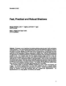
Figure 1: The weighting function applied to a range map of the Sophocle model. From left to right, the input set of samples, the samples colored with their geodesic distance, with their sampling rate and finally with their MLS-based quality.

Also the energy function is formulated in a very intuitive way as the unsigned distance from the surface in terms of the surfel positions and normals. Since we would like to give more relevance to points lying along the surfel normals, the energy function formulation make use of the Mahalanobis distance distM , a distance measure similar to the euclidian one but with elliptical rather than spherical support:


2


2

distM (p, xi ,~ni ) = (p−xi )·~ni +c (p−xi )− (p−xi )·~ni ~ni , where c is a scale factor witch affects the ellipsis shape: in particular when k = 1, the Mahalanobis distance is equivalent to the euclidian distance between the point p and the sample qi , whereas when k = 0 it corresponds to the distance from p to the plane through xi with normal ~ni . The resulting energy function is: ePSS (p,~n) = ePSS (p) = ∑ distM (p, xi ,~ni ) ϑN (p, xi ). i

Finally the implicit surface is determined by the set of points where the energy function e, evaluated along the direction ` of the vector field n, takes its minimum, i.e.: n
o S = p | p ∈ arglocalmin ePSS q, nPSS (p) . q∈`p,nPSS (p)

4. Practical Weighting Scheme As defined so far weighting functions, energy function, and vector field were formulated in the same way for each point in the dataset. A better solution would be to assign to each sample a weight representing the quality of the sample. In the case of sampled data, we may define heuristics which estimate the accuracy of each sample, by taking into account the errors the acquisition pipeline introduces. First of all we must take into account the sampling noise introduced by the scanner: this noise is not uniformly distributed on the whole c The Eurographics Association 2008.

dataset, but can be estimated stronger near the borders of the rangemaps. Some more errors are then introduced during the alignment phase, when the local frames of each rangemap are mapped into a global common frame. At the end of this phase, the set of points from the various range maps are expressed in the same reference frame, and constitutes a single but not uniform distributed point cloud. Indeed each portion of the surface is probably described by more than one rangemap and, almost certainly, each rangemap describes that surface patch at a different sampling density. Therefore using the per-rangemap sampling rate as a measure of the point quality might be restrictive. Conversely, a more reliable measure of the quality for each sample should be the overall sampling rate, since this measure describe very well how points are scattered across the surface of the acquired object. The measure of the quality of each point can be formulated by taking into account all these considerations. The idea underlying our intuition is to weight each sample point both on its position inside the single rangemap and on the position with respect to the whole set of rangemaps. Namely we suggest to enrich each sample point with two distinct attributes, the geodesic distance and the sampling rate, capturing both these characteristics. Once the per-sample geodesic and the sampling qualities are computed, these two measures can be combined with the weighting function of eq. 1, so that the quality assigned to each point p is a function not only of its position but also of the quality of the nearest samples.

4.1. Geodesic blending The geodesic distance is defined here as the length of the minimal path from a point to an open border of the surface. Despite the simplicity of this definition, the geodesic distance computation is not simple, as is not clear what a path

V. Fiorin & P. Cignoni & R. Scopigno / Practical and robust MLS-based integration of scanned data

is on a point cloud. Therefore, the geodesic distance computation can be solved by computing the minimal spanning tree (MST) with multiple sources over the point cloud, where each source corresponds to a sample on the border of the rangemap. Our approach is to see the point cloud as a graph (G, E), where each node in G corresponds to a point in the dataset and E is the set of edges between a point and its k nearest samples, where the weight of an edge is the Euclidean distance between the points corresponding to its vertices. For each point in the graph, the initial geodesic distance attribute is set to ∞. Then the border points are detected and their geodesic distance attribute is set to zero. This sample constitutes the sources of the MST algorithm, and thus they are used to initialize the queue of the visited nodes. This approach requires to solve the problem of detecting the borders of a point cloud. Different solutions have been proposed in the last few years to this problem. The largest projected angle criterion [SFS05] marks a sample as a border one if the maximal angle between the projection of the k nearest samples on the tangent plane at the surface is greater than a threshold angle specified by the user. A more complex approach is proposed in [BSK06] . Here the kε-neighborhood graph is defined and four criteria over this graph are developed aiming to correctly detect the border of a point cloud. The kε-neighborhood graph is a symmetric graph that overcomes the biasing effect that typically affects pointset with variable sampling rate. A robust computation of the overall boundary probability is finally obtained as the average sum of the four criteria. Since this latter approach perform very well in practice (also in presence of noise), we adopted it in our reconstruction tool and used it as preliminary step in the computation of the geodesic distance.

4.2. Data distribution and sampling density A very useful parameter for valuating the goodness of a sample is the sampling density. In many works this parameter is frequently associated with the surface curvature, especially when the reconstruction algorithm needs a greater sampling density in order to be able to accurately reconstruct those area with high curvature; in other works, the sampling density is a measure of the overall quality of a rangemap. We suggest instead to associate to each sample point a value representing the sampling factor at the point. We compute this value regardless of the whole dataset, considered as the union of the points of the various rangemaps, but in relation to the single rangemap during a preprocessing of the dataset. The sampling quality qs we assign to each point is directly proportional to the distance from its kε-neighbors, i.e.: qs =

∑

qi ∈kεNgbh(p)

e

d(qi ,p)2 h2

,

Figure 2: One of the advantages of the MLS operator is the ability to smoothly interpolate between the input samples; however this behavior is not always convenient, especially when we are interest in preserving and correctly reconstructing sharp features.

where h corresponds to the minimum feature size and kε − Ngbh(p) is the kε-neighborhood set for the point p. This way the sampling factor for a point is not a mere measure of the mean sampling, computed for example as the ratio between the dimension of the surface described by a rangemap and the number of samples inside the same rangemap, but an estimate of how much a portion of the surface was visible from the acquisition point: indeed portions of the surface most visible from a certain position will be described by a denser sampling. Furthermore, since the sampling factor is formulated in terms of the distance, the sampling factor assigned to each sample can be compared between points belonging to different rangemaps too. Given this value as measure of the quality of the local sampling, we can combine the sampling factor inside the weighting function of equation 1 used during the application of the projector operator. The weights assigned to points belonging to different rangemaps reflect the sampling quality of the surface for a specific rangemap: points belonging to rangemaps more dense in a given volume portion will have a smaller value for the sampling quality and thus they will influence less the projector operator compared to points belonging to rangemaps less dense in the same volume portion. We point out that specifying the sampling quality through the value k of the neighborhood size guarantees a consistent definition of this quality measure even in undersampled areas: thus samples inside such areas will affect more the projection operator during the reconstruction process than points belonging to denser area. Certainly such a weighting scheme would not seem much reasonable, since it gives more weight to isolated points: however models reconstructed by adopting such a measure in the weighting function did not present the swellings which generally affect surfaces built through the MLS operator. The reasons of a such counter-intuitive behavior are a consequence of MLS operator definition and can be explained with the help of two figures: Figure 2 illustrates a known limitation of the MLS operator, that is its inability to identity sharp features and c The Eurographics Association 2008.

V. Fiorin & P. Cignoni & R. Scopigno / Practical and robust MLS-based integration of scanned data

Figure 3: Reconstruction of a sharp feature from surfaces with different sampling rate. In this case the standard MLS operator not only connects the two surface witch a patch that smoothly interpolate the input samples, but the reconstruction is also asymmetric since the two surfaces have different sampling rate.

to correctly preserve them; conversely, a continuous surface which smoothly interpolates the original sample points is the general behavior of the MLS operator. Figure 3 presents the particular case where two surfaces are described with a very different sampling rate; in this case they are joined by a surface patch which not only interpolates them but is also asymmetric on account of their different sampling rate. Our idea is to increase the influence these samples have on the reconstruction process by increasing their weights. In this way, even though we are not able to completely eliminate the MLS smoothing tendency, however we can see a limitation of such a phenomenon and obtain more faithful reconstructions of the acquired surfaces. 4.3. Locally changing the support of the MLS operator Both measures discussed above are able to capture the quality of each sample in relation to points belonging to the same rangemap. Even thought both the geodesic distance and the sampling rate are expressed in such a way that their values are meaningful when compared between different rangemaps, a global measure is still needed. We suggest to introduce a new global quality measure that can be exploited to face with misalignment errors: being able to correctly detect areas where rangemaps are not well aligned, we can guarantee the reconstruction of a single coherent surface. The necessity to introduce such a new measure results from the observation that the reconstruction algorithm lacks of the necessary information to detect if two slightly overlapped sheets in the same volume portion actually describe the same surface; besides, neither the sampling rate nor the geodesic distance are useful to detect such situations. Our idea is to take advantage of the smoothing ability of the MLS operator and to use it to extract a height map where to each sample point is assigned the magnitude of the shift the MLS operator impose on it. In other words, given a neighborhood size n, we apply the MLS operator to a random subset of the whole point cloud, and for each of them we record how much each point has been shifted when projected onto the surface. c The Eurographics Association 2008.

Since misalignment errors are not local but they spread over large portion of the dataset, adopting a monte-carlo approach does not preclude the effectiveness of the measure. In order to guarantee that each point come with its own value, we developed two strategies for spreading the sampled values across the whole dataset: both these strategies take advantages of the previous consideration, namely the fact that the misalignment error is by definition a error that involves whole areas rather than isolated sample points. The first strategy is as follows: for each point in the dataset, we look for its neighbors and assign to each point the maximum value over its neighboring samples. We repeat this process for a number k of iteration chosen by the user. In this manner the local maxima spread across small surface patches, in a way that mimic the nature of misalignment errors. In order to guarantee that a meaningful value is assigned to each sample point, a clustering step finally completes the computation. During this phase we traverse the octree used to index the whole point cloud, and analyze the samples contained in each of its leaves: if a sample has not been reached during the previous phase, than we assign it a value computed as average of the values of the other samples contained in the same octree leaf. The combination of the two previous strategies allow us to assume that a valid quality value is assigned to each sample. Since we can think of this quality as a measure of the local misalignment error, we use this property for locally changing the MLS support during the reconstruction phase: therefore, where this measure reaches greater values, the samples are distributed on different surface sheets, and thus we need a broader support in order to define a single surface; on the other hand, where this measure reaches lower values, the rangemaps are well-aligned and a small number of points is needed to define a single surface path.

5. Surface Extraction The combined use of both of sampling and geodesic qualities in the projector operator allows us to obtain an implicit surface that continuously and smoothly approximates the pointset. However such a implicit description isn’t very practical to work with, and so an explicit description such as a simplicial mesh is generally needed. As suggested by many authors as well, a simplicial mesh can be efficiently generated by combining a polygonalization algorithm with a distance field regularly sampled at discrete intervals in space. A signed distance function can be obtained from the results generated by the projection procedure. As said before, what we obtain when we apply the projection operator to a point p is the projection along the direction defined by the vector field at p of that point on the nearest implicit surface: in other words, the application of the projection operator to a point p gives back a point-direction pair (p? ,~n? ) that we can

V. Fiorin & P. Cignoni & R. Scopigno / Practical and robust MLS-based integration of scanned data

Figure 4: The weighting function values on the synthetic model: plane disposition (left); samples colored by their geodesic distance (center) and by sampling rate (right).

Figure 5: Reconstruction of the synthetic models without and with the use of the weighting function on the left and on the right respectively.

interpreter as the projection of the point p on the surface and the direction it has been projected along respectively. Furthermore, since the projection operator is recursively defined until a stationary point is obtained, the direction ~n? ) can be considered a good approximation of the surface normal because it has been computed when convergence is reached. The pair (p? ,~n? ) allows us to define the plane P, passing through p? and having direction ~n? , which comes out to be the best local approximation of the portion of the surface nearest to the original point p. We use this plane to estimate the distance between the point p and the implicit surface: thus the distance d(p, P) between the point p and the plane P corresponds to the magnitude of the shift the projection operator has imposed on the point p. Through this signed distance function we are now able to define the scalar field that, together with a polygonalization algorithm, allows us to extract a polygonal model from the implicit representation. The approach we follow is simple but at the same time robust and straightforward: we sample the signed distance function at the corners of the leaves of an octree used to index the point cloud. Since the leaves of the octree cover only the portion of the volume where sample points are distributed, limiting the sampling only at these leaves reduces the number of samplings needed to build a polygonal surface. At the moment we generate the polygonal description of the surface through the Marching Cubes [LC87] and the Extended Marching Cubes [KBSS01] algorithms. 6. Results We integrated the weighting measures presented in the previous section with the reconstruction tool described in [FCS07]. We initially analyze the result obtained by reconstructing a synthetic model: this will provide a deeper com-

Figure 6: Here two planes with the same sampling rate are reported, same spatial position as the previous example.

Figure 7: Here two planes with the same sampling rate are reported: we maintain for each plane the same spatial position as the previous example. On the center and on the right the samples are colored with their value of the geodesic and sampling functions respectively.

prehension of the meaning of the weights and thus will give us the opportunity to better explain how the MLS projection operator and the reconstruction algorithm are influenced by these weights. Then we will present results obtained during the reconstruction of a gargoyle model, a real dataset acquired with a laser-triangulation scanner. The synthetic example is constituted by two planes, both perpendicular to the z axis but slightly shifted, in order to simulate a misalignment error, and partially overlapped (see Figure 4). The two planes have different density: the plane on the right is one third denser that the plane on the left. In the center and on the right of Figure 4 the planes are colored with the per-sample value of the geodesic and density function respectively. In order to show how these functions impact the MLS projector operator, we have reported the models obtained with and without the use of these values in Figure 5, where we have the result of the standard MLS operator on the left (three different steps are easily identifiable in the reconstructed surface); conversely, those steps disappear in the surface on the right, which has been reconstructed by using the sampling and geodesic weights (where different heights of the samples are gradually merged). Moreover the surface extracted is closer to the plane with greater sampling rate. A similar experiment has been run on two planes, with the same spatial configuration of the previous example, but having the same sampling resolution (Figure 6) The surface obtained by using the original definition of the MLS projector operator presents now two pronounced steps next to the area where the two planes overlap (see Figure 7, left), while the surface obtained by adopting our weighting scheme is more smooth; moreover, since the two planes have same resolution and thus their samples have same values for both geodesic c The Eurographics Association 2008.

V. Fiorin & P. Cignoni & R. Scopigno / Practical and robust MLS-based integration of scanned data

Figure 9: The reconstructed gargoyle: standard MLS is on the left, weighted one is on the right. Figure 8: The gargoyle dataset: input point cloud and geodesic distance, sampling rate and MLS quality mapped on a color ramp.

and sampling function, the two surfaces are bridged by a continuous patch, which is exactly at the same distance by both the planes and that smoothly interpolate the drop. The third experiments was run on the Gargoyle pointset (around 800K points sampled by eight range maps acquired with a Konica Minolta VI910 scanner), which due to the material characteristics is quite noisy sampling (see Figure 8 left). Moreover, a glaring misalignment error is present on the gargoyle’s left wing. For these reason we believed this dataset was a good assessment test-bed. We reconstructed the gargoyle’s model first by adopting the standard MLS projector operator, and then by constraining its behavior with the quality measures. The gargoyle’s samples are colored with their geodesic, sampling and MLS quality measures in Figure 8. As expected, where the surface was regularly sampled, the two reconstructed models do not present visible differences (see Figure 9). On the other hand, visible differences were present next to the misalignment error on the left wing or, in general, where the surface has a sudden change in curvature: zoom-in views are presented in Figure 9, without the use of the weights (left) and with the use of the weights (right). 7. Conclusions and future work We have presented three practical quality measures that can be directly computed on a pointset without the need of additional topological information. These measure are based on the geodesic distance and on the sampling rate and are able to capture the degree of importance of each sample. The c The Eurographics Association 2008.

Range map R00 R01 R02 R03 R04 R05 R06 R07

Samples 115K 92K 95K 89K 108K 111K 74K 101K

Graph 15.67s 10.75s 16.47s 15.51s 14.13s 16.05s 15.91s 20.19s

Geodesic 24.45s 18.33s 25.63s 24.56s 22.63s 24.39s 24.08s 29.56s

Sampling 1.67s 1.66s 1.70s 1.67s 1.88s 1.67s 1.67s 1.67s

Table 1: Times needed to compute our weights on the rangemaps for the gargoyle model. We do not included the time for the MLS weight because, unlike the geodesic and the sampling quality which are a per-rangemap measure, this is a global measure computed on the whole point cloud. For this model, consisting of 785K samples, computing the MLS quality took 217.84 seconds.

values these measures take over the pointset are used by a new weighting function to influence the behavior of the MLS projection operator adopted by our reconstruction algorithm. Differences between models reconstructed with and without the use of these weights have been discussed in the result section. Visual differences underline the effectiveness of the quality measures introduced, since surfaces defined through the new weighting function are turned out to be more robust in front of sudden changes in the sampling rate as well as in front of misalignment error between the input range maps. References [AA03a] A DAMSON A., A LEXA M.: Approximating and intersecting surfaces from points. In SGP ’03: Proceedings of the 2003 Eurographics/ACM SIGGRAPH symposium on Geometry

V. Fiorin & P. Cignoni & R. Scopigno / Practical and robust MLS-based integration of scanned data processing (Aire-la-Ville, Switzerland, Switzerland, 2003), Eurographics Association, pp. 230–239. [AA03b] A DAMSON A., A LEXA M.: Ray tracing point set surfaces. In SMI ’03: Proceedings of the Shape Modeling International 2003 (Washington, DC, USA, 2003), IEEE Computer Society, p. 272. [AB98] A MENTA N., B ERN M. W.: Surface reconstruction by voronoi filtering. In Symposium on Computational Geometry (1998), pp. 39–48. [ABCO∗ 01] A LEXA M., B EHR J., C OHEN -O R D., F LEISHMAN S., L EVIN D., S ILVA C. T.: Point set surfaces. In VIS ’01: Proceedings of the conference on Visualization ’01 (Washington, DC, USA, 2001), IEEE Computer Society, pp. 21–28. [AK04a] A MENTA N., K IL Y. J.: Defining point-set surfaces. In SIGGRAPH ’04: ACM SIGGRAPH 2004 Papers (New York, NY, USA, 2004), ACM Press, pp. 264–270. [AK04b] A MENTA N., K IL Y. J.: The domain of a point set surfaces. Eurographics Symposium on Point-based Graphics 1, 1 (June 2004), 139–147. [BBX95] BAJAJ C. L., B ERNARDINI F., X U G.: Automatic reconstruction of surfaces and scalar fields from 3D scans. Computer Graphics 29, Annual Conference Series (1995), 109–118. [BMR∗ 99] B ERNARDINI F., M ITTLEMAN J., RUSHMEIER H., S ILVA C., TAUBIN G.: The ball-pivoting algorithm for surface reconstruction. IEEE Transactions on Visualization and Computer Graphics 5, 4 (Oct.-Dec. 1999), 349–359. [BSK06] B ENDELS G. H., S CHNABEL R., K LEIN R.: Detecting holes in point set surfaces. Journal of WSCG 14 (February 2006). [CBC∗ 01] C ARR J. C., B EATSON R. K., C HERRIE J. B., M ITCHELL T. J., F RIGHT W. R., M C C ALLUM B. C., E VANS T. R.: Reconstruction and representation of 3D objects with radial basis functions. In SIGGRAPH 2001, Computer Graphics Proceedings (2001), Annual Conference Series, ACM Press / ACM SIGGRAPH, pp. 67–76. [CBM∗ 03] C ARR J. C., B EATSON R. K., M C C ALLUM B. C., F RIGHT W. R., M C L ENNAN T. J., M ITCHELL T. J.: Smooth surface reconstruction from noisy range data. In GRAPHITE ’03: Proceedings of the 1st international conference on Computer graphics and interactive techniques in Australasia and South East Asia (New York, NY, USA, 2003), ACM Press, pp. 119–ff. [CL96] C URLESS B., L EVOY M.: A volumetric method for building complex models from range images. In Comp. Graph. Proc., Annual Conf. Series (SIGGRAPH 96) (1996), ACM Press, pp. 303–312. [DBL05] :. Third Eurographics Symposium on Geometry Processing, Vienna, Austria, July 4-6, 2005 (2005). [DS05] D EY T. K., S UN J.: . an adaptive mls surface for reconstruction with guarantees. In Symposium on Geometry Processing [DBL05], pp. 43–52. [EM94] E DELSBRUNNER H., M ÜCKE E. P.: Three-Dimensional alpha shapes. ACM Transactions on Graphics 13, 1 (Jan. 1994), 43–72. ISSN 0730-0301. [FCOS05] F LEISHMAN S., C OHEN -O R D., S ILVA C. T.: Robust moving least-squares fitting with sharp features. ACM Trans. Graph. 24, 3 (2005), 544–552.

[FCS07] F IORIN V., C IGNONI P., S COPIGNO R.: Out-of-core mls reconstruction. In Proc. of he Ninth IASTED International Conference on Computer Graphics and Imaging (CGIM) (2007), pp. 27–34. [HDD∗ 92] H OPPE H., D E ROSE T., D UCHAMP T., M C D ONALD J., S TUETZLE W.: Surface reconstruction from unorganized points. Computer Graphics 26, 2 (1992), 71–78. [HWC∗ 05] H O C.-C., W U F.-C., C HEN B.-Y., C HUANG Y.Y., O UHYOUNG M.: Cubical marching squares: Adaptive feature preserving surface extraction from volume data. Computer Graphics Forum 24, 3 (August 2005), 537–545. Special issue: Proceedings of EUROGRAPHICS 2005. [JLSW02] J U T., L OSASSO F., S CHAEFER S., WARREN J.: Dual contouring of hermite data. In Siggraph 2002, Computer Graphics Proceedings (2002), ACM Press / ACM SIGGRAPH / Addison Wesley Longman, pp. 339–346. [Joe]

J OE S. S.: Dual contouring: The secret sauce.

[KBSS01] KOBBELT L., B OTSCH M., S CHWANECKE U., S EI DEL H.: Feature-sensitive surface extraction from volume data. In SIGGRAPH 2001, Computer Graphics Proceedings (2001), Fiume E., (Ed.), ACM Press / ACM SIGGRAPH, pp. 57–66. [Kol05] KOLLURI R.: Provably good moving least squares. In Proceedings of ACM-SIAM Symposium on Discrete Algorithms (Aug. 2005), pp. 1008–1018. [LC87] L ORENSEN W. E., C LINE H. E.: Marching cubes: A high resolution 3D surface construction algorithm. In ACM Computer Graphics (SIGGRAPH 87 Proceedings) (1987), vol. 21, pp. 163– 170. [Lev98] L EVIN D.: The approximation power of moving leastsquares. Mathematics of Computation 67, 224 (1998), 1517– 1531. [LLVT03] L EWINER T., L OPES H., V IEIRA A. W., TAVARES G.: Efficient implementation of marching cubes’ cases with topological guarantees. Int. Journal of Graphics Tools 8, 2 (2003), 1–15. [OBA∗ 03] O HTAKE Y., B ELYAEV A., A LEXA M., T URK G., S EIDEL H.-P.: Multi-level partition of unity implicits. ACM Transactions on Graphics 22, 3 (July 2003), 463–470. [RJT∗ 05] R EUTER P., J OYOT P., T RUNZLER J., B OUBEKEUR T., S CHLICK C.: Surface reconstruction with enriched reproducing kernel particle approximation. In Proceedings of the IEEE/Eurographics Symposium on Point-Based Graphics (2005), Eurographics/IEEE Computer Society, pp. 79–87. [SFS05] S CHEIDEGGER C. E., F LEISHMAN S., S ILVA C. T.: Triangulating point set surfaces with bounded error. In Symposium on Geometry Processing [DBL05], pp. 63–72. [SOS04] S HEN C., O’B RIEN J. F., S HEWCHUK J. R.: Interpolating and approximating implicit surfaces from polygon soup. ACM Trans. Graph. 23, 3 (2004), 896–904. [SW04] S CHAEFER S., WARREN J.: Dual marching cubes: Primal contouring of dual grids. In PG ’04: Proceedings of the Computer Graphics and Applications, 12th Pacific Conference on (PG’04) (Washington, DC, USA, 2004), IEEE Computer Society, pp. 70–76. [TL94] T URK G., L EVOY M.: Zippered polygon meshes from range images. ACM Computer Graphics 28, 3 (1994), 311–318. c The Eurographics Association 2008.