Q IWA Publishing 2010 Water Science & Technology—WST | 61.6 | 2010
1561
Practical applications of quantitative microbial risk assessment (QMRA) for water safety plans P. W. M. H. Smeets, L. C. Rietveld, J. C. van Dijk and G. J. Medema
ABSTRACT The absence of indicator organisms in drinking water does not provide sufficient guarantee for microbial safety. Therefore the water utilities are implementing water safety plans (WSP) to safeguard drinking water quality. Quantitative microbial risk assessment (QMRA) can be used to provide objective quantitative input for the WSP. This study presents several applications of
P. W. M. H. Smeets G. J. Medema KWR Watercycle Research Institute, PO Box 1072, 3430 BB Nieuwegein, The Netherlands E-mail:
[email protected]
treatment modelling in QMRA to answer the risk managers questions raised in the WSP. QMRA can estimate how safe the water is, how much the safety varies and how certain the estimate of safety is. This can be used in the WSP system assessment to determine whether treatment is meeting health-based targets with the required level of certainty. Quantitative data analysis showed that short events of only 8 hours per year can dominate the yearly average health risk for the consumer. QMRA also helps the design of physical and microbial monitoring.
P. W. M. H. Smeets L. C. Rietveld J. C. van Dijk Faculty of Civil Engineering, Delft University of Technology, PO Box 5048, 2600 GA Delft, The Netherlands
The study showed that the required monitoring frequency increases with increasing treatment efficacy. Daily monitoring can be sufficient to verify a treatment process achieving 2 log reduction of pathogens, but a process achieving 4 log reduction needs to be monitored every 15 minutes. Similarly, QMRA helps to prepare adequate corrective actions by determining the acceptable ‘down time’ of a process. For example, for a process achieving 2.5 log reduction a down time of maximum 6 hours per year is acceptable. These applications illustrate how QMRA can contribute to efficient and effective management of microbial drinking water safety. Key words
| QMRA, water safety plans
INTRODUCTION The goal of the water safety plan (WSP) is to manage water
risks. A ‘tier one’ level of risk assessment is often applied,
supply such that health-based targets are met (Davison et al.
using log credits (indicating the level of reduction of
2006). To determine if the health-based targets are met, the
pathogens in log units) and CT tables (where CT refers to
risk of infection from the supplied water needs to be
the product of the disinfectant concentration and the
assessed. Qualitative and semi-quantitative estimates of risk
contact time) to quantify treatment efficacy (Davison et al.
have been applied in WSP, such as the risk matrix (Davison
2006). Log credits could be effective at a screening level
et al. 2006). The risk matrix relies on the previous
quantitative microbial risk assessment (QMRA) to prioritize
experiences of those involved in the WSP development.
between different sites and to identify sites that may not
The risk matrix requires detailed quantitative judgement on
achieve the health-based targets (Medema et al. 2006).
the effect of a risk such as ‘compliance impact (minor)’ or
However, log credits do not account for site specific
‘public health impact (catastrophic)’. This method leads to a
conditions and variations of treatment efficacy in time and
subjective judgement of risk that is suitable to identify ‘clear’
the uncertainty involved (Teunis et al. 2009). In QMRA the
doi: 10.2166/wst.2010.839
1562
P. W. M. H. Smeets et al. | Practical applications of QMRA for water safety plans
Water Science & Technology—WST | 61.6 | 2010
risk of infection from drinking water from a treatment
treatment efficacy, pf is the treatment efficacy during failure
system is assessed by identifying the pathogen sources,
and pf is the proportion of time that failure occurs.
monitoring pathogens in source water, describing treatment performance, contamination during distribution and consumption and applying dose-response relations (Haas et al. 1999; Smeets et al. 2008). Acceptable risk levels referred to in guidelines and legislation are very low, in the order of 1 infection per 10,000 people per year (Anonymous 2001; WHO 2004), so effective treatment is crucial for safe drinking water production. QMRA can quantify whether adequate operation and sufficient monitoring was per-
aacc pn $ pf pf
ð1Þ
The probability of detecting a failure event was calculated with Equation (2). Assuming that monitoring indicated either “non-failure” or “failure” of the process, the chance of detecting a failure event pd could be determined from the chance of failure pf and the number of samples N: pd ¼ 1 2 ð1 2 pf ÞN
ð2Þ
formed to verify that the water was safe. This paper illustrates how QMRA can be used in the WSP to design microbial and non-microbial monitoring, set critical limits
The mean treatment efficacy including failures pm was calculated as:
and prepare corrective actions based on quantitative information to achieve treatment goals.
pm ¼ ð1 2 pf Þpn þ pf pf
ð3Þ
The average yearly treatment efficacy including corrective actions was calculated with Equation (4) which is
METHODS Operational treatment data was collected in the MicroRisk project (Smeets 2008). This data was used in to illustrate
similar to Equation (3) but included three situations: nominal treatment, failure and corrective treatment.
pm ¼ ð1 2 pf 2 pc Þpn þ pf pf þ pc pc
ð4Þ
the preparation of corrective actions in case of chlorine dosage failure. UK statutory Cryptosporidium monitoring
where pc was the proportion of time that corrective
data was collected through the UK statutory Cryptospo-
treatment was performed and pc was the treatment efficacy
ridium monitoring program. All surface water treatment
during corrective treatment.
systems perform daily continuous monitoring for at least 23 hours, filtering 40 L/h of their produced drinking water. This results in approximately 1,000 L samples that are analysed for Cryptosporidium. The data is described in more detail in (Smeets et al. 2007). Data was presented in
RESULTS Design of microbial monitoring
a complementary cumulative frequency distribution by
Microbial monitoring before and after a treatment process,
sorting the reported concentrations, including negative
is the most direct way to assess treatment efficacy.
samples, and attributing an equal proportion of time to
Furthermore microbial monitoring of drinking water could
each sample. By cumulating the proportions, a CCDF was
also provide a direct assessment of drinking water safety.
plotted so that each point indicates the proportion of time
The microbial monitoring needs to provide a reliable
that a concentration was exceeded.
estimate of the arithmetic mean concentration for both
The effect of short events of poor treatment on the
these applications. When organisms in water are over
yearly average treatment efficacy was calculated as follows.
dispersed, high concentrations that rarely occur can still
A loss of treatment efficacy due to a special event, e.g. a
dominate the mean concentration. Monitoring will provide
clogged dosing pump, was referred to as a failure.
a range of microorganism concentrations, from which the
The acceptable risk criteria for failures were expressed in
mean concentration is calculated. A question from the risk
the form of Equation (1) where aacc is the acceptable
manager could be: Have I taken enough samples to
contribution of failures to average risk, pn is the nominal
determine the mean microorganism concentration in the
P. W. M. H. Smeets et al. | Practical applications of QMRA for water safety plans
1563
Water Science & Technology—WST | 61.6 | 2010
water? To answer this question, the risk manager needs to
A complicating factor is the occurrence of ‘special
determine whether the “dominant concentrations” have
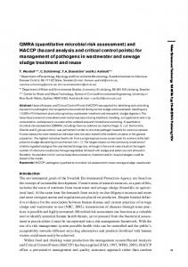
events’. Figure 1a shows the concentrations due to normal
been determined by monitoring. The answer to this question
variations, so high concentrations can be considered
is illustrated through Figures 1a, b and 2. The markers show
‘normal events’. Figure 1b shows a ‘special event’ where
the observed Cryptosporidium concentrations in drinking
very high concentrations occurred e.g. due to human error
water at three treatment sites in the UK from 2000 to
or equipment failure causing a curve break. In Figure 1b the
2002. The contribution of each monitored concentration to
dashed line touches the markers at the highest monitored
the mean was determined as the product of the concen-
concentration. The concentration during the special event
tration and the proportion of the drinking water exceeding
therefore dominated the average concentration and thus the
that concentration. A low concentration of 0.01 organism/L
yearly average risk at this site. These special events were
exceeded 100% of the time resulted in the same contri-
observed in 10% of the datasets from 216 treatment sites in
bution to the mean concentration as a high concentration of
the UK. At the example site in Figure 1b, other monitoring
1 organism/L exceeded 1% of the time. The dashed line
efforts, apart from microbial monitoring, would be required
shows combinations of proportion and concentration that
to verify that these special events did not occur even for a
contributed equally to the mean concentration. The
few hours per year (a proportion of 1023 translates into
arithmetic mean concentration at the site in Figure 1a was
eight hours per year). Methods for event monitoring will be
0.002 oocysts/L. The observed concentrations between
discussed later.
23
2 £ 10
and 10
22
oocysts/L dominated this mean
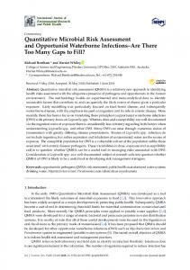
A second complicating factor is the detection limit
concentration. This is where the dashed line touches the
or sample volume. At treatment sites with lower concen-
markers of the observed concentrations. Based on this data,
trations of Cryptosporidium in the treated water, the
the average concentration was accurately determined, since
observed concentrations looked like Figure 2 which was
higher and lower concentrations would not contribute
typical for 60% of the monitored UK sites.
significantly to the mean concentration. This typical shape
The arithmetic mean concentration was 6 £ 1025
was found for 30% of the 216 treatment sites for which data
oocysts/L based on the monitoring results. This mean
had been collected. Dominant concentrations generally
concentration was dominated by the lowest observed
occurred in less then 1%–5% of the samples in raw water,
concentration (at the detection limit) of 7 £ 1024 oocysts/L
during treatment and in drinking water. So in order to generate
exceeded 7% of the time. However, an intuitive inter-
a usable estimate of the risk, over 20 to 100 microbial samples
polation to lower concentrations would exceed the
at any point in the system would typically be required.
dashed line, thus dominating the mean concentration and
Figure 1
|
Monitored Cryptosporidium in drinking water (markers) including normal events (a) and special events (b). The dashed line indicates combinations of proportion and concentration resulting in the same average concentration.
P. W. M. H. Smeets et al. | Practical applications of QMRA for water safety plans
1564
Water Science & Technology—WST | 61.6 | 2010
could be quantified in more detail this could be incorporated in the calculations. First the acceptable level of increase of risk due to failure aacc in Equation (1) needs to be chosen. The risk due to the event will add to the nominal risk. Risks due to special events might result in a higher average risk than the nominal risk, which would not be considered acceptable. In this example the risk from failures is considered acceptable when on average it equals the nominal risk, so aacc equals 1. A more strict condition could be set by choosing a lower value for aacc. Complete failure of the treatment process during an event was assumed in this example, so treatment efficacy during failure pf equalled 1. In that case the acceptable proportion of time that failure occurs pf equalled Figure 2
|
Monitored Cryptosporidium in drinking water (markers). The dashed line indicates combinations of proportion and concentration resulting in the same average concentration.
nominal reduction pn. The probability of detecting a failure
therefore the average risk. Larger volumes taken at a lower
monitoring indicated either “non-failure” or “failure” of
event was calculated with Equation (2) assuming that
frequency could be used to determine the dominating
the process. By choosing the probability of detection pd at
concentration. Stochastic modelling of the treatment as
the desired confidence level (e.g. 90%, 95%, 99%) the
performed in QMRA could provide an estimate of these low
required number of measurements N could be calculated.
concentrations (Smeets et al. 2008), based on raw water
The safety of the system is verified when no failures are
concentrations and removal by treatment.
detected with N measurements over the assessed period. Table 1 shows the required number of measurements in relation to the nominal log reduction to verify at the 95%
Design of process monitoring When the treatment assessment in the WSP indicates that the system is capable of producing safe water, the system needs to be monitored to verify that treatment targets were met. Therefore one of the monitoring goals is to verify that no special events have occurred that could have a
confidence level that failure events did not significantly increase the risk. The monitoring frequency for the assessment of a one year period was also calculated. Approximately 30% less measurements are required for a 90% confidence level, respectively 50% more measurements are required for a 99% confidence level.
significant impact on the assessed risk (Figure 1b). Since this often requires very frequent monitoring, microbial
Table 1
monitoring is generally not feasible. However, other parameters that may be monitored on-line can be used to verify the system was working as expected. Equipment monitoring such as dosing pump flow can also be used to verify that the system was operational, or to detect moments of failure. Deviation of any of these parameters could lead to reduced treatment efficacy, which may be hard to quantify. A conservative approach is to assume complete failure in case of a deviance. The following examples assume that monitoring either indicates compliance or failure (no pathogen reduction), however if efficacy during failure
|
Number of required monitoring records to verify at the 95% confidence level that failure events do not significantly add to the risk when compared to nominal reduction
Nominal log reduction
#/year
Monitoring interval
0.05
1
1 year
1
30
1 week
2
300
1 day
3
3,000
3 hours
4
30,000
15 min
5
300,000
2 min
6
3,000,000
10 sec
7
30,000,000
1 sec
1565
P. W. M. H. Smeets et al. | Practical applications of QMRA for water safety plans
Water Science & Technology—WST | 61.6 | 2010
Table 1 shows that with daily sampling, no more than 2 log reduction can be verified. Above that, more frequent monitoring is required, leading to on-line monitoring. Some treatment plants claim 7 log inactivation of viruses with a disinfection system, so at a 100,000 m3/d plant every 3 litres must be monitored to be 95% confident that all water was sufficiently treated. If the criteria are set stricter, for example setting aacc to 10%, ten times as many samples are required. A multiple barrier system is easier to monitor. When 6 log inactivation is achieved through 1 barrier (treatment process) 3 million measurements per year are required. The continuous measurement of UV radiation intensity is an example of such intensive monitoring to verifying absence of failure of the highly effective UV disinfection process. When three barriers of 2 logs are placed in series, only 300 measurements per year are required for each process, resulting in 900 measurements in total. So daily monitoring of each process step is then sufficient. This approach assumes that treatment process failures are independent and that
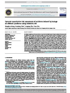
Figure 3
|
Simulated example of critical limits, operational limits, setpoints and monitoring of a chlorine disinfection process.
to operational variation. Chlorine dosing was controlled by an automatic control loop in this example. The chlorine residual was measured and the dosing rate was adjusted if the measured concentration deviated from the setpoint. As a
failure of the first step does not automatically coincide with
result, the chlorine residual level would typically vary
failure of the second step. Risk managers can minimise the
between the operational limits if the system was working
risk of such consecutive failures in their design of the process
within specification, as indicated in Figure 3.
for example by separating power supplies and placing
At hour 20 the chlorine dosing pump got clogged,
physical barriers between equipment so that physical
resulting in a chlorine level below the lower operational
hazards (e.g. flooding or fire) would not affect both processes.
limit. This triggered an alarm and the operator was able to clean the pump and restore normal operation. This event did not affect the average treatment performance in a way
Setting critical limits
that the health-based target would not be met, since the
A treatment system can be designed to provide exactly the
critical limit was not exceeded. At hour 80 the chlorine
right level of treatment to meet the health-based targets.
dosing pump failed again, however this time the operator
However, in practice the risk manager needs to account for
was not in time to restore the system before the critical limit
variations and inaccuracies in order to run a practical and
was exceeded. The short period of time that disinfection was
stable process. The simulated example in Figure 3 is used to
ineffective reduced the average treatment efficacy since the
illustrate how QMRA can be used to set critical limits and
critical limit was exceeded. Therefore the operator needed
setpoints. The health-based treatment target for the disinfec-
to take corrective actions, such as starting emergency
tion process simulated in Figure 3 was 3 log inactivation of
chlorination of the distributed water, in order to achieve
viruses. In this example the temperature and flow conditions
the health-based target over the total period.
were constant for the whole period. The required chlorine
This example illustrated that setting critical limits was
residual of 1.7 mg/l for 3 log inactivation was determined by
not merely determining the lowest chlorine dose to meet the
disinfection modelling. So if the process was constantly run at
target, but also included setting operational setpoints and
exactly this concentration, the yearly health-based target
operational limits. Quantifying limits and setpoints is
would be met. This level is therefore considered the critical
related to many site specific issues such as the treatment
limit. However, in practice the chlorine dose would vary due
target, the normal variability of the process, the probability
1566
P. W. M. H. Smeets et al. | Practical applications of QMRA for water safety plans
Water Science & Technology—WST | 61.6 | 2010
of events, the response time of the operator and the effect of
All treatment steps were considered to be independent
corrective actions. Simply applying a higher setpoint for
in this study. In practice some interaction between treat-
chlorine dose can have adverse effects in other objectives
ment steps can be expected. Positive interaction occurs
(cost, Disinfectant By-Product (DBP) formation, mainte-
when failure at one step leads to failure of a consecutive
nance/operation) and therefore is not an option. QMRA
step(s). For example, failure of pre-oxidation leads directly
can provide decision support for choosing setpoints and
to less inactivation, but also increases oxidant demand at a
limits when some realistic assumptions are made. The mean
later disinfection step, thereby reducing its efficacy. Nega-
treatment efficacy over a period was calculated with
tive interaction can occur when failure at an early step leads
Equation (3). The proportion of time that the system fails
to increased performance of a consecutive step, e.g. poor
pf and treatment efficacy during failure pf can be roughly
sedimentation increases particle load to the filters which
quantified by means of the risk matrix in the WSP. In the
then work more effectively. Although these mechanisms
example it was assumed that operator response could take
have been observed, current knowledge is insufficient to
up to 8 hours to restore the system to normal operation, an
create a deterministic model that describes these relations.
event could occur once a year and disinfection would fail completely during an event. Given these assumptions, pf was 8/(365 £ 24), pf equalled 1 and pm equalled 0.001
Preparing corrective actions
(3 log reduction). Using Equation (3) the nominal treatment
Even at a well managed system failures can occur that
efficacy pn to achieve pm was 0.000085 (4.1 log reduction).
compromise drinking water safety. Such events could be
Disinfection modelling showed that a chlorine residual of
detected by monitoring. A temporal decrease of drinking
2 mg/l was required to achieve 4.1 log reduction, therefore
water quality could have a significant effect on the yearly
the lower operational limit was set to 2 mg/l. Due to normal
average risk. When critical limits are exceeded, corrective
variation in the process, observed from hour 25 to 75 in
actions need to bring back water quality to an acceptable
Figure 3, a setpoint of 2.3 mg/l was needed to maintain this
level to comply with the yearly risk of infection. This is
limit. This example illustrated the basic approach to setting
illustrated with the example of chlorine inactivation of
limits and setpoints. The method could be adapted to
viruses in Figure 4. The target inactivation by this system
include other variables such as temperature and flow
was 2.5 logs, which was generally achieved through process
variations and partial treatment failure.
control. The risk manager would need to prepare a plan for
One of the objectives of the multiple barrier system is to
corrective actions if failure occurred. Shutting down
balance out peaks or failure at one point by adequate
treatment completely in case of failure was not an option
treatment at another point. Total pathogen reduction at a
since this would disrupt the other processes and the
surface water treatment site is often many orders of
distribution system would loose pressure thus risking
magnitude due to a large number of treatment steps. The total treatment can be optimized such that the combination of reduction by individual treatment steps combined provides exactly the required reduction to meet the health-based targets. This could be extended to an on-line control tool for pathogen reduction to respond to changes in process conditions. The disinfection model could be used in an algorithm programmed into an automatic operation system to constantly adjust the critical limits, operational limits and setpoint for chlorine dosing to maintain the target level of inactivation. The treatment would thus be controlled by the combined effect of process conditions rather than control of individual parameters.
Figure 4
|
Virus inactivation by chlorine based on chlorine residual monitoring (black line), the level of inactivation during corrective actions (grey line) and the yearly average inactivation that could be achieved by corrective actions in relation to the time required to start corrective actions (dashed line).
1567
P. W. M. H. Smeets et al. | Practical applications of QMRA for water safety plans
Water Science & Technology—WST | 61.6 | 2010
ingress of contaminated water into the distribution system.
QMRA the system assessment in the WSP relies on risk
An emergency UV disinfection unit which could achieve
manager experience and log-credits from industry standards
4.5 log inactivation of viruses was considered as a corrective
to quantify drinking water safety. QMRA does not only tell
measure. The first question for the risk manager was how
us how safe the water is, but also how much the safety varies
quickly the emergency equipment needed to be in place. Or,
and how certain we are that we are meeting health-based
stated differently: how long could this failure be allowed to
targets. The QMRA methods presented in this study can be
continue without compromising the treatment target?
used to quantify and reduce uncertainties by using site
QMRA could be used to answer this question. Figure 4
specific full-scale information. QMRA can be used in the
shows the calculated virus inactivation based on monitored
system assessment and provides decision support on other
chlorine residual concentration. During normal operation
issues of the WSP. This study provided examples of QMRA
from 27 April to 19 May, generally 2.5 to 3 log inactivation
applications to design physical and microbial monitoring, to
was achieved (black line), resulting in a running average
set critical limits, and to prepare corrective actions. Thus
inactivation that complies with the target of 2.5 log
QMRA can contribute to efficient and effective manage-
inactivation. On 20 May the chlorine dosing failed
ment of microbial drinking water safety.
completely (as an example), resulting in no disinfection. The grey line shows the level of inactivation that could be achieved with the emergency equipment. The average yearly
ACKNOWLEDGEMENTS
treatment efficacy was calculated for different response times with Equation (4). In this example pm and pn were
The research was funded by the MicroRisk project and the
0.0032 (2.5 log reduction), pc was 0.000032 (4.5 log) pn was
joint research program of the Dutch water companies.
139/365 (days until 20 May), pc was 1 2 pn 2 pf and pf
The MicroRisk (www.microrisk.com) project is co-funded
varied between 0 hours and 17 days.
by the European Commission under contract number
The dashed line in Figure 4 shows the achievable yearly
EVK1-CT-2002-00123.
average inactivation in relation to the time the corrective action is started. It was clear from Figure 4 that the achievable yearly average quickly decreased in time. In this example, corrective measures needed to be taken within six and a half hours in order to comply with the yearly target of 2.5 log reduction. Risk managers can use similar calculations for decision support on emergency measures and emergency procedures in relation to the health-based treatment target, the critical limits of the treatment process and the achievable corrective action.
CONCLUSIONS Water utilities have started to use water safety plans (WSP) to assess and improve the safety of the produced drinking water. Resources for assessments and improvements are limited and therefore need to be used effectively and efficiently to provide the most benefit for health. Quantitative microbial risk assessment can be used to quantify several questions that are raised in the WSP. Without
REFERENCES Anonymous 2001 Adaptation of Dutch drinking water legislation. Besluit van 9 januari 2001 tot wijziging van het waterleidingbesluit in verband met de richtlijn betreffende de kwaliteit van voor menselijke consumptie bestemd water. Staatsblad van het Koninkrijk der Nederlanden 31 1–53. Available at http://www.overheid.nl/ Davison, A., Deere, D., Stevens, M., Howard, G. & Bartram, J. 2006 Water Safety Plan Manual, WHO, Geneva. Available at http://www.who.int/ Haas, C. N., Rose, J. B. & Gerba, C. P. 1999 Quantitative Microbial Risk Assessment. Wiley, New York, USA. Medema, G. J., Loret, J. F., Stenstro¨m, T. A. & Ashbolt, N. (eds) 2006 Quantitative Microbial Risk Assessment in the Water Safety Plan, report for the European Commission under the Fifth Framework Programme, Theme 4: “Energy, environment and sustainable development” (contract EVK1CT200200123), Kiwa Water Research, Nieuwegein, The Netherlands. Available at http://www.microrisk.com Smeets, P. W. M. H. 2008 Chapter 6 in: Stochastic modelling of drinking water treatment in quantitative microbial risk assessment. PhD Thesis Faculty of civil engineering and geosciences, Delft University of Technology, The Netherlands. Available at http://repository.tudelft.nl
1568
P. W. M. H. Smeets et al. | Practical applications of QMRA for water safety plans
Smeets, P. W. M. H., Medema, G. J., Stanfield, G., Van Dijk, J. C. & Rietveld, L. C. 2007 How can the UK statutory Cryptosporidium monitoring be used for quantitative risk assessment of Cryptosporidium in drinking water? J. Water Health 5(S1), 107 –118. Smeets, P. W. M. H., Medema, G. J., Dullemont, Y. J., Van Gelder, P. & Van Dijk, J. C. 2008 Improved methods for modelling drinking water treatment in quantitative microbial risk
Water Science & Technology—WST | 61.6 | 2010
assessment; a case study of Campylobacter reduction by filtration and ozonation. J. Water Health 6(3), 301 –314. Teunis, P. F., Rutjes, S. A., Westrell, T. & de Roda Husman, A. M. 2009 Characterization of drinking water treatment for virus risk assessment. Water Res. 43(2), 395 –404. WHO (ed.) 2004 Guidelines for Drinking Water Quality, 3rd edition, World health organization, Geneva, Switzerland. Available at http://www.who.int/