Practical Response Time Estimation in Parallel Relational Database ...

Practical Response Time Estimation in Parallel Relational Database Systems N. Tomov, E. Dempster, M. H. Williams, A. Burger, H. Taylor, P. J. B. King and P. Broughton Abstract— An analytical approach to response time estimation in parallel relational database systems has been developed. It is based on a representation of database activity, in which queries are mapped to low-level patterns of resource consumption, capturing the execution logic of relational operators and mechanisms such as pipelined and partitioned execution.

Resource usage profiles are mapped to open multi-class queueing

networks. Queue waiting times are estimated using a heuristic rule, which labels resources as M/M/1 or M/G/1 queues.

From these and the resource usage profile the average response time of a query is obtained.

Synchronisation mechanisms such as pipelines between operators and partitioned parallelism are taken into account.

The results of the analytical approach are compared against measurements of Informix XPS

performance on a parallel system. Index Terms— performance estimation, analytical model, queueing networks, pipeline parallelism, validation.

1

Introduction

Parallel database systems are one of the more successful commercial applications of parallel computer technology. In recent years several prototype systems have been developed within research projects, e.g. Gamma [10], Bubba [5], DBS3 [2], EDS [36], Volcano [17], XPRS [18]. Many of the ideas from this work have been taken up by industry, and today, a number of major hardware and software vendors provide parallel database solutions (e.g. Informix, Oracle, IBM DB2, Teradata, NonStop SQL, Sybase, Microsoft SQL Server). The ability to predict the performance of computer systems has always been important. This is especially true in the case of parallel database systems. It can be used before acquiring a parallel system to determine a suitable configuration, or once one has a parallel database system to tune its performance or decide how best to upgrade, e.g., there are many alternative

1

ways of breaking up and distributing the data across the nodes and discs of a system, or scheduling an operator tree for execution. Performance prediction tools that automate the process of comparing and evaluating design decisions would benefit those involved with application design, system sizing and database administration. Due to the complexity of parallel databases, performance estimation of such systems is difficult. Correspondingly, the design of performance prediction tools and methodologies for this is a challenging task. In estimating the performance of a parallel database system for a given set of queries, typical parameters of interest are the system bottlenecks, utilisation of different resources, maximum transaction throughput, and response time. Of these, the last is the most difficult to predict. This paper reports on a technique developed specifically for estimating response time in parallel database systems and its effectiveness compared with actual system measurements. The response time model is implemented as part of the core of a performance estimation tool called STEADY [38,9,37] that has been developed to predict the performance of three different parallel database systems. The rest of this paper is organised as follows. Related work is discussed in Section 2. Section 3 is devoted to the technique used for response time estimation. The results from a validation exercise of the technique are reported in Section 4. Some conclusions and possible future work are given in Section 5. 2

Related Work

In the past research on measurement or estimation of response time of queries has ranged from studies of specific aspects of parallel database systems to commercial products for capacity planning or performance prediction. In the former case a number of researchers studying different aspects of parallel database operations such as skew, scheduling, hash-join algorithms, cache coherency, etc., have proposed and used models of query execution which produce an estimate of response time. In the latter case more general systems have been

2

developed to predict performance for complete parallel database systems. For example, in [33] data skew and its effect on response time of queries using joins is studied. A taxonomy of types of skew and a modelling methodology are proposed. A method for calculating response time is proposed and is applied to two existing hash join algorithms under skew. The response time analysis decomposes each algorithm into phases, each of which has a number of steps and can be partitioned across a number of processors. The time of each step is calculated based on the number of tuples involved, and is added to the total time of the resource responsible for the step (disc, cpu or communications). A bottleneck resource is established and its response time is used as the response time of the algorithm phase. The sum of the response times of all phases gives the response time of the algorithm. In [14] scheduling in shared-nothing systems is studied and an analytical model of parallel execution and resource sharing is developed to estimate the response time of a given schedule (and, hence, the corresponding query). The model takes into account the overlapped use of multiple resources and captures both partitioned and pipeline parallelism.

The

response time of a parallel schedule is determined by either the slowest executing operator, or the load at the most heavily congested resource in the system, whichever is greater. In [19] a method for efficient execution of multiple pipelined hash joins is proposed. The original execution tree is transformed into an allocation tree, each node of which is a multi-stage pipeline of hash joins. Several different hash-join strategies are studied. A combination of simulation and analytical techniques is used to derive the execution times of the different schemes. A (relatively simple) analytical formula is used to compute the execution time within each node. The formula sums the execution time for each phase of the joining of the relations i.e. reading, building hash tables, and probing. The simulation is used to traverse the allocation tree and carry out the join operations in parallel.

3

Work on cache coherency policies uses models of response time to quantify the performance of alternative policies. For example, in [8] and [7] a comprehensive model of execution time is used, which attempts to account for the buffer hit probability, the concurrency control protocol, and the processing time and queueing delay at hardware resources. These three sub-models are analysed independently and their interactions are captured through a set of non-linear equations. An iterative process solves the system of equations to produce a solution to the overall model. Issues of pipelined execution are not considered. There is some work specifically concerned with models of query execution which take account of the various factors affecting response time (e.g. query execution in a pipeline, contention for resources, effect of cache, etc.), and are intended for use in predicting overall response times of actual parallel database systems. An early attempt in the context of singleprocessor database systems is the work by Sevcik [26], which proposes an overall framework for predicting resource consumption, throughput and response time, and how these are affected by various physical and logical database design decisions. A more recent example is the work by Salza et al [23,24], in which a modelling methodology for applications running on shared-nothing parallel database systems is developed. A workload model is used to characterise the database relations and set of transactions to be processed. From this, resource utilisation can be estimated. A buffer model is developed to capture the effect of caching. Through bottleneck analysis, maximum system throughput can be predicted. Response time is estimated as follows. First, by using queueing techniques, an estimate is made of how much the execution of each operator is slowed down by the concurrent running of other operators on the same node. A simplifying assumption of exponential service time distributions is made and standard queueing network techniques are applied. Second, the concurrent execution of different operators from the

4

same execution schedule is modelled, taking into account pipelined and partitioned execution. The approach is applied to a particular system (DB2 Parallel Edition on an IBM SP2 architecture), but no comparison results are reported. M. Spiliopoulou et al [30,28,29] study the problem of estimating execution time for queries composed of multiple pipelined operators scheduled to run in a parallel database system. The intention is to incorporate the execution time prediction mechanism into a generic optimiser for parallel query processing.

The developed cost model uses a

comprehensive set of analytical formulae to compute the cost of a large variety of query operators, both in isolation and running in a pipeline. The model does not take into account contention for physical resources. A number of commercial products also exist, which have a response time prediction capability. These are usually capacity planning or performance prediction tools, developed for existing parallel database systems. Tools vary in complexity from a simple set of cost formulae to a detailed simulation of the DBMS. Both analytical and simulation models are used.

Examples include the Athene Performance Management System from Metron

Technology [15,16,12] (an analytical capacity planning tool, developed for Oracle), a simulation-based performance prediction tool from Platinum Technology [22], an analytical tool from BEZ Systems [27,3], and a simulation tool for Oracle from SES Inc [25]. Another example is the DB2 Estimator [11] project at IBM, which has produced an analytical performance estimation tool, designed specifically for DB2 for OS/390 V5 and V6. It runs on a PC and calculates estimated costs using formulae obtained from an analysis of real DB2 code and performance measurements. For simple OLTP workloads, Estimator aims to predict the cost of 90% of the transactions within a 10% error. For decision support workloads these figures are 80% and 20%, respectively. SMART (Simulation and Model of Application based Relational Technology) [6,1] is a

5

tool developed for predicting the performance of relational database applications using simulation. This tool is currently being superceded by its re-engineered successor, SWAP. SMART/SWAP is a sophisticated and versatile tool which is able to model complex real applications running on a variety of different platforms. Currently it models the performance of Oracle V7 and is in the process of being extended to model Oracle V8. Most of this work suffers from two major drawbacks. Firstly, in many cases the service processes are assumed to be exponential whereas in practice they are not. This produces significant differences in terms of the results of the queueing network model. Secondly, most of the work is not supported by actual system measurements. The model described in this paper is an analytical one, intended for use in rapid estimation of response time, and it takes account of both these issues. 3

Estimating Response Time

The method proposed for estimation of query response time consists of three stages. The first stage (preparation) transforms a query into a suitable form. Database queries given as execution plans are reduced to a collection of low-level resource usage specifications, detailing patterns of resource consumption during query execution. Section 3.1 provides a brief overview of the reduction process and the resource usage profile representation. The second stage (mean resource response time estimation) is concerned with the prediction of response time of individual hardware resources (CPUs, discs, etc), given their pattern of use during query execution (specified by the resource usage profile). For this stage, the profile is taken as the specification of a type of open, multi-class queueing network. Synchronisation between query execution phases, such as pipelined execution or partitioned parallelism, is not taken into account during this stage. Queueing network techniques are used to solve the network and obtain estimates for resource response times. Section 3.2 summarises the method used, which is based on a heuristic rule.

6

The third stage (mean query response time estimation), calculates the mean response time of a query, given its resource usage profile and estimated response times of individual resources. This is achieved through a process of traversing the resource usage profile and accumulating usage time according to the structure of the profile. Intra-operator parallelism such as pipelined or partitioned execution is taken into account during traversal and determines the way usage time is accumulated. Full details of this are given in Section 3.3. 3.1

Preparation

The starting point for the analysis is an operator tree [14,13], created from a query execution tree by decomposing each of its nodes into one or more constituent operator nodes, e.g. SCAN, AGGREGATE, BUILD, PROBE.

Operator trees are generated by the compiler of the DBMS and

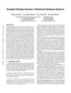
given as input to the model. An operator tree together with a mapping of system processors to operators of the tree constitutes a parallel execution schedule [14]. An example parallel execution schedule is presented in Fig. 1. This shows an execution schedule for a query joining relations A, B and C and computing an aggregate function (e.g. max) over the resulting set of tuples. The execution schedule is typical of Informix XPS, and describes the following sequence of actions. Relation A is scanned and its tuples are used to build a hash table in preparation for joining with B. B is scanned and tuples from it are used to probe the hash table; the resulting join tuples then build a second hash table. C’s tuples are scanned and used to probe the second hash table. Join tuples resulting from the last probe phase are aggregated.

Redistribution of tuples takes place between a scanning and

corresponding building phase in accordance with the requirements of the hash-join algorithm. Arrows between nodes of the schedule represent flow of data as well as timing dependencies. Solid arrows denote blocking. For example, the probing of a hash table with tuples from C can begin only after the hash table has been built – hence the solid arrow between nodes “BUILD A⊗B” and “PROBE C”. Dotted arrows denote pipelined execution.

7

For example, the scanning of tuples from A and their insertion into a hash table can be done in a pipeline (nodes “ SCAN A” and “ BUILD A” ).

Similarly a 3-stage pipeline can be

established for the scanning of tuples from B, probing a hash table with them, and using resulting tuples to build a new hash table (“ SCAN B” , “ PROBE B” and “ BUILD A⊗B” ). Partitioned parallelism is achieved by spreading an operator across multiple machine processors, as specified in the figure. For example, the scanning of A is carried out on PEs 02, as dictated by data placement constraints. Similarly, after redistributing the tuples selected from A, the building of the hash table takes place across the same three PEs. SCAN A PE0,PE1,PE2

BUILD A

SCAN B PE3,PE4

PE0,PE1,PE2

PROBE B PE0,PE1,PE2

BUILD A⊗B PE0,PE1,PE2

SCAN C PE5 PROBE C PE0,PE1,PE2

AGGREGATE A⊗B⊗C PE6, PE7

Fig. 1 Parallel execution schedule

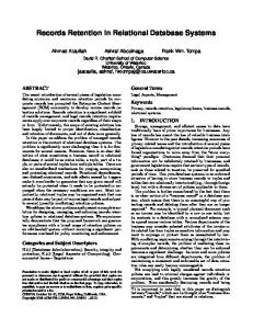
A process akin to “ macro expansion” is then applied to each of the operators at the nodes of the parallel execution schedule. The process transforms each node into a detailed sequence of resource consumption items, termed here a resource usage block. The set of resource usage blocks and their interdependencies (taken from the execution schedule) form the resource usage profile of the query. As an example, consider Fig. 2, which shows the resource usage block corresponding to the “ SCAN A” node of the execution schedule. This represents the process of consecutive fetching of database pages from disc, selecting relevant tuples from the page, and sending them on to another block. This activity is given as a detailed sequence of resource usage. Two types of notation are used in the body of the block (lines 4-28). The first is

8

concerned with the specific uses of individual resources for particular amounts of time. The usage of a particular hardware resource (e.g. processing unit - pu, system support unit - ssu, interconnect - net, disc) for a specified amount of time is represented in italics. Simple examples are lines 5 and 6, where resource ssu is used for time t1 and resource pu for time t2. Line 12 gives an example of a resource (disc0) used for different amounts of time depending on the processing element (PEs 0-2) using the resource. The service time requirements for simple resource usage (ti) are extracted from the particular parallel database architecture modelled. For example, t5, t6, and t7 in line 12 represent the average time spent by disc0 of PE0, PE1,

and PE2 in the process of fetching a data page, while t3 (line 11) is the amount of

service time consumed by the pu resource during the page fetch. 1 2 3 4 5 6 7 8 9 10 11 12 13 14 15

BLOCK: SCAN A HOME: PE0, PE1, PE2 RESOURCE TIME group { ssu t1; pu t2 } PE0:0.0;PE1:1.0;PE2:1.0; loop {PE0:1710;PE1:1501;PE2:1802} { mean_shared_lock_waiting_time; group { pu t3; disc0 {PE0(t5), PE1(t6), PE2(t7)}: } PE0:0.00;PE1:0.76;PE2:0.98; loop {PE0:20;PE1:20;PE2:20} { pu t8;

16 17 18 19 20 21 22 23 24 25 26 27 28 29

group { option { pu t9: 0.6 pu t10: 0.4; }; group { pu t11; ssu t12; net t13 }PE0:0.67;PE1:0.67;PE2:0.67 }0.75 } } END TIME

Fig. 2 Resource usage block

The second type of notation represents templates used to structure simple resource usage items. Templates are represented in bold and are of three types: group, option, and loop. The group template is used to designate a sequence of resource usage items, which has an associated probability of occurring. For example, the group template in lines 21-25 encloses three simple resource items, which represent the resource consumption required for the sending of a selected tuple for processing by the “ BUILD A” operator. The probability associated with this group template is intended to rule out the physical sending across the interconnect of tuples destined for the processor where they are produced. The option template is used to denote choice. It can have a number of branches, each

9

of which has an associated probability and contains a sequence of resource usage items. The grouped items occur together with the given probability. An example of option template use is given in lines 17-20, where the pu resource is used for either time t9 (with probability 0.6) or time t10 (with probability 0.4). The loop template is used to designate repeated use of resources. The consecutive fetching of data pages is conveniently expressed with the loop construct since similar actions are carried out for each fetched page. The loop on line 8 represents the processing of 1710, 1501 and 1802 pages from PE0, PE1, and PE2, respectively. For each page read, a second loop (line 14) is used to represent the processing of individual tuples within the newly read page. 3.2

Mean Resource Response Time Estimation

The aim of the second stage of the method is to estimate the response time of individual hardware resources, given their pattern of use as specified by the resource usage profile. The approach used here is to take the resource usage profile of a query as specifying a queueing network [21,4], and “ solve” the network for resource response time. The network queueing stations are the hardware resources of the machine and are treated as FCFS servers. The transitions among stations are determined by the templates within the resource usage blocks. 1/50

Q1

query Q1 loop 50 resA 32 resB 60 resC 146

32

resA

1

100 1

60

resB 50

query Q2 loop 100 resB 50 resA 100

49/50

99/100

Q2

1 146

resC

1/50

Fig. 3 Queueing network for simple example

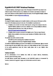
An example of a queueing network for two simple resource usage blocks representing two hypothetical queries is given in Fig. 3.

The pattern of resource consumption is

10

represented as an open queueing network with two customer classes Q1 (solid line) and Q2 (dashed line), as illustrated. Shown are the three resources, the probabilities of transitions among them, and the service times for each customer class and resource. Two difficulties present themselves when working with queueing networks in this context. One concerns the service time requirements at the queueing stations. Typically, exponentially distributed service times with a given mean are assumed. However, in practice assuming non-exponential service times is more realistic. The queueing network is thus composed of non-exponential servers, which renders it a non-product-form network. The second difficulty is to do with the dependencies among resource usage blocks (e.g. pipeline execution and blocking).

This imposes a synchronisation mechanism on the

queueing network, which governs the timing of transitions between stations. There have been numerous studies that address the non-exponential service time problem and lead to analytical approximation techniques [4]. Similarly, many studies are concerned with the synchronisation issues [4]: fork-join queues, blocking queues, etc. We are not aware of any studies, which address both issues simultaneously. The approach used here is to tackle the two problems separately. In this section the first problem is addressed without regard for resource block inter-dependencies (i.e. the transitions between queueing centres are assumed to be of the “ classical” type); the synchronisation issue is dealt with in the next section where overall query response time is estimated from the resource usage profile. The non-product-form nature of the networks due to non-exponential service time requirements means that no exact analytical solutions for the response time or queue length of queueing centres can be found. However, numerous approximation techniques for nonproduct-form networks have been proposed in the literature [4]. In [31] we conduct a comprehensive study of approximation techniques for open multi-class networks. A range of

11

simple models was used and for each model the different approximation techniques were used to predict the response times for varying inter-arrival rates. The results were compared with those obtained from discrete event simulation. From the numerous examples considered in the study, best results were produced when the queueing network was considered to consist of a combination of M/M/1 and M/G/1 queueing centres. This observation was incorporated into a simple heuristic rule, which accounted for all the cases tried. The rule is used to assign the resources of the network with either an M/M/1 or M/G/1 label. In accordance with the assigned label, the queue length or waiting time of each resource can be computed easily from the Khinchin-Pollaczek [21] formula.

The

heuristic rule used is based on the idea of resource dominance, and is summarised below. Definition The dominance of a resource is a weighted average of its utilisation and its relative visit ratio, i.e. vr ( Ri ) dom( Ri ) = 1 × util ( Ri ) + 1 × 2 2 ∑ vr ( R j ) j

where vr(Ri) is the average number of times resource Ri is visited for each arrival from outside. This corresponds to the visit ratio defined in [21] where the reference queue is q0 (the outside world). Since both utilisation and relative visit ratio are numbers in the range 0 to 1, so also is dominance. Although relative visit ratio does not depend on query arrival rate, utilisation does. Thus, the utilisation of each resource must be taken for some particular query arrival rate (e.g. when the bottleneck resource has utilisation of 80%). The heuristic rule is now as follows: (a) Find the dominance of each resource. (b) If there is a single dominant resource, i.e. dom(Ri) > dom(Rj) for all j ≠ i, then according to the squared coefficient of variation of service time for each resource, label the resources as follows:

12

•

label dominant resource Ri as max(M/M/1, M/G/1)

•

label other resources Rj as min(M/M/1, M/G/1)

(c) If there is more than one dominant resource, i.e. dom(Ri1) =…= dom(R in) > dom(Rj) for all j ≠ i1…in then label all resources as min(M/M/1, M/G/1). (d) According to the label, use the Khinchin-Pollaczek formula to compute resource waiting time. For parts (b) and (c) of the rule, the M/G/1 formula collapses into the M/M/1 formula when the squared coefficient of variation of the service time is 1.0; however, if the latter is less than 1.0, max(M/M/1, M/G/1) = M/M/1 whereas if it is greater than 1.0, max(M/M/1, M/G/1) = M/G/1. 3.3

Mean Transaction Response Time Estimation

Given the estimated queue waiting time of individual resources according to the above rule, the response time of the query can be estimated. This process is essentially a traversal of the resource block profile. During the traversal, response time is accumulated according to the structure of the blocks and the dependencies among blocks. In particular, account is taken of the templates within each block (group, option, loop, etc.), the partitioned parallelism, and the blocking or pipeline dependency among blocks.

This is detailed below.

First the

response time estimation within a resource usage block not involved in a pipeline with others is discussed. This is extended to the case of such a block executing in parallel across several nodes (partitioned parallelism). Next, pipelined execution of blocks is considered. Finally, an overall response time for the complete resource usage profile of the query is obtained. 3.3.1

Templates

Within a resource usage block not involved in a pipeline with other blocks and running on a single processor, the response time of a sequence of one or more resource usage items is the sum of their response times. Each of these items may be a simple usage or a template (group, 13

option or loop). The response time of a simple usage involving resource r is the sum of the particular service time and the mean waiting time of the resource, as estimated by the rule. Denote this response time as RT(r). For a group template with probability p (group {usg1;…; usgn} p), the response time is computed as RT ( group ) = p × ( RT (usg1 ) + K + RT (usg n )) . In the case of an option template (option {usg1:p1;…; usgn:pn}),

the

response

time

is

given

by

RT (option) = p1 × RT (usg 1 ) + K + p n × RT (usg n ) . The loop template denotes pipeline execution internal to the block. The response time of a loop usage is computed from the pipeline initialisation time and production time. A simple example of a pipeline is given in Fig. 4 to illustrate the idea. Three resources (resA, resB and resC) are organised in a pipeline that performs 10 iterations. The resources take 3, 4 and 1 unit of time per iteration, respectively. These represent the actual service time added to the mean waiting time for the resource as estimated by the rule; the service times are not shown. This applies to all subsequent examples. The execution pattern is presented on the right hand side. The first iteration completes after 3 + 4 + 1 time units. Thereafter, an iteration completes every 4 time units as determined by resB, the pipeline bottleneck. This time (4 time units) is termed the production time of the pipeline and is the highest response time among the resources in the loop. The time from start to end of an iteration (in this case 3 + 4 + 1 = 8 time units) is termed the pipeline initialisation time. It is equal to the sum of the response times of all resources involved. The response time of a pipeline loop of n iterations is approximated as: RT (loop ) =

∑ rt (r , L) + (n − 1) × rt (bn(res( L), L), L)

r∈res ( L )

where: • L is the set of resource usage items within the body of the loop; • res(U) is the set of resources involved in the set of usage items U;

14

• rt(r, U) is the response time of resource r given its involvement in usage items from U; • bn(R, U) is the bottleneck resource (the one with highest response time) among those in set R given their involvement in usage items from U. resA loop 10 { resA 3; resB 4; resC 1 }

resB

resC

iteration 1st 2nd 3rd

iteration odd even

4th etc.

Fig. 4 Pipelined execution

Informally, the response time is the sum of the initialisation time and the product of (n– 1) and the production time. For the given example the formula evaluates to (3+4+1)+9×4=44 time units. This example is for a very simple loop. Typically, more complicated patterns of resource usage exist within the body of the loop, involving group or option templates. In this case, resource consumption is accumulated for each resource involved in the loop (by rt(r, U) and bn(R, U)) according to the templates and probabilities involved. The production and initialisation times are calculated based on these accumulated quantities. In some cases, such as the resource block shown previously in Fig. 2, one loop template occurs within another. The inner loop is the last template of the outer loop. A simpler example is given in Fig. 5(a). The overall response time depends on the response times of resources from the inner and outer loops and the number of iterations of the inner loop. Suppose the inner loop, considered in isolation, has smaller overall response time than that of the bottleneck resource from the outer loop. In this case, the bottleneck of the outer loop determines the overall response time of the system. Otherwise, the inner loop, of which there are 15 iterations altogether, determines the performance. This type of analysis is carried out

15

in the discussion of pipelined blocks in Section 3.3.3. The same reasoning can be applied here. In order to do so, this case of loop usage is treated as being equivalent to two resource blocks working in a pipeline, as shown in Fig. 5(b). With this representation, the analysis of Section 3.3.3 can be reused. loop 5 { resA t1; resB t2; loop 3 { resC t3; resD t4 } }

loop 5 { resA t1; resB t2 }

loop 15 { resC t3; resD t4 }

(a)

(b)

Fig. 5 Example of loop within a loop

3.3.2

Partitioned parallelism

The home field of a resource usage block specifies the processing elements used to execute the block and thus is an indication of intra-operation parallelism. For example, in Fig. 2, execution is spread over PE0,

PE1

and

PE2.

The total response time of a block is obtained in

two steps. First, the response time of each processing element from the block’s home is calculated by accumulating time for the sequence of resource usage items in the body of the block. This is done following the procedure outlined above. Second, the processing element with the largest accumulated response time is found. This value is the response time of the block. Since all processing elements in its home are running in parallel, the block will complete when the processing element with the longest response time completes. 3.3.3

Pipelined parallelism

A pipeline may span two or three blocks within a query tree, which is typical of the queries used for validation in Section 4. Consider the case of two single-home blocks in a pipeline with one sending tuples and the other receiving them. A simple example of two such blocks is shown in Fig. 6.

PE1

of block1 sends n tuples in a pipeline (in a similar way to the example

in Fig. 4). The sending of a tuple requires work from all three resources resA1, resB1 and 16

resC1. Let t2 be max(t1, t2, t3). The bottleneck resource of this pipeline is thus resB1; the pipeline production time is t2 and the initialisation time is t1 + t2 + t3. Block2 on PE2 receives the n tuples and performs further operations using resources resA2 and resB2.

The

production time of this pipeline is t5. The full processing time needed to receive a tuple (the initialisation time of this loop) is t4 + t5. BLOCK: block1 MODE: independent HOME: pe1

loop n { resA1 t1; resB1 t2; resC1 t3 }

block1

block2

resA1 resB1 resC1 resA2 resB2

T1

BLOCK: block2 MODE: pipeline HOME: pe2

block1

loop n { resA2 t4; resB2 t5 }

T2

Fig. 6 Two blocks in a pipeline

Time T1 in Fig. 6 is the time at which the first iteration of the loop in block1 is complete and the first tuple has been sent to and is about to be received by block2. Similarly, T2 is the time when the last tuple has just been sent and the work needed for its processing in block2 begins. Between times T1 and T2 the sending and receiving process execute together in parallel. The response time of the system depends on the relative speeds of sender and receiver. Let the bottlenecks of the two loops be r1∗ and r2∗ , i.e. bn(res( L1 ), L1 ) = r1∗ and bn(res( L2 ), L2 ) = r2∗ . Since the resources required by the two blocks are disjoint, if the sending process can send its tuples in less time than the receiving one can process them, i.e. rt (r1∗ , L1 ) < rt (r2∗ , L2 ) , then the total time of the system is governed by the speed of the receiver and may be approximated as

∗

∑ rt (r , L1 ) + (n − 1) × rt (r2 , L2 ) +

r∈res ( L1 )

∑ rt (r , L2 ) .

r∈res ( L2 )

Here, L1 and L2 stand for the set of resource usage items in the loops of block1 and

17

block2, respectively. The first component in the formula accounts for the time prior to T1. The second covers the period between T1 and T2, and the third from T2 to the end of execution. For the example this would be (t1 + t2 + t3) + (n - 1) × t5 + (t4 + t5). On the other hand, if the receiving process takes less time than the sending process, i.e. rt ( r1 , L1 ) > rt ( r2 , L2 ) , *

*

then the total time of the system is governed by the sender: ∗ ∑ rt (r , L1 ) + (n − 1) × rt (r1 , L1 ) +

r∈res ( L1 )

∑ rt (r , L2 )

r∈res ( L2 )

If the resources required by the two blocks are not disjoint, then the calculation of the production time of each loop must take into account any usage of shared resources taking place in the other loop. Suppose the bottleneck resources of the two loops are r1∗ and r2∗ , i.e. bn(res( L1 ), L1 U L2 ) = r1∗ and bn(res( L2 ), L2 U L1 ) = r2∗ . Note that the bottlenecks are determined taking into account resource consumption from both loops. In the case when r1∗ ≠ r2∗ a similar analysis to that for the case of disjoint resources applies. In other words, if rt (r1∗ , L1 U L2 ) < rt (r2∗ , L2 U L1 ) , then the response time of the system is determined by that of the receiver and may be approximated as: ∗

∑ rt (r , L1 ) + (n − 1) × rt (r2 , L2 U L1 ) +

r∈res ( L1 )

∑ rt (r , L2 )

r∈res ( L2 )

In the case of a slower sender, the overall response time is determined by the sender’s production time

∗ ∑ rt (r , L1 ) + (n − 1) × rt (r1 , L1 U L2 ) +

r∈res ( L1 )

∑ rt (r , L2 ) .

r∈res ( L2 )

If r1∗ = r2∗ (i.e. the bottleneck is a shared resource for the two loops), the response time of the sender/receiver system is approximated as the sum of the response times of the two loops:

∗ ∑ rt (r , L1 ) + (n − 1) × rt (r , L1 ) +

r∈res ( L1 )

∗ ∗ ∗ ∗ ∑ rt (r , L2 ) + (n − 1) × rt (r , L2 ) , where r = r1 = r2 .

r∈res ( L2 )

The idea that the overall time of a sender/receiver system is determined by the slower of the two can also be extended to apply to the case of multiple senders and receivers. This represents the case of a block with a multiple processor home sending tuples to another block 18

executing on multiple processors, with senders and receivers working in parallel. Typically, redistribution of tuples takes place between the two blocks and different numbers of tuples may be sent/received by different sending/receiving loops, as illustrated in Fig. 7. The total time of this system is determined by the slowest of all sending and receiving loops. BLOCK:

block1

HOME:

pe1 loop 16 { resA1 1; resB1 3; resC1 4 } BLOCK:

HOME:

pe2 loop 8 { resA2 2; resB2 6; resC2 4 }

block2

HOME:

pe1 loop 4 { resD1 1; resB1 2 }

HOME:

pe3 loop 20 { resA3 4; resB3 5; resC3 2 }

Fig. 7 Multi-home blocks in a pipeline.

First, all sending loops are analysed to determine the slowest one, as follows. Consider sending loop LS. Suppose there is no receiving loop LR sharing resources with LS and let

bn(res( LS ), LS ) = rL∗S . The response time of LS can be approximated as before: RT ( LS ) =

∗

∑ rt (r , LS ) + (iter ( LS ) − 1) × rt (rLS , LS )

(1)

r∈res ( LS )

where iter(L) is the number of iterations in loop L. If the set of processors on which the sending and receiving blocks operate are not disjoint (as in Fig. 7), a receiving loop, LR, may share resources with LS. In this case, let rL∗S be the bottleneck resource of LS, taking into account any shared use. Formally,

rL∗S = BN (res( LS ), ( LS , iter ( LS )), ( LR , iter ( LR ))) ,

(2)

where BN(res(L1), (L1, n1), (L2, n2)) returns resource ri ∈ res(L1) such that n1 × rt(ri, L1) + n2 × rt(ri, L2) > n1 × rt(rj, L1) + n2 × rt(rj, L2) for all j ≠ i. Then the response time can be approximated according to the following formula, which takes into account the use of rL∗S

19

within both loops: RT ( LS ) =

∑ rt (r , LS ) + (iter ( L S ) − 1) × rt (rLS , L S ) + *

(3)

r∈res ( LS )

iter ( L R ) × rt (rL*S , L R ) The same analysis can be carried out on each receiving loop, LR, in order to obtain an estimation of its response time, RT(LR). The overall response time of the system of senders and receivers is approximated as follows. Let LS and LR be the sending and receiving loops with the highest response times as determined by the above procedure. Let their bottlenecks be rL∗S and rL∗R , respectively. Suppose that rL∗S ≠ rL∗R . If RT(LS) < RT(LR) then: RT = avg( LS i

∑

r∈res ( LS i )

rt (r , LSi )) + RT ( L R )

(4)

On the other hand, if RT(LS) > RT(LR), then: RT = RT ( LS ) + avg( L Ri

∑

r∈res ( LR i )

(5)

rt (r , LRi ))

In the above two formulae, the average initialisation time of all sending/receiving loops is used to account for the time needed for the first/last tuple to be sent/received. If, however, rL∗S = rL∗R , then RT =

∗

∑ rt (r , LS ) + (iter ( LS ) − 1) × rt (rLS , LS ) +

r∈res ( LS )

∗

∑ rt (r , LR ) + (iter ( LR ) − 1) × rt (rLR , LR )

r∈res ( LR )

Consider the example given in Fig. 7, which can be used to illustrate the process of estimating the response time according to the above analysis. Consider first each sending loop. The loop on PE1 shares a resource (resB1) with the receiving loop on the same node and therefore (2) and (3) are used to calculate the response time. The bottleneck resource of this loop ( rL∗S ), calculated according to (2), is the shared resource resB1, since its combined usage within both loops is greater than those of the three other non-shared resources (resA1,

20

resC1 and resD1). The response time of the sending loop can be calculated from (3) as (1+3+4)+(16–1)×3 + 4×2 = 61. The sending loop on PE2 does not share any resource usage, and its response time can be calculated from (1). The bottleneck resource of this loop is resB2 (with response time of 6) and therefore the response time of this sending loop is (2+6+4) + (8-1)×6 = 54. Consider next the receiving loops. Their response times are estimated in a similar way. The receiving loop on PE3 does not share resources with a sending loop and evaluates (via (1)) to (4+5+2) + (20–1)×5 = 106. The receiving loop on PE1, however, shares resource resB1 with the sending loop on the same node. Resource resB1 is the bottleneck of this loop and the loop’s response time was computed above as 61. Now consider the sending and receiving loops with the highest response times. These are the sending loop on PE1 with response time of 61 and bottleneck resB1 and the receiving loop on PE3 with response time of 106 and bottleneck resB3. Since the two bottlenecks are different, and the receiving loop has a higher response time, the overall response time of the system may be approximated according to (4) as avg(1+3+4, 2+6+4) + 106 = 10 + 106 = 116. This approach can be extended to a pipeline of three or more stages, as follows. First, the slowest stage of the pipeline is identified. This stage could be the initial sending stage of the pipeline, an intermediate sending/receiving stage, or the final receiving stage.

The

response time of each stage of the pipeline is determined by the response time of the slowest sending/receiving loop within the stage, taking account of shared resource usage as needed. Then, the total time of the pipeline is approximated as the total time of the slowest stage, plus the average initialisation times within each of the remaining phases, in a similar way to that explained above. 3.3.4

Overall response time

Thus far, the focus has been on estimating response time for various stages of the execution

21

schedule of the query. The response time for the query as a whole can be determined as follows. The pipeline dependencies among blocks are considered in order to determine which blocks can be analysed together as a single pipeline. The full dependencies are considered to establish when a block (or group of blocks engaged in a pipeline) must wait for other blocks to complete before it can begin execution. Consider the example execution schedule from Fig. 1. The overall response time of the query is the sum of the response times of three distinct phases within the execution schedule. The first phase is the two-stage pipeline involving blocks ‘SCAN A’ and ‘BUILD A’. The second stage consists of the three-stage pipeline involving blocks ‘SCAN B’, ‘PROBE B’ and ‘BUILD A⊗B’. The final phase is the three-stage pipeline involving blocks ‘SCAN C’, ‘PROBE C’, and ‘AGGREGATE A⊗B⊗C’.

4

Validating the Technique

The ICL Goldrush MegaServer [34,35] is a parallel platform developed as a back-end database server to host several different database systems (Ingres, Oracle, Informix). In this section results from the validation of the model are discussed. 4.1

Goldrush and Informix XPS

The basic Goldrush hardware architecture consists of a number of Processing Elements (PEs) and Communication Elements (CEs) linked by a high speed Deltanet network. Each

PE

is

connected to its own disc storage subsystem and runs a version of the UNIX operating system and DBMS code. A

CE

provides external links for Goldrush to clients via LANs. The

particular Goldrush configuration used here has 1

CE,

8

PEs,

6 discs per

PE

and a cache of

16MBytes on each PE. This type of architecture is an ideal platform for the shared-nothing Informix Extended

22

Parallel Server (XPS) [20]. It contains a set of internal components called co-servers, which are installed on each of the Goldrush on a given

PE.

PEs

of Goldrush. A co-server provides a user entry point to

Locks on data items and all data processing are managed locally

within each co-server. Where deemed suitable, single queries are broken into subtasks and processed concurrently by threads within a single co-server and across co-servers. Data can be partitioned across discs and PEs so that parallel I/O operations can take place. The system can detect that certain partitions are irrelevant for a particular query and would not consider them when executing the query. 4.2

Tables

The experiments detailed in this section are carried out on a subset of the AS3AP benchmark [32] tables. In particular, the Uniques relation is used, the structure of which is given in Table 1. A number of variations of this relation were produced as shown in Table 2. Attribute name key int signed float double decim date code name address

Attribute type integer(4) integer(4) integer(4) real(4) double(8) numeric(18,2) datetime(8) char(10) char(20) varchar(20)

Name un80 un30k un90k un120k un270k un540k

Rows 80 30,000 90,000 120,000 270,000 540,000

Placement 1 disc 1 disc 1 disc 1 disc 1 disc of each PE 1 disc of each PE

Table 2 Uniques relations used

Table 1 Attributes of Uniques relations

Un270k and un540k are fragmented into 8 fragments by a simple hash function on the key primary key attribute with one hash fragment placed on a single disc of each of the PEs. Each tuple has a unique value for attributes key and int. Attribute signed, however, is modified from the benchmark specification so that for each relation tuples have signed values in the range 1 to 10 with an equal number of tuples for each value. Scans involving tables placed on one PE are not parallelised. Those involving tables un270k and un540k, however,

23

are performed in parallel by all co-servers containing the table data. 4.3

Queries

A number of different queries, classified in the following groups, were considered: Simple select-project-aggregate queries. This group of queries exercises the ability of the method to work for the simple relational operations select, project and aggregate. Different tables (X), predicates (Y) and aggregation operators (max, count, etc) are used, as shown in Fig. 8(a). Simple hash-join queries. Each of these queries (Fig. 8(b)) finds the maximum value of the int attribute from the result of a join of un80 with the other Uniques tables where the int values are the same. Each of the other tables contains the tuples of un80 so that the size of the resulting join is 80 tuples. The query employs a hash-join algorithm, which builds a hash table across all co-servers using un80 and subsequently probes this with the tuples from X. (1)

select max(int) from X where key > 0;

select max(un80.int) from un80, X where un80.int = X.int

(2)

select max(int), min(int) from X where Y;

X = un30k, un90k, un270k, un540k

select max(int), min(int), avg(int), count(*) from X where Y;

select max(int) from un30k where int > (select max(key) from un30k where signed not in (1,3,5));

(3)

(b)

X = un30k, un90k, un270k, un540k; Y = “ signed not in (1)” , “ signed not in (1, 3, 5)”

max1 = select max(key) from un30k where signed not in (1,3,5); select max(int) from un30k where int > max1 (c)

(a)

Fig. 8 Queries used for validation

Simple nested query and equivalent non-nested version. This is a simple example of the use of a sub-query. The sub-query is used to return the maximum value of the key attribute from a subset of the tuples of un30k. This value is then used in the predicate of the

24

outer query. Note that this is not a correlated sub-query, and the execution plan indicates that Informix executes the sub-query first followed by the outer query. An equivalent “ flat” formulation of the query was also considered, as shown in Fig. 8(c). The sub-query executes first as an independent query. Following it, a second query uses its result to compute the maximum int value. Although equivalent in their execution, the two queries have different response time characteristics, as discussed briefly in Section 4.5. A union query. This query, shown in Fig. 9(a) illustrates the execution of the Informix union operator when there is opportunity for parallelism. The query groups together the maximum int values from tables un30k and un270k. It was expected that some form of parallelism would be used when executing the query. However, the execution plans indicate a sequential execution, with un30k scanned first, followed by the scanning of un270k, and followed by the union operator. To investigate this, the same query was executed with two un90k tables, specifically created on different processing elements and discs of Goldrush. Even in this case, where clearly the query can execute in half the time if the two relations are scanned in parallel, Informix chooses to perform the two scans in sequence. A three-way hash-join. The execution schedule of this query was discussed in Section 3.1 and shown in Fig. 1. The query is shown in Fig. 9(b). Tables A, B and C, used in the discussion, correspond to un80, un90k, and un30k, respectively. select max(int) from un30k where int > 0 union all select max(int) from un270k where int > 0

select max(un30k.int), count(un30k.int) from un90k, un30k, un80 where un90k.key = un30k.key and un30k.key = un80.key (b)

(a) Fig. 9 Queries used for validation

4.4

Taking Measurements

Calibration of the model required running a carefully constructed set of queries in order to

25

estimate the cost of basic operations. The parallelised query execution plans produced by the optimiser were used to determine the way in which queries were broken down by the system and what basic operations were involved. Their costs were then obtained using the Informix XPS performance measuring tool onstat. Once this was complete, a transaction generator was created to emulate a parallel database system workload with many users independently querying the data. It was used to fire queries from the communication element (CE) to a given co-server at a specified rate. Two generators were created. The first fired transactions with constant inter-arrival times and was used to determine the arrival rate for which the maximum throughput of the machine can be achieved. The throughput was computed by dividing the number of completed transactions by the time between the start time of the first transaction and the end time of the last one. Initially, the measured throughput is equal to the arrival rate at which the queries are fired. As the arrival rate is increased, a value is reached beyond which the measured throughput does not increase further. This is taken to be the maximum system throughput. The second version of the transaction generator fired transactions with exponentially distributed inter-arrival times and was used to obtain transaction response times. The highest arrival rate used for the exponential generator was equal to 80% of the rate at which the maximum throughput (determined using the deterministic generator) was achieved. For each arrival rate the generator was set to fire transactions until 100 transactions were fired. The response time of each query was recorded, and the average was formed to compare against the value estimated by the analytical method. At the higher arrival rates, when queues would build quickly and the system would take longer to settle into a steady state, more than 100 queries were run when needed. Note that due to the good repeatability of measurements obtained from Informix, it was generally found necessary to repeat experiments no more than three times.

26

4.5

Results

Simple select-project-aggregate queries.

Fig. 10 shows the maximum throughput

prediction against actual measured throughput for one of the queries. The x-axis represents arrival rate and the y-axis – throughput. The prediction produced by the tool is a single figure: the maximum possible throughput, which is independent of the arrival rate. The predicted maximum throughput is higher than the one achieved by the system. This can be attributed to additional operating system overhead for which no account has been taken in the model, or to inaccuracies in the measured basic costs. Despite this, the predicted maximum throughput is an acceptable upper limit of the achieved maximum system throughput. 45

0.117497

0.11

40

0.1

35

0.09 measured predicted maximum

0.08 0.07 0.06

response time (sec)

throughput (trx/sec)

0.12

30 25

measured

20

predicted

15 10

0.05

5 0.04 0.04

0.06

0.08

0.1

0 0.01

0.12

arrival rate (trx/sec)

0.03

0.05

0.07

0.09

0.11

arrival rate (trx/sec)

Fig. 10 Throughput for type (1) query on un90k

Fig. 11 Response time for type (1) query on un90k

The response time predictions for this query are shown in Fig. 11. The x-axis measures arrival rate, while the y-axis represents the response time. The prediction is accurate to within 10% for the entire range of arrival rates. All the experiments reported here were performed with the data present in cache. By comparison, consider a query of type (1) using table un120k, for which all data pages are read from disc. The results from two experiments performed are presented in Table 3. The arrival rates of the experiments correspond to 40% and 80% of the maximum throughput. experiment 1 2

arrival rate (trx/sec) 0.03 0.06

response time (sec) measured predicted 24.9 23.9 74.8 83.4

relative error (%) -4.0 11.5

Table 3 Results for query reading pages from disc

Simple hash-join queries. Fig. 12 shows the maximum throughput prediction against 27

actual measured throughput for this query on table un540k. Again the tool’ s prediction is higher than the achieved maximum throughput. Fig. 13 shows the response time prediction compared with measured response time. 50

0.16 0.15

45

0.148249

40

0.13 0.12 measured predicted maximum

0.11 0.1 0.09

response time (sec)

throughput (trx/sec)

0.14

35 30

15 10

0.07

5

0.08

0.1

0.12

0.14

0 0.02

0.16

predicted

20

0.08

0.06 0.06

measured

25

0.04

arrival rate (trx/sec)

0.06

0.08

0.1

0.12

0.14

arrival rate (trx/sec)

Fig. 12 Throughput for simple hash-join query on un540k

Fig. 13 Response time for simple hash-join query on un540k

Simple nested query and equivalent non-nested version. The graph in Fig. 14 shows the response time prediction and the corresponding measured values for the non-nested version of this query. The tool compares better with the non-nested query. The nested version of the query seems to involve extra resource usage, which can be attributed to the query optimiser ‘un-nesting’ the original query. The performance model does not currently account for this type of activity. Three-way hash-join query. The response time results obtained for this query are

18

50

16

45

14

40

12 10

measured

8

predicted

6

response time (sec)

response time (sec)

presented in Fig. 15. The predicted values are within 15% of the measured values.

35 30

15 10

2

5

0

0.05

0.1

0.15

0.2

predicted

20

4

0

measured

25

0 0.01

arrival rate (trx/sec)

0.03

0.05

0.07

0.09

0.11

arrival rate (trx/sec)

Fig. 14 Response time for non-nested version of query

Fig. 15 Response time for a three-table hash join query

The results of the response time prediction method for all queries are summarised in Table 4. The table gives the number of experiments and indicates the magnitude of the relative percentage error computed from the predicted and measured response time for each

28

query category. experiments 0% - 60% max throughput 70% - 80% max throughput no. of no. with no. with no. with no. of no. with no. with no. with exp. err. below err. 10err. 20exp. err. below err. 10err. 2010% 20% 30% 10% 20% 30% 11 9 2 5 4 1 1 1 1 1 21 17 4 9 5 4 15 3 12 8 3 5 8 8 6 3 3 5 4 1 11 6 5 3 3 5 5 3 3 2 2 -

Query

type 1 type 1 (from disc) type 2 type 3 simple hash-join non-nested union triple join

Table 4 Summary of results

The experiments are divided into two groups depending on the value of the arrival rate for the experiment. The first category is for arrival rates that are up to and including 60% of predicted maximum throughput, while the second is for rates between 70% and 80%. A two-query application. The results of a two-query application are also presented. The two chosen queries are a type (3) query on relation un30k with predicate ‘signed not in (1, 3, 5)’ and a type (1) query on relation un30k (see Fig. 8). The queries are assigned different frequencies: 70% for the first and 30% for the second.

The measured and

approximated response times of the two queries are presented in Fig. 16 and Fig. 17. There is

16

18

14

16

12

14

10 measured

8

predicted

6 4

response time (sec)

response time (sec)

a reasonable match between the approximation and the measured values.

12 10

measured

8

predicted

6 4

2

2

0

0 0

0.05

0.1

0.15

0.2

0.25

0.3

0

arrival rate (trx/sec)

0.1

0.15

0.2

0.25

0.3

arrival rate (trx/sec)

Fig. 16 Response time of first query

5

0.05

Fig. 17 Response time of second query

Conclusions

In this paper an analytical technique is presented for response time estimation of queries executing within a shared-nothing parallel database management system. This technique

29

deals with the problem of non-exponential servers as well as with dependencies such as pipelining. It is based on a heuristic approach, used to obtain a better approximation of the behaviour of a network of non-exponential servers as used in parallel database systems than other approximation techniques.

The techniques were validated by comparing their

predictions against actual performance measurements on a parallel database system. The experiments indicate that the estimated and measured quantities are in reasonably good agreement. In particular, the predicted maximum throughput is typically higher than the measured maximum throughput by up to 15%. A possible explanation for this is additional resource consumption due to activity by non-DBMS processes or the operating system itself. Such activity is not accounted for within the models at present.

Despite this, the

approximation to the maximum system throughput is acceptable. The experiments also show that the response time approximation technique produces reasonably good results. In particular, a total of 114 separate experiments were performed involving different transactions and arrival rates. In 96 of the experiments (over 84%) the relative error is less than 20%. In half of these, the error is less than 10%. For the remaining 18 experiments, the highest error is under 30%. Generally, the error is smaller for the lower transaction arrival rates and increases as the arrival rate is increased. Acknowledgements The authors acknowledge the support received from the UK Engineering and Physical Sciences Research Council (EPSRC) under the PSTPA programme (GR/K40345) and from the Commission of the European Union under the Framework IV programme (Mercury project). They also wish to thank Arthur Fitzjohn and Monique Mitchell of ICL.

30

References [1]

L. Anciano, N.N. Savino, J.A. Corbacho and R. Puigjaner, “ Extending SMART2 to predict the behaviour of PL/SQL-based applications” , in Proc. of 10th Int. Conf. on Modelling Techniques and Tools for Computer Performance Evaluation (Tools’98), Palma de Mallorca, Spain, pp.292-305, 14-18 Sept. 1998.

[2]

B. Bergsten, M. Couprie and P. Valduriez, “ Prototyping DBS3, a shared-memory parallel database system” , Proc. of the 1st Int. Conf. on Parallel and Distributed Information Systems, Miami Beach, FL, USA, p.226-234, 4-6 Dec 1991.

[3]

BEZ Systems Inc., “ BEZPlus for NCR Teradata and Oracle environments on MPP machines” , http://www.bez.com/software.htm, 1999.

[4]

G. Bolch, S. Greiner, H. de Meer and K.S. Trivedi, “ Queueing networks and Markov chains: modelling and performance evaluation with computer science applications” , John Wiley & Sons Inc., 1998.

[5]

H. Boral, W. Alexander, L. Clay, G. Copeland, S. Danforth, M. Franklin, B. Hart, M. Smith and P. Valduriez, “ Prototyping Bubba, a highly parallel database system” , IEEE Transactions on Knowledge and Data Engineering, vol.2, no.1, pp.4-24, Mar 1990.

[6]

J. Boulos and D. Boudigue, “ An application of SMART2: a tool for performance evaluation of relational database programs” , in Joint proc. of 8th Int. Conf. on Modelling Techniques and Tools for Computer Performance Evaluation and 8th GI/ITG Conf. on Measuring, Modelling and Evaluating Computing and Communication Systems, Heidelberg, Germany, pp.11-25, 20-22 Sept. 1995.

[7]

A. Dan, “ Performance Analysis of Data Sharing Environments” , The MIT Press, 1992.

[8]

A. Dan and P. Yu, “ Performance analysis of buffer coherency policies in a multisystem data sharing environment” , IEEE Trans. On Parallel and Distributed Systems, vol. 4, no. 3, pp. 289-305, March 1993.

31

[9]

E. Dempster, N. Tomov, J. Lu, C. Pua, M. H. Williams, A. Burger, H. Taylor and P. Broughton, “ Verifying a Performance Estimator for Parallel DBMSs” , in Proc. of 4th Int. Euro-Par Conf. (Euro-Par ‘98 Parallel Processing), Southampton, UK, pp. 126135, September 1-4, 1998.

[10]

D. Dewitt, S. Ghandeharizadeh, D. Schneider, A. Bricker, H.I. Hsiao and R. Rasmussen, “ Gamma database machine project” , IEEE Transactions on Knowledge and Data Engineering, vol.2, no.1, pp.44-62, Mar 1990.

[11]

R. Eberhard, IBM Corp. “ DB2 Estimator for Windows” , http://www.software.ibm.com/data/db2/os390/estimate, 1999.

[12]

T. Foxon, M. Garth and P. Harrison, “ Capacity planning in client-server systems” , Journal of Distributed Systems Engineering, vol. 3, pp. 32-38, 1996.

[13]

S. Ganguly, W. Hasan and R. Krishnamurthy, “ Query optimisation for parallel execution” . In Proc. of the 1992 ACM SIGMOD Int. Conf. on Management of Data, San Diego, California, pp. 9-18, June 1992.

[14]

M. Garofalakis and Y. E. Ioannidis, “ Multi-dimensional resource scheduling for parallel queries” , In Proc. of the 1996 ACM SIGMOD Int. Conf. on Management of Data, Montreal, Canada, pp.365-376, June 1996.

[15]

M. Garth, “ Capacity planning for parallel IT systems” , The Computer Bulletin, vol. 8, no. 5, pp. 16-18, November 1996.

[16]

M. Garth, “ Modelling parallel architectures” , Metron Technology white paper, http://www.metron.co.uk/papers.htm#PARA, 1996.

[17]

G. Graefe, “ Parallelizing the volcano database query processor” , Proc. 35th IEEE Computer Society Int. Conf., pp.490-493, 26 Feb - 02 Mar 1990.

[18]

W. Hong and M. Stonebraker, “ Optimization of parallel query execution plans in XPRS” , Distributed and Parallel Databases, vol.1, no.1, pp.9-32, Jan 1993.

32

[19]

H. Hsiao, M. Chen and P. Yu, “ On parallel execution of multiple pipelined hash joins” , In Proc. of the 1994 ACM SIGMOD Int. Conf. on Management of Data, Minneapolis, Minnesota, pp.185-196, May 1994.

[20]

Informix Software Inc., “ Informix-OnLine extended parallel server for loosely coupled cluster and massively parallel processing architectures” , Informix White Paper, http://www.informix.com, 1998.

[21]

M. Molloy, “ Fundamentals of performance modelling” , Macmillan Publishing Company, 1989.

[22]

Platinum Technology, “ Proactive performance engineering” , Platinum Technology white paper, http://www.softool.com/products/ppewhite.htm, 1999.

[23]

S. Salza and M. Renzetti, “ Performance modelling of parallel database systems” , Informatica, vol.22, pp.127-139, 1998.

[24]

S. Salza and R. Tomasso, “ A modelling tool for the performance analysis of relational database applications” , In Proc. 6th Int. Conf. on Modelling Techniques and Tools for Computer Performance Evaluation, pp.323-337, 1992.

[25]

SES Inc., “ Solutions for information systems performance” , http://www.ses.com/Solution/IS.html, 1999.

[26]

K. Sevcik, “ Data base system performance prediction using an analytical model” , In Proc. of the 7th Int. Conf. on Very Large Data Bases, Cannes, France, pp. 182-197, September, 1981.

[27]

G. Sigalov and B. Zibitsker, “ Performance evaluation of database computers with high level of parallel processing” , In Proc.of the 19th Int. Conf. for the Management and Performance Evaluation of Enterprise Computing Systems, San Diego, California, pp. 1100-1109, December 1993.

33

[28]

M. Spiliopoulou and J. C. Freytag, “ Modelling the dynamic evolution of system workload during pipelined query execution” , Technical Report ISS-20, Institut für Wirtschaftsinformatik, Humboldt-Universität zu Berlin, Germany, 1995.

[29]

M. Spiliopoulou and J. C. Freytag, “ Modelling resource utilisation in pipelined query execution” , in Proc. of 2nd Int. Euro-Par Conf., Lyon, France, pp. 872-880, 26-29 Aug, 1996.

[30]

M. Spiliopoulou, M. Hatzopoulos and Y. Cotronis, “ Parallel optimization of large join queries with set operators and aggregates in a parallel environment supporting pipeline” , IEEE Trans. On Knowledge and Data Engineering, vol. 8, no.3, pp.429445, June 1996.

[31]

N. Tomov, E. Dempster, M. H. Williams, P. King and A. Burger, “ Approximate estimation of transaction response time “ , The Computer Journal, to appear, 1999.

[32]

C. Turbyfill, C. Orji and D. Bitton, “ AS3AP: an ANSI SQL standard scaleable ad portable benchmark for relational database systems” , in J. Gray (ed.), The benchmark handbook for database and transaction processing systems, 2nd edition, pp. 317-357, 1993.

[33]

C. Walton, A. Dale and R. Jenevein, “ A taxonomy and performance model of data skew effects in parallel joins” , In Proc. of the 17th Int. Conf. on Very Large Data Bases, Barcelona, Spain, pp.537-548, September 1991.

[34]

P. Watson and G. Catlow, “ The architecture of the ICL Goldrush MegaServer” , ICL Systems Journal, vol. 10, no. 2, http://www.icl.com/sjournal/v10i2/v10i2a1.html, November 1995.

[35]

P. Watson and T. Robinson, “ The hardware architecture of the ICL Goldrush MegaServer” , ICL Systems Journal, vol. 10, no. 2, http://www.icl.com/sjournal/v10i2/v10i2a2.html, November 1995.

34

[36]

P. Watson and P. Townsend, “ The EDS parallel relational database system” , in P. America (ed.), Proc. of Workshop on Parallel Database Systems, Noordwijk, the Netherlands, pp. 149-166, Sept. 1991.

[37]

M. H. Williams, E. W. Dempster, N. T. Tomov, C. S. Pua, H. Taylor, A. Burger, J. Lu and P. Broughton, “ An analytical tool for predicting the performance of parallel relational databases” , Concurrency: Practice and Experience, to appear 1999.

[38]

S. Zhou, M.H. Williams and H. Taylor, “ Practical throughput estimation for parallel databases” , Software Engineering Journal, vol.11, no.4, pp.255- 263, Jul 1996.

35