Practical Usage of Algorithmic Probability in Pattern

Practical Usage of Algorithmic Probability in Pattern Recognition Alexey S. Potapov AIDEUS and National Research University of Information Technology, Mechanics and Optics, Russia [email protected] Abstract Solomonoff universal induction based on Algorithmic Probability (ALP) can be considered as the general theoretical basis for machine learning and, in particular, pattern recognition. However, its practical application encounters very difficult problems. One of them is incomputability caused by usage of the Turing-complete solution space. The Minimum Description Length (MDL) and the Minimum Message Length (MML) principles can be considered as simplified derivations of ALP applied to Turing-incomplete solution spaces. The MDL and MML principles have been successfully used to overcome overlearning and to enhance different pattern recognition methods including construction of nonlinear discrimination functions, support vector machines, mixture models, and others. However, restriction of the solution space is not the only simplification in the MDL/MML approaches. All possible models of data are used to calculate ALP, while the only one best model is selected on the base of the MDL/MML principle. In this chapter, the possibility to utilize Turingincomplete version of ALP in the practical tasks of pattern recognition is considered. This gives theoretically and experimentally grounded approach to use “overcomplex” models (similar to compositions of classifiers or mixtures of experts) without the risk of overlearning, but with better recognition rates than that of minimum description length models. It is impossible to sum over all models even in Turing-incomplete model spaces. Thus, it is necessary to select some number of models, which should be taken into account. These models can correspond to different extrema of the MDL criterion. For example, if models can have different number of parameters than the best model for each number of parameters can be taken into consideration. Models constructed on some subsets of a training set can be used for calculating ALP in the case of families of models with fixed number of parameters. Some concrete applications of the ALP-based approach are considered. Its difference from finite mixtures and possible connection with boosting are discussed. 1. Introduction Many different pattern recognition methods exist. This diversity is partially caused by the variety of recognition tasks. However, another reason consists in absence of really comprehensive theory of pattern recognition. Even the most mathematically sound methods and theories contain heuristic elements. The problem of overlearning (overfitting) is one of negative consequences of the insufficient theoretical foundations. Pattern recognition tasks can be interpreted as particular tasks of inductive inference, which consists in search for regularities in observation data (in construction of models of data sources). Methods of inductive inference contain such general components as the model space, decision criterion, optimization or search algorithm. Methods of pattern recognition also include these components in explicit or implicit form. Any negative effect in pattern recognition is the result of selecting an inappropriate model, because of bad criterion, narrow model space or weak search algorithm. The overlearning effect is especially connected with the decision criterion. One of the most widely accepted correct criteria is Bayes’ criterion. However, its usage encounters the well-known problem of prior probabilities [1]. Theory of probability allows one to infer posterior probabilities from prior probabilities, but doesn’t tell

us, how to introduce the very initial probabilities. Different heuristic techniques or semi-theoretical criteria are frequently introduced. For example, overlearning of artificial neural networks is typically prevented by restricting the training time. The most common observation consists in the fact that more complex models should be penalized, because they have more possibilities to fit the data. Such particular criteria as An Information Criterion [2] or Bayesian Information Criterion [3] are well-known. Similar ideas are summarized in the Minimum Description Length (MDL) [4] and Minimum Message Length (MML) [5] principles, which state that the best model to describe the data is the model that provides the minimum value of the sum of the length of the model and the length of the data described with the help of this model. The description length of the encoded data is usually estimated as its negative log likelihood. In practice, the length of the model is calculated using some heuristic coding scheme. For example, if the model is parametric than its length will be proportional to the number of parameters and the number of bits necessary to encode each parameter. Not only does this approach allow for successful practical applications (e.g. [6]–[8]), but also it has strong basis in algorithmic information theory, in which the notion of probability is derived from the amount of information defined on the base of pure combinatorial considerations. However, incorrect generalization is not necessarily accompanied by overlearning. It can be caused simply by absence of the appropriate model in the used model space. Algorithmic information theory also provides us the most wide model space. This is the Turing-complete model space that contains all algorithms as models of possible data sources. Usage of the Turing-complete model space with prior probabilities defined by lengths of algorithms results in the universal induction/prediction method [9, 10] based on Algorithmic Probability (ALP). Existing practical methods are limited in their generalization capabilities, because they rely on the restricted model spaces, which don’t contain all possible regularities. Unfortunately, direct search in the Turing-complete model space is computationally implausible. The representational MDL (RMDL) principle was recently introduced [11] as an extension of the MDL principle that makes possible to take into account dependence of the model optimality criterion from prior information given in data representation. The RMDL principle gives criteria for automatic optimization of data representations, and partially bridges the gap between the theoretically ideal induction methods based on algorithmic complexity and practical applications of the MDL principle relied upon heuristic coding schemes. Completeness of the model space is the essential issue, but there is another difference between the MDL principle that serves for selecting one best model and ALP that implies the usage of all possible models simultaneously [10]. Thus, it would be interesting to consider possible practical versions of ALP or to extend the practical MDL methods with the use of multiple models. In this chapter, some methodological issues of adoption of Bayes’ and Minimum Description Length criteria will be overviewed, and then techniques for the practical usage of Algorithmic Probabilities will be investigated. 2. Bayes’ criterion One of the most widely used mathematical criteria in inductive inference is based on Bayes’ rule:

P ( H ) P( D | H ) . (1) P( D) where P(H | D) is the posterior probability of the model H with the given data D; P(H) and P(D) are the prior probabilities, and P(D | H) is the likelihood of the data D with the given model H. Bayes’ rule can be directly applied to the classification problem. Let D be one pattern, and H be one of the classes. The most probable class for the given pattern can be easily selected maximizing P( H | D) =

2

P(H | D), if the probability density distribution P(D | H) of patterns within each class and the unconditional probabilities P(H) are known. Learning in statistical pattern recognition consists in inducing probability distributions on the base of some training set {di, hi}, where di is the i-th pattern, and hi is its class label. The prior probabilities P(H) can be estimated from frequencies of each class in the training set. The distribution P(D | H) should be represented as an element of some family P(D | H, w), where w is an indicator (e.g. parameter vector) of specific distribution. Using Bayes’ rule and supposing independence of patterns one can obtain: P(w )∏ P(di | hi , w ) i P(w | D) = . (2) P( D) The values of P(di | hi, w) can be explicitly calculated for the specific distribution defined with w. However, there is a problem with evaluation of the prior probabilities P(w). In order to specify these probabilities correctly one needs many training sets, for each of which true probability should be known. It is impossible, because such true probabilities are unknown even for human experts, who construct training sets. Many researchers prefer to ignore prior probabilities and to use the maximum likelihood (ML) approach. The same result will be obtained if one supposes that the prior probabilities are equal. This supposition is evidently incorrect, because the prior distributions in the case of infinite model spaces become non-normalized. In practice, it leads to the overlearning problem. Consider mixture Gaussian models as an example. The likelihood of data will be maximized for the maximum number of components in the mixture leading to the degenerated distribution. The same overfitting effect also appears in the task of regression. For example, an attempt to find a polynomial that fits the given points with minimum error (maximum likelihood) will result in the polynomial with maximum degree that follows all errors in the data and possesses no generalization and extrapolation capabilities. The oversegmentation effect of the same origin appears in various segmentation tasks [12]: models with more segments will be more precise. As it is pointed out in [10, 1], the problem of prior probabilities is the fundamental one. It is connected with some paradoxes in inductive inference such as Goodman’s “Greu emerald paradox” (greu emeralds are green before some future date and blue after it). The paradox consists in the fact that observational data show the same evidence for emeralds to be green or greu. Many criteria with heuristically introduced penalty for model complexity exist. And still, new criteria are being invented for particular tasks of machine learning. At the beginning, let’s consider practical solutions.

3. Practical minimum description length principle The most plausible solution of the problem of prior probabilities comes from the informationtheoretic approach. Bayes’ rule can be rewritten as follows. P( H | D) ∝ P ( D | H ) P( H ) => − log 2 P( H | D) ∝ − log 2 P( D | H ) − log 2 P( H ) => . I ( H | D) ∝ I ( D | H ) + I ( H ), where I is the amount of information. Thus, maximization of the posterior probability corresponds to minimization of the amount of information. Similarly, P(w | D) ∝ P(w )∏ P (d i | hi , w ) => I (w | D) ∝ I (w ) + ∑ I (d i | hi , w ) . (3) i

i

Classical Shannon information theory states that the amount of information in a message can be calculated using its probability. It is easy to estimate minus log likelihood of the data for any distribution P(d | h, w), but P(w) is usually unknown. However, the value of I(w) can be estimated 3

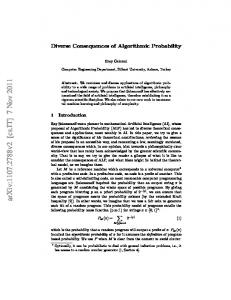
directly within some coding scheme. For example, if w is a parameter vector, its elements can be coded with some number of bits (precision) yielding the amount of information I(w). This idea gives rise to rather natural technique for specifying prior probabilities. It is unified within the Minimum Description Length principle that can verbally be formulated as [13]: the best model of the given data source is the one which minimizes the sum of – the length, in bits, of the model description; – the length, in bits, of data encoded with the use of the model. Usage of the MDL principle in pattern recognition is now widespread. For example, it was applied to choose appropriate complexity of nonlinear discrimination functions [14], support vector models [15], and the number of components in mixture models [16]. Consider the task of pattern recognition in the case of two classes, and generalized discrimination functions defined as n 1, κ(x | w ) < 0, κ(x | w ) = ∑ wi yi (x) = wY (x) , ϕ(x) =  . (4) i =1 2, κ(x | w ) > 0, where the pattern d defined as the feature vector x, the vector w is the parameter vector of the discrimination function κ(x | w ) , yi (x) is i-th generalized feature that is deterministically computed for the pattern x. In the discrimination function approach the MDL criterion has the form L({hi }in=1 , w | {xi }in=1 ) meaning that only class labels are considered as the given data to be encoded using prior information about feature values, and each model is specified by its parameter vector. Within some simplification assumptions one can obtain n M n ε 2 (w ) 2 2 , ε ( w ) = ∑ [z i − w Y ( x ) ] , (5) L({hi }in=1 , w | {xi }in=1 ) = log 2 n + log 2 2 2 n i =1 where M is the number of components in the parameter vector w, and zi=–1 if i-th vector belongs to the first class, and zi=1 if i-th vector belongs to the second class. The equation (5) can be used to select among the discrimination functions with different number of parameters. As an example, polynomial discrimination functions with different number of parameters (degrees of polynomials) were found for the set of patterns shown on the Figure 1. Patterns belong to two classes indicated using different labels (circles and crosses). Characteristics of the discrimination functions with minimum round-mean-square error ε2(w) for different number of parameters M can be found in the Table 1. It can be seen that the solution with the minimum description length has also the best recognition rate on the new patterns (%test), which is not directly corresponds to the recognition rate on the learning sample (%learn).

Figure 1. Discrimination functions with 4, 9, 16, and 25 parameters

4

Table 1. Comparison of discrimination functions of different complexity

№ 1 2 3 4

M 4 9 16 25

%learn 11.1 2.8 2.8 0.0

%test 4,3 4.0 10.1 19.4

L, bits 31.2 30.9 51.7 62.0

This is the traditional way to use the MDL principle in order to avoid overlearning that appears very fruitful in practice. At the same time, heuristic coding schemes specifying restricted subfamily of models are to be introduced for each particular task. Search within such subfamily can be easy, but only a priori restricted set of regularities can be captured. 4. Algorithmic complexity and probability The MDL principle was formulated above without explicit theoretical foundations. To be more precise, the technique for estimating I(w) on the base of the length of encoded values w within some coding scheme was not proven. The best theoretical foundation for defining information quantity without usage of probability can be found in algorithmic information theory. Consider the following notion of (prefix) algorithmic complexity of a binary string β introduced by A.N. Kolmogorov [17]: KU (β) = min[l (α) | U (α) = β] , (6) α

where U is a universal Turing machine (UTM), α is an arbitrary algorithm (program for UTM), and l(α) is its length. The expression U(α)=β means that the program α being executed on the UTM U produces the string β. In accordance with this notion, information quantity (defined as algorithmic or Kolmogorov complexity) contained in the data (string) equals to the length of the shortest program that can produce these data. In contrast to Shannon theory, this notion of information quantity relies not on probability, but on pure combinatorial assumptions. The MDL principle can be derived from the Kolmogorov complexity if one divides the program α=µδ into the algorithm itself (regular component of the model) µ and its input data (random component) δ: KU (β | µ) = min[l (δ) | U (µδ) = β] , KU (β) = min[l (µ) + KU (β | µ)] (7) δ

µ

where K(β | µ) is a specific form of the conditional complexity, which is defined for the string β relative to the given model µ. Consequently, one would like to choose the best model by minimizing the model complexity l(µ) and the model “precision” K(β | µ)=l(δ) simultaneously, where the string δ can be considered as deviations of the data β from the model µ: (8) µ* = arg min[l (µ) + KU (β | µ)] . µ

Algorithmic information theory not only clarifies the problem of the model selection criterion, but also specifies the most universal model space. Indeed, any (computable) regularity presented in the given data can be found in this model space. However, the equation (8) cannot be applied directly. The main reason is the problem of search in the Turing-complete model space. That’s why loose definitions of the MDL principle are used in practice. Another problem consists in “excessive universality” of the criterion (8). It incorporates the universal prior distribution of model lengths l(µ) or prior probabilities 2–l(µ). This distribution is independent of the specific task to be solved implying that any available information should be directly included in the string β. For example, it is impossible to use the equation (8) in order to select the best 5

class h for the single pattern d. An attempt to calculate l(h)+KU(d | h) instead of I(h)+I(d | h) will be unsuccessful, because if one takes d and h as individual data strings, there will be no mutual information in them. Available information in the pattern recognition task is the training set {di, hi}. One can try to find the best model for these data µ* = arg min[l (µ) + KU ({d i , hi } | µ)] . (8) µ

If there is a statistical connection between patterns di and their labels hi, it can be captured by µ*, because algorithmic models can also contain optimal codes for random variables. This statement of the induction task is possible (although additional prior information is difficult to include in it), but how to recognize new patterns on the base of such µ*? The simplest yet powerful idea is to explicitly consider the pattern recognition problem as the mass problem. 5. Between theoretical and practical MDL As it was pointed out, the MDL principle helps to partially solve in practice such problems as overfitting, overlearning, oversegmentation, and so on. However, it can also be seen that coding schemes for description length estimation are introduced heuristically in the MDL-based methods. Ungrounded coding schemes are non-optimal and non-adaptive (independent of the given data). These schemes define algorithmically incomplete model spaces that cause corresponding methods of pattern recognition to be fundamentally restricted. Thus, there is a large gap between the theoretical MDL principle with the universal model space and prior probability distribution and its practical applications. Tasks of inductive inference should be considered as mass problems in order to bridge this gap. Indeed, trained classifiers are usually applied independently for each pattern. In most cases the algorithmic complexity of concatenation of some data strings β1β2…βn is strictly smaller than the sum of their individual algorithmic complexities: n

KU (β1β 2 ...β n )