Pre-Runtime Scheduling for Embedded Hard Real ... - Semantic Scholar

Pre-Runtime Scheduling for Embedded Hard Real-Time Systems Using Time Petri Nets Raimundo Barreto

Paulo Maciel Meuse Oliveira J´unior Centro de Inform´atica (CIn) Universidade Federal de Pernambuco (UFPE) PO Box 7851, 50732-970, Recife-PE-Brazil {rsb, prmm, mnoj}@cin.ufpe.br

Abstract Finding a feasible schedule is not trivial, because this problem is NP-Hard in its general form. There are two general approaches for scheduling tasks in real-time systems: runtime (or on-line) and pre-runtime (or off-line) scheduling. For many cases, runtime methods do not find a feasible schedule even if such a schedule exists. Such situations often occurs when the design model imposes intertask relations, such as precedence and exclusion relations. The method proposed in this work finds a pre-runtime scheduling, when one exists, using state space exploration. The main problem with such method is the space size, which can grow exponentially. This paper shows how to minimize this problem using the proposed modeling methodology. Furthermore, the algorithm is a depth-first search method on a labeled transition system derived from the time Petri net model. Keywords: State-Space Exploration, Labeled Transition Systems, Pre-runtime scheduling, Distributed Embedded Real-Time Systems.

1 Introduction

even if such schedule exists [17]. The approach presented here uses pre-runtime scheduling, where the schedule is computed off-line. This solution is inflexible, but it reduces the runtime resources and context switching. As it is assumed safety-critical systems, the predictability is an important concern, mainly due to the use of arbitrary precedence and exclusion relations. In this paper, the task model is composed by: (i) a set of preemptable tasks with bounded discrete time values (such as period, deadline, release, and computation time); and (ii) intertask relations, such as precedence and exclusion relations. Each task ti may consist of a finite sequence of n[t ] segments t0i ,t1i , · · ·, ti i . Besides that, during the segment’s execution not any segment can preempt it. This work uses state space exploration because it presents a complete automatic strategy for verifying finitestate systems [10]. In spite of a scheduling can be found using such strategy, it may be limited due to the size of its state space. The proposed approach tackles this problem by applying a depth-first search algorithm in a reduced state space. This paper extends previous work [4] in order to tackle scheduling in distributed systems. This work is organized as follows: Section 2 summarizes the related works. Section 3 presents the computational model. Section 4 describes the formal modeling methodology, Section 5 shows how to synthesize the preruntime scheduling, and Section 6 presents experimental results. Finally, Section 7 concludes the paper.

Embedded hard real-time systems are dedicated computer applications that satisfy specific timing constraints, that is, they must guarantee that all tasks are completed before their deadlines. For meeting this requirement, scheduling performs an important role. There are two general approaches for scheduling tasks in real-time systems: run- 2 Related Work time and pre-runtime scheduling. Runtime scheduling is computed on-line as tasks arrive, using a priority-driven Xu and Parnas [17] present an algorithm that finds an opapproach. However, in many situations this approach can timal pre-runtime schedule on a single processor for realconstrain the possibility of finding a feasible schedule, time process segments with release, deadlines, and arbi-

trary exclusion and precedence relations. The optimality is given for the schedules with minimum lateness (maximum difference between the deadline and completion time of all segments). Besides the importance of this work, it was not presented real-world experimental results. Shepard and Gagn´e [14] extended the work of [17] by proposing an implicit enumeration technique for dealing with multiprocessors, but as pointed out in [1], the algorithm occasionally fails to find existing feasible schedules, since it attempts to reduce schedule lateness by modifying only the schedule of the processor running the latest task. Abdelzaher and Shin [2] proposed an extension to the Xu and Parnas’ [17] pre-run-time scheduling algorithm in order to deal with distributed real-time systems. This algorithm takes into account delays and the precedence relations imposed by interprocess communications. The proposed solution considers many possibilities for improving the scheduling lateness at the cost of complexity. The scheduler synthesis proposed by Altisen et.al. [3] uses an extension of Petri nets called PND (Petri Nets with Deadline) as modeling language and TAD (Timed Automata with Deadlines) as semantic model. Their approach synthesizes all dynamic on-line schedulers satisfying a given property. Our work does not generate on-line scheduling but, instead, off-line scheduling because of predictability issues. In addition, our work uses elementary net structures for deal with deadline checking, not requiring any extensions. Several authors also use Petri nets in scheduling theory. Even so, they are concerned with schedulability analysis, e.g. [15], which rely on a well-known fixed-priority policy. Fixed priority policies may not find feasible schedules if arbitrary precedence and exclusion relations are considered. Bruno et. al. [5] present a schedulability analysis, using high-level Petri nets, based on PROTOB formalism (an object-oriented methodology). But, this work does not generate the feasible schedules, but it relies on Xu and Parnas’ algorithm [17] in order to find them. Comparing our approach with [2] and [16], it differs in the sense that: (1) In order to search for a feasible scheduling, these works model the scheduling problem, not the system. We use a time Petri net formalism for system’s modeling, where this model is used for finding a feasible scheduling using a multiprocessor architecture. However, the model can also be used to synthesize predictable and timely scheduled code. This is an ongoing project we are researching; (2) The use of Petri net analysis techniques allows one to check several system properties, such as, feasible firing schedules, state reachability, deadlock-freedom, starvation-freedom, boundedness, fairness and so on; and

(3) The proposed approach considers heterogeneous processors, preemptive tasks, and takes into account the cost for intertask communications. The main disadvantage of the approach proposed is that allocation of tasks to processors has to be made in advance by the designer. However, it is not a great limitation since there are several works that deal with this class of problem. Nevertheless, at the best of our present knowledge, there is no similar work modeling hard real-time systems (using formal methods) for pre-runtime scheduling considering the elements described above.

3 Computational Model The computational model syntax is given by a time Petri net [11], which is a Petri net [13] extended with time, and its semantic uses a labeled transition system. A time Petri net is a bipartite directed graph represented by a tuple TPN = (P, T, F, W, m0 , I). P (ordered set of places) and T (ordered set of transitions) are non-empty disjoint sets and represent the two types of nodes in the graph. The edges are represented by F ⊆ (P × T )∪(T × P ), which is a flow relation. W : F → N represents the weight of the flow relation F . m0 : P → N is the initial marking. Finally, I is a mapping called static firing interval I : T → N × N. A set of enabled transitions is denoted by: ET (mi ) = {t ∈ T | mi (pj ) ≥ W (pj , t)}, ∀pj ∈ P. Implying that transition t ∈ ET (mi ) can fire leading to a new marking. The timing constraints are represented by the static firing interval I(t) for each transition t, where I(t)=(EFT(t), LFT(t)) ∀t ∈ T . This bounds are called earliest and latest firing time, respectively. Each enabled transition has an implicit clock C(t), defined by C : ET (m) → N, where it is a clock mapping (or vector), which represents the time elapsed since the respective transition enabling. The firing semantics is single server semantic with restart, i.e., the firing strategy is to fire single transitions implying that no transition may be fired more than once simultaneously, and its clock is reset to zero after the firing. As time elapses and an enabled transition t does not fire, this is represented by its dynamic firing interval ID (t) = (DEF T (t), DLF T (t)), ∀t ∈ ET (m). ID is computed as follows: DEF T (t) = max (0, EF T (t) − C(t)), and DLF T (t) = LF T (t) − C(t)). In other words, the dynamic firing interval for an enabled transition t is calculated by its static firing interval decremented by its current clock value. The lower bound is truncated, when necessary, to nonnegative values.

Definition 3.1 (States) Let T P N be a time Petri net, and C be the respective clock mapping. S ⊆ M × C is the set of states of the T P N , defined by a pair (m, C), where m corresponds to a reachable marking of a TPN, and C is its respective vector of clock values.

This definition states that the firing of a transition ti , at a specific time θi in previous state (si−1 ) defines the next state (si ). The modeling methodology, as it will be presented later, guarantees that the desirable final marking M F is unique, well-known, and has the property that it always leads to a dead state.

F T (s) is the set of firable transitions at state s defined by: F T (s) = {ti ∈ ET (m)|DEF T (ti ) ≤ min (DLF T (tk ))}, ∀tk ∈ ET (m). This definition also 4 Modeling Real-Time Systems implicitly defines the firing interval (or firing domain) for ti at a specific state s, which is defined as: F I(ti ) = Petri nets allows one to model several kinds of model[DEF T (ti ), min (DLF T (tk )), ∀tk ∈ ET (M ). ing situations present in most concurrent systems, such as precedence and exclusion relations, data-dependencies, Definition 3.2 (Labeled Transition System) A labeled computations, communication protocols, multiprocessing, transition system is a quadruple L= (S, Σ, →, s0 ), where synchronization mechanisms, shared resources, and so on. S is a finite set of discrete states, Σ is an alphabet of labels The proposed modeling method allows one to represent representing activities, → is the transition relation, and s0 heterogeneous multiprocessor systems. Nevertheless, in is the initial state. this work, only homogeneous processors and designer The semantic of a time Petri net P = made allocation are considered. (P, T, F, W, M0 , I) is defined by associating a labeled transition system LP = (S, Σ, →, s0 ) such that: 4.1 Problem Transformation (i) S is the set of states of P; (ii) Σ ⊆ (T × N) is a set of activities labeled with (t, θ) corresponding to the Let T be a set of n tasks T = { T 1 , T 2 , . . ., T n }, where firing of a firable transition at a specific time value in the each T i is characterized by a tuple (Ri , Ci , Di , Pi ), where firing interval F I(s), ∀s ∈ S; (iii) → ⊆ S × Σ × S; Ci ≤ Di ≤ Pi , Ri is its release time, Ci the computation (iv)s0 = (m0 , c0 ), where m0 is the initial marking of P, time, Di the deadline, and Pi the period. and c0 (t) = 0 ∀t ∈ ET (m0 ). In pre-runtime scheduling, it is only possible to schedule periodic tasks. However, it is possible to transDefinition 3.3 (Reachable States) Let LP be a LTS delate a sporadic task into an equivalent periodic one [12]. rived from a time Petri net P, and si = (mi , ci ) a reachable One technique for achieving this is to translate each spostate. sj =fire(si , (t, θ)) denotes that firing a transition radic task (C , D , M IN ) into a corresponding periodic s s s t at time θ from the state si , a new state sj = (mj , cj ) is task (Rp , Cp , Dp , Pp ), satisfying the following conditions: reached, such that: Cp = Cs , Ds ≥ Dp ≥ Cs , Pp ≤ min(Ds − Dp + 1, M INs ). For example, suppose the sporadic task is de• ∀p ∈ P, mj (p) = mi (p) − W (p, t) + W (t, p) fined by (2, 9, 10). The corresponding periodic process • ∀tk ∈ ET(mj ) can be: (0, 2, 2, 8), because the conditions are satisfied. if (tk = t)  0, For more information the reader is referred to [12]. Even 0, if (tk ∈ ET (mj ) − ET (mi )) cj (tk ) = though sporadic tasks arrive randomly, information about  ci (tk ) + θ, else sporadic events can be buffered until it can be handled by The aim of this paper is to find a firing schedule that sat- periodic tasks. The pre-runtime approach consists of computing a isfies all specified constraints. The definition of a feasible schedule off-line for the entire set of periodic tasks occurfiring schedule is as follows. ring within a time period that is equal to the least common Definition 3.4 (Feasible Firing Schedule) A firing multiple (LCM) of the periods of the given task set. The schedule is feasible, starting from state s0 , iff LP has a LCM is also called schedule period (P ). Any feasible S (t1 ,θ1 ) (t2 ,θ2 ) (tn ,θn ) direct path: s0 −→ s1 −→ s2 − − → sn−1 −→ sn schedule obtained for that new period is also feasible for where si =fire(si−1 , (ti , θi )) i > 0, ti is a firable any longer time, since the schedule can be indefinitely retransition at state si−1 , θi is the firing time, and the peated. Within the schedule period (PS ), there are several marking of the final state sn corresponds to the desirable tasks’ instances of the same task, where N (T i ) = PS /Pi final marking (M F ). gives the number of instances for T i . Table 1 presents a

since the timing interval for the computation transition is equal to the task computation time, that is [C,C];

Table 1: Specification of tasks task R C D P T1 0 2 7 8 T2 2 3 6 6

b) all-preemptive, where the task is implicitly split into all possible segments1, that is, the computation is performed one unit at each time. This model allows another conflicting task to run, in this case, implying in preemption. Note the difference between the timing interval for the transition computation and weight of arcs between Figure 1(a) and (b);

Pproc

(a)

P1

P2

...

P3 computation [C,C]

proc-grant

release

end

Pproc

(b)

C

P1

P3

P2 proc-grant

release

computation [1,1]

c) defined segments, where the task is split into two segments explicitly defined.

C

... end tmd2 [0,0]

tph2 [0,0]

Pproc

P20

P24

P22 3

release

P2 proc-grant-s1

P3 comp.seg1 [cs1,cs1]

proc-grant-s2

...

P5

P4 comp.seg2 [cs2,cs2]

end

P27

P26 tc2 [3,3]

tp2 [0,0]

tr2 [2,2]

ta2 [6,6]

Pstart

4

Pproc

P1

P25

P23

P21

(c)

tstart [0,0]

tend [0,0] Pend

3 ta1 [8,8]

Figure 1: Modeling Scheduling Methods

P11

tp1 [0,0]

tr1 [0,0] P13

tc1 [2,2]

P15

P16

P17

2 P10

P14

P12 tph1 [0,0]

task model containing two tasks: T 1 and T 2 . For this example, seven tasks’ instances have to be scheduled, since Figure 2: PN Model for Table 1 PS = 24, N (T 1 ) = 3, and N (T 2 ) = 4. Each timing constraints of task instances have to be transformed to consider Figure 2 presents a non-preemptive time Petri net model this new schedule period. Table 2 depicts the modified timfor the case study shown in Table 1. As it can be seen, ing constraints. it does not model explicitly all seven tasks’ instances. Instead, it makes an optimization in the sense that it models Table 2: Task set modified the two original tasks and the period of time when all inT 01 T 11 T 21 T 02 T 12 T 22 T 32 stances of a task need to be executed. R 0 8 16 2 8 14 20 Processor C 2 2 2 3 3 3 3 Pproc D 7 15 23 6 12 18 24 P 24 24 24 24 24 24 24 task structure tmd1 [0,0]

ta

tr

P5

P3

P1

tp

P6

tc

Pout

N(T)-1

4.2 Translating Task Model to TPNs

Pin

P4

P2 tci

arrival

tmd

deadline

In this approach, the definition of tasks’ segments also defines the preemption points, because when a segment Figure 3: Building blocks for a complete task is running, it cannot be preempted. Considering that the task computation time is equal to C time units, where Figure 3 is used to show the three main building blocks C = cs1 + cs2 , Figure 1 presents three ways for modeling for modeling a real-time task. These blocks are: scheduling methods: a) all-non-preemptive, where the processor is just released when the computation is entirely finished,

1 One

task time unit is the smallest indivisible granule of a task. If the task computation time is equal to C time units, then the task can be split into at most C segments.

a) Task Arrival. The block Arrival models the periodic invocation for all task’s instances in the schedule period (PS ). A transition tph (in a task model) models the phase shifting arrival of the first instances of a task. For instance, two tasks, A and B, have the equal timing constraints (RA , CA , DA , PA ) = (RB , CB , DB , PB ) = (0, 5, 5, 10). This system is not schedulable. However, if a phase shift is specified, i.e. tphB = [5, 5], the system becomes schedulable. Similarly, transition ta models the periodic arrival (after the phase shifting) for the remaining instances. Note the weight of the arc between tph and P1 , which models the invocation of all remaining instances. b) Deadline Checking. In the block Deadline the transition tmd models deadline missing. However, some works (e.g. [3]) extended the Petri net to deal with deadline checking. This methodology uses elementary net structures to capture deadline missing. The scheduling algorithm eliminates states that leads to deadline missing. c) Task Structure. The building block Task Structure (Fig. 3) models: release time, processor granting, computation, and processor releasing. The task’s computation can be modeled by a finite number of sequential transitions, where each transition corresponds to a task’s segment [17], during which any other segment cannot preempt it. trelease

tgrant-proc

B tsequence

tgrant-proc

...

tcomp

tgrant-proc

texcl

trelease

CA

tfinal CA

...

Pexclusive

Pproc

Task B

...

trelease

...

CB

CB tgrant-proc

tcomp

tfinal

Figure 5: Modeling (A EXCLUDES B) relation the A EXCLUDES B exclusion relation using a preemptive scheduling method.

5 Off-line Scheduling Synthesis This section investigates how to find a feasible pre-runtime schedule using state space exploration. First of all, it describes how to minimize the state space size, and next, it presents an algorithm that implements the proposed method.

5.1 Minimizing State Space Size Limiting Interleaving by Modeling.

tcomp

A

trelease

Task A

tcomp

The state space increases because of the interleaving of activities. For instance, the analysis of n concurrent activities has to search all n! interleaving possibilities of these activities. When explicitly modeling the dependencies between activities certainly the state space decreases.

Figure 4: Modeling (A PRECEDES B) relation Now, considering intertasks relations, it has: a) Precedence Relations. A task (or segment) ti is said to precede another task (or segment) tj , if tj can only start execution after ti has finished. In general, this kind of relation is suitable when a task (successor) needs information that is produced by another task (predecessor). This relation impose equal period for the two tasks. Precedence relation can be modeled as shown in Figure 4. b) Exclusion Relations. A task (or segment) ti is said to exclude another task (or segment) tj , if no execution of tj can occur while task ti is executing. In other words, the task ti could not be preempted by task tj . Exclusion relations may prevent simultaneous access to shared resources. It is worth noting that, the exclusion relation is not symmetrical, that is, when A EXCLUDES B it does not necessarily implies that B EXCLUDES A. Figure 5 models

Partial-Order Reduction. Several techniques have been developed to tackle the state explosion problem, among them, reduction techniques that exploit the independence of events. If activities can be executed in any order, such that the system always reaches the same state, these activities are independent. In other words, it does not matter in which order the activities are executed. Methods based on the independence of activities are called partial-order reduction methods [10]. It is guaranteed by the modeling methodology and the proper definition of firable transition set that, all activities (or transitions in the context of Petri nets) where the pre-conditions are satisfied have to be executed. The independent activities are those that do not disable any other activity, such as: arrival, release, precedence, computation, processor releasing, and end-task. What this reduction method proposes is

to give to each class of independent activities a kind of priority. The other activities, the dependent ones, like exclusion and processor granting, will have the same and lowest priority. Therefore, when changing from one state to another state, it is sufficient to analyze the class with higher priority and simply to prune the other ones. When all independent activities are executed, certainly the final state is the same, because the order between them does not matter. This reduction is important due to two reasons: (i) depleting the amount of storage; and (ii) finding the negative result, when the system does not have a feasible schedule, rapidly. Removing Undesirable States. In Section 4 it is presented how to model undesirable error markings, for instance, markings that represent missed deadlines. The method proposed is of interest in schedules that do not reach any of these undesirable markings. For this reason, when generating the LTS, the transitions that lead to undesirable error states, denoted by T E , may be discarded.

5.2 Scheduling Algorithm

Table 3: Illustrative Example #

st

ET

C

FT

trans

1 2 3 4 5 6 7 8 9 10 11 12 13 14 15 16 17 18 19 20 21 22 23 24 25 26 27 28 29 30 31 32 33 34 35

0 1 2 3 4 5 6 7 8 9 10 11 12 13 14 15 16 17 13 14 15 16 17 18 19 20 21 22 23 24 25 26 27 28 29

{tstart} {tph1,tph2} {tph2,tr1,ta1,td1} {tr1,ta1,ta2,td1,td2} {tp1,ta1,ta2,td1,td2} {tr2,tc1,ta1,ta2,td1,td2} {tc1,ta1,ta2,td1,td2} {tp2,ta1,ta2,td2} {tc2,ta1,ta2,td2} {ta1,ta2} {ta1,ta2,tr2,td2,} {ta1,ta2,tr1,tr2,td1,td2} {ta1,ta2,tr2,td1,td2,tp1} {ta1,ta2,td1,td2,tp1,tp2} {ta1,ta2,td1,td2,tc1} {ta1,ta2,td2,tp2} {ta1,ta2,td2,tc2} {ta1,ta2,td2,tr2} {ta1,ta2,td1,td2,tp1,tp2} {ta1,ta2,td1,td2,tc2} {ta1,ta2,td1,tp1} {ta1,ta2,td1,tc1} {ta1,ta2,td1,tc1,tr2} {ta1,ta2,tr2} {ta1,ta2,tp2} {ta1,ta2,tc2} {ta1,ta2} {ta2,td1,tr1} {ta2,td1,tp1} {ta2,td1,tc1} {td1,tc1,td2,tr2} {td2,tr2} {td2,tp2} {td2,tc2} {tend}

{0} {0,0} {0,0,0,0} {0,0,0,0,0} {0,0,0,0,0} {0,0,0,0,0,0} {2,2,2,2,2} {0,2,2,2} {0,2,2,2} {5,5} {6,0,0,0} {0,2,0,2,0,2} {0,2,2,0,2,0} {0,2,0,2,0,0} {0,2,0,2,0} {2,4,4,0} {2,4,4,0} {4,0,6,2} {0,2,0,2,0,0} {0,2,0,2,0} {3,5,3,0} {3,5,3,0} {4,0,4,1,0} {4,1,1} {5,2,0} {5,2,0} {8,5} {5,0,0} {5,0,0} {5,0,0} {1,1,0,0} {1,1} {2,0} {2,0} {0}

{tstart} {tph1,tph2} {tph2,tr1} {tr1} {tp1} {tr2,tc1} {tc1} {tp2} {tc2} {ta2} {ta1,tr2} {tr1,tr2} {tr2,tp1} {tp1,tp2} {tc1} {tp2} {ta2,td2} {td2} {tp1,tp2} {tc2} {tp1} {ta2} {tc1} {tr2} {tp2} {tc2} {ta1} {tr1} {tp1} {ta2} {tc1} {tr2} {tp2} {tc2} {tend}

{tstart,0} {tph1,0} {tph2,0} {tr1,0} {tp1,0} {tr2,2} {tc1,0} {tp2,0} {tc2,3} {ta2,1} {ta1,2} {tr1,0} {tr2,0} {tp1,0} {tc1,2} {tp2,0} {ta2,2} {td2,0} {tp2,0} {tc2,3} {tp1,0} {ta2,1} {tc1,1} {tr2,1} {tp2,0} {tc2,3} {ta1,0} {tr1,0} {tp1,0} {ta2,1} {tc1,1} {tr2,1} {tp2,0} {tc2,3} {tend,0}

be bound, and (ii) the timing constraints are by definition bounded and discrete, this implies that the LTS is finite and thus the proposed algorithm always finishes. This algorithm combines two features: partial LTS generation and scheduling search. The only way the algorithm returns TRUE is when it has reached a desired final marking (M F ), implying that a feasible schedule was found (line 3). The state space generation algorithm is modified (line 4) to incorporate the pruning from the partial-order reduction technique, and removing transitions (T E ) that lead to undesirable states. The function fire (line 7) returns a Algorithm 5.1 (Scheduling Synthesis) new generated state (S ′ ) due to the firing of transition tk 1 schedule-synthesis(S) at time θ (following Def. 3.3). When returning with suc2 { 3 if (S.M = MF ) return TRUE; cess from a recursive call, the algorithm generates a transi4 PT = remove-undesire(partial-order(firable(S))); tion system, which represents the found feasible schedule 5 if (|PT| = 0) return FALSE; through the function add-in-trans-system (line 9). 6 for each (ht, θi ∈ PT) { 7 S’= fire(S, t, θ); In case the system does not have a feasible schedule, 8 if (schedule-synthesis(S’)) { 9 add-in-trans-system (S’,S,t,θ); the proposed method searches the whole reduced state 10 return TRUE; space. Starting from the transition systems generated by 11 } 12 } our framework, it is not complicated to translate into a tim13 return FALSE; ing diagram. The actual implementation of the pre-runtime 14 } scheduler can be reduced to an executive cyclic using a lookup table. The Algorithm 5.1 describes the proposed solution. As Table 3 shows the dynamics of the Algorithm 5.1 applied it can be seen, it is very simple and easy to understand. to the TPN model in Figure 2. In this table we see, for each Considering that, (i) the Petri net model is guaranteed to reachable state, the enabled transition set, the respective The algorithm proposed in this work is a depth-first search method on a LTS. Therefore, the LTS is not completely generated before the search, but it is generated partially, as needed. The LTS is reduced since not all transitions are evaluated due to the partial-order reduction method and the undesirable transitions (which certainly lead to undesirable states). The stop criterion is when the desirable final marking M F is reached, which represents that a feasible firing schedule (Def. 3.4) was found.

6 Experimental Results Table 4 shows a summary of the experimental results. In the table, U represents the processor utilization degree, and state-min represents the minimum number of states to be verified, which is equal to the number of transitions in the PN model. The time is expressed in milliseconds. The results presented were obtained for finding the first feasible schedule. All experiments were performed on a dual Pentium-III 600 Mhz processors with 768 MB RAM, OS Linux, and compiler GCC 2.95.4. Xu-Parnas Example 3. This example case study is the third presented in [17] that shows that schedules having intertask relations (such as precedence and exclusion) cannot be solved through static/dynamic priority-driven scheduling algorithms (for instance, earliest deadline first, or deadline monotonic). The timing constraints (release, computation, and deadline, respectively) are: A = (0, 30, 80); B = (20, 20, 81); and C = (40, 30, 70). The exclusion relation is: B EXCLUDES C. The TPN model considers a preemptive (P) scheduling method. In this case, the tasks are split into all possible segments, that is, eighty (30+20+30) segments. The approach searched 1566 states, where the minimum number of states is 171 states, and found a feasible schedule in 790 ms using a preemptive scheduling method. The time spent for finding a feasible schedule could be reduced if the model does not impose several segments. Simple Control Application. This case study is a simple control application described originally in [8]. The

S12

M24

M17

S6

S7

S18

M27

S16

S9

S8

S26 S28

P3

S5

S4

S25

M15 S11 S10

S22

S20

S19

S2 P2

M21

M13

S1

S14

P1

S3

clock values, the firable transition set, and the chosen transition to be fired at a specific time instant. At line 14, two transitions (tp1 and tp2 ) are firable. As it can be seen, the decision taken in a state, may change the firable sequences. In this specific situation, the possible execution of task T1 on the processor (tp1 ) is a wrong choice because, after that, task T2 misses its deadline (line 18). The algorithm backtracks to state 13 (line 19) and tries another alternative, now granting the processor to the task T2 (tp2 ). This new decision leads to a feasible schedule, since in the line 35 the firing of transition tend reaches the desired final marking.

S23

P4

Table 4: Experimental results summary Example inst. state-min found time meth Xu 4 171 1566 790 P Control 28 50 50 4.4 DS Mine Pump 782 3130 3268 105 NP

Figure 6: The Simple Control Application Graph

Table 5: Task Model for the Simple Control Application Segment Ci Di Segment Ci Di S1 3 100 M15 1 S2 3 200 S16 10 100 S3 3 40 M17 1 S4 3 100 S18 1 100 S5 3 100 S19 5 200 S6 3 200 S20 7 100 S7 2 100 M21 1 S8 2 100 S22 6 40 S9 2 100 S23 10 200 S10 2 40 M24 1 S11 2 200 S25 2 100 S12 2 200 S26 1 100 M13 1 M27 1 S14 15 100 S28 7 100

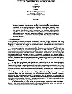
system consists of a sensory device mounted on a motorized platform that must detect and track specific objects in the environment. Four processors connected by a single bus control the system. The model consists of 6 tasks split into 22 segments, which exchanges 10 messages, 6 of them are sent across processor boundaries. Figure 6 shows the computational graph for this application, presenting the segments allocated to processors, and its communication pattern. Table 5 gives the computation time and deadline for each segment as well as the transmission time for each interprocessor message. The scheduling is found with no overhead, since the proposed algorithm only examined the minimum number of states (in this case 50) in 4.4 ms using defined segment scheduling method.

Mine Drainage System. This example is another realworld application, namely the mine pump controller. Detailed specification for this example can be found in [6, 7]. This problem has not tight timing constraints in general, but the schedule for this problem is interesting because it has 10 tasks, implying 782 tasks’ instances and, at the beginning, all 10 tasks arrive at the same time. Our solution searched 3268 states (where minimum number of states is 3130), in this case having an overhead of 138 states (4.4%), which is very low considering the complexity of this example. The time performance is 105 ms, and it used a nonpreemptive (NP) method.

[3]

[4]

[5]

7 Conclusions This paper proposed a formal modeling methodology based on time Petri nets, and a framework for pre-runtime scheduling synthesis using a reduced state space exploration algorithm. The real-time task specification can be very general, since it can have resource and timing constraints, and intertask relations, such as precedence and exclusion relations. The algorithm is a depth-first search method on a finite LTS derived from a TPN model. When searching for a feasible schedule, the algorithm suffers from the state space explosion problem. In order to maintain the state space growth under control, the proposed method uses minimization techniques. Considering the experimental results, feasible schedules were found after analyzing a reduced number of states. The algorithm presented always finds a schedule provided that one exists. The proposed modeling and the scheduling synthesis are an important step toward embedded real-time software synthesis tools. Thus, it is planned to generate complete executable code from the formal model. This can be solved through TPN with tasks, which is an extension of TPN, which annotates transitions with program code. Currently, we are also working on a tool for translating real-time specifications into Petri net models. Another extension of this research is to consider the addition of some flexibility into the pre-runtime scheduling [9].

References [1] T. F. Abdelzaher and K. G. Shin. Comments on a pre-runtime scheduling algorithm for hard real-time systems. IEEE Trans. Soft. Engineering, 23(9):599–600, September 1997. [2] T. F. Abdelzaher and K. G. Shin. Combined task and message scheduling in distributed real-time systems. IEEE

[6]

[7]

[8]

[9]

[10]

[11]

[12]

[13] [14]

[15]

[16]

[17]

Trans. Parallel and Distributed Systems, 10(11):1179– 1191, November 1999. K. Altisen, G. G¨obler, A. Pnueli, J. Sifakis, S. Tripakis, and S. Yovine. A framework for scheduler synthesis. IEEE Real-Time System Symposium, pages 154–163, Dec. 1999. R. Barreto, S. Cavalcante, and P. Maciel. A time petri net approach for finding pre-runtime schedules in embedded real-time systems. In 1st Int. Workshop on Embedded Computing Systems (ECS’04) in conjunction with the 24th Int.Conf. on Distributed Computing Systems (ICDCS’04). IEEE CS Press, march 2004. G. Bruno, A. Castella, G. Macario, and M. Pescarmona. Scheduling hard real time systems using high-level petri nets. In Jensen, K., editor, Lecture Notes in Computer Science; 13th International Conference on Application and Theory of Petri Nets 1992, Sheffield, UK, volume 616, pages 93–112. Springer-Verlag, June 1992. A. Burns and A. Wellings. HRT-HOOD: A structured design method for hard real-time systems. Real-Time Systems Journal, 6(1):73–114, 1994. S. Cavalcante. A Hardware-Software Co-design System for Embedded Real-Time Applications. PhD Thesis, University of Newcastle Upon Tyne, June 1997. M. DiNatale and J. A. Stankovic. Dynamic end-to-end guarantees in distributed realtime systems. In IEEE RealTime Systems Symposium, pages 216–227, 1994. G. Fohler. Flexibility in Statically Scheduled Hard RealTime Systems. PhD thesis, Technische Universit¨at Wien, Institut f¨ur Technische Informatik, Vienna, Austria, 1994. P. Godefroid. Partial Order Methods for the Verification of Concurrent Systems: An Approach to the State-Explosion Problem. PhD Thesis, University of Liege, Nov. 1994. P. Merlin and D. J. Faber. Recoverability of communication protocols: Implicatons of a theoretical study. IEEE Transactions on Communications, 24(9):1036–1043, Sept. 1976. A. K. Mok. Fundamental Design Problems of Distributed Systems for the Hard-Real-Time Environment. PhD Thesis, Dept Electrical Engineering and Computer Science, Massachusetts Institute of Technology, May 1983. T. Murata. Petri nets: Properties, analysis and applications. Proc. IEEE, 77(4):541–580, April 1989. T. Shepard and J. A. Gagn´e. A pre-run-time scheduling algorithm for hard real-time systems. IEEE Trans. Soft. Engineering, 17(7):669–677, July 1991. D. Xu, X. He, and Y. Deng. Compositional schedulability analysis of real-time systems using time petri nets. IEEE Trans. Soft. Engineering, 28(10):984–996, October 2002. J. Xu. Multiprocessor scheduling of processes with release times, deadlines, precedence, and exclusion relations. IEEE Trans. Soft. Engineering, 19(2):139–154, February 1993. J. Xu and D. Parnas. Scheduling processes with release times, deadlines, precedence, and exclusion relations. IEEE Trans. Soft. Engineering, 16(3):360–369, March 1990.