PRECIPITATION CHANGE: MODEL SIMULATIONS AND PALEORECONSTRUCTIONS M. V. SHABALOVA1 , G. P. KÖNNEN1 and I. I. BORZENKOVA2 1 Royal Netherlands Meteorological Institute (KNMI), The Netherlands
E-mail:
[email protected] or
[email protected] 2 State Hydrological Institute, Russia E-mail:
[email protected]
Abstract. Zonal-scale patterns of precipitation change, as reconstructed for the Mid-Pliocene and the two Pleistocene optima, are compared with those generated in standard 2 × CO2 –1 × CO2 equilibrium experiments by two high-resolution GCMs of equal sensitivities of global precipitation and temperature to CO2 doubling. We find that the three warm paleoclimates, despite differences in boundary conditions/forcings, exhibit a similarity in zonal-scale patterns of change for precipitation over land in the Northern Hemisphere (NH); the between-epoch pattern correlation is 0.9 on the average. The two models give marked differences in zonal distribution of precipitation anomalies at mid-latitudes; the between-model pattern correlation for changes of precipitation over NH land is 0.4. The response of precipitation over the NH land area to the NH warming is about 10%/◦ C in the paleodata compared to 3%/◦ C in the models. The largest model/paleodata descrepancy refers to the present-day desert belt, where a large precipitation anomaly persists in all epochs. North of 50 N, the absolute values of the zonally-averaged precipitation anomalies simulated by both models fall in the range implied by the three warm paleoclimates, but they are systematically lower than the anomalies of the Mid-Pliocene. If our reconsructions are valid and if climate changes in the Mid-Pliocene were driven solely by CO2 changes, then our results suggest that models are underestimating the magnitude of the precipitation response, especially in the regions of subtropical deserts; the magnitude of the simulated temperature response at high latitudes is also underestimated. At least part of the reported model/paleodata discordance appears to be due to lack of interactive land surface package in the models examined.
1. Introduction Evaluation of climate models against empirical data is a subject of increasing relevance (IPCC, 1996). The continuous efforts to calibrate the models’ statistics in the control climate experiments with observations represent a necessary (but not sufficient) condition in the evaluation of the models’ predictive skill. The simulations of the control climate show shortcomings that are primarily attributed to flaws in the parameterizations of clouds and in the representation of sub-grid surface processes (e.g., Cess et al., 1990; Boer et al., 1992; Lau et al., 1996). A model/data inconsistency in patterns of natural low-frequency variability has also been reported (Barnett et al., 1996; Kim et al., 1996). However, even if the models were perfect in simulating the current climate, it would not be a guarantee of Climatic Change 42: 693–712, 1999. © 1999 Kluwer Academic Publishers. Printed in the Netherlands.
694
M. V. SHABALOVA ET AL.
their predictive power, because model’s parameterizations are tuned to the current climate and the sensitivity of a model may be incorrect. A next logical testing step is therefore to investigate the model’s performance in reproducing past equilibrium climates. This raises the issue of the reliability of the paleoreconstructions, given the methodological problems in the climate signal estimation from proxy data, the spatial inhomogeneity of the original data distribution and the dating problems (Crowly and North, 1991; Velichko, 1985). Although these sources of errors imply significant uncertainty in the reconstructed values at a given site, it is believed that large-scale patterns of the reconstructed temperature fields are realistically resolved (Crowley, 1993). There is an ongoing international effort to reproduce large climate changes with a number of GCMs (e.g., COHMAP, 1988; Kutzbach et al., 1993; 1996; Paleoclimate Modelling Intercomparison Project: Joussaume and Taylor, 1995). In the framework of such projects, a set of altered boundary conditions is extracted from reconstructions based on geological data from a particular paleoclimate (e.g., CLIMAP, 1976). This set is used to simulate a paleoclimate after which the simulation is compared with paleodata. A problem with this type of model/data comparison is that often the simulation has to be verified with a paleoreconstruction that is based partly on the same paleo evidence that was used to determine the boundary conditions. Therefore, a circular reasoning may be involved. A second methodological problem, which complicates the interpretation of these comparisons, is that the model sensitivity to the change of each individual boundary condition is not always known and may vary from model to model. An alternate test of the model’s predictive capacity is checking the model response to the change of one boundary condition at a time. An example is the examination of the sensitivity of simulated climates to doubling of the atmospheric CO2 concentration. The possibilities for a direct evaluation of simulated fields from sensitivity experiments against paleodata are limited as the actual realization of a past climate is generally the result of a mix of different forcings. It has been shown however (Budyko, 1988; Hoffert and Covey, 1992; Shabalova and Können, 1995), that despite the differences in forcings/boundary conditions, the response of zonally-averaged temperatures to global/hemispheric warming or even cooling is approximately the same in a number of past climate realisations. This sensitivity pattern, with quite steep amplification of temperature changes from tropics to high latitudes, is also apparent from an independent analysis of the SPECMAP timeseries (Shabalova and Können, 1995a). Under the assumption that the paleoreconstructions are valid, these results suggest that the large-scale zonal pattern of temperature changes is rather insensitive to the actual nature of the forcing, being strongly determined by internal feedback mechanisms which are universal for any climate (e.g., the positive albedo/temperature feedback at high latitudes and the negative evaporation/temperature feedback in tropics, where the evaporative cooling is shown to offset the positive water vapor/temperature feedback – see Hartmann and Michelsen, 1993). According to IPCC (1990), in a number of
PRECIPITATION CHANGE: MODEL SIMULATIONS AND PALEORECONSTRUCTIONS
695
model simulations of equilibrium climate with doubled CO2 concentration this paleopattern is indeed reproduced, at least in winter. Validating the models with respect to precipitation is a more difficult task because of two reasons. First, the paleoreconstructions of precipitation are scarce and less reliable than the temperature reconstructions, and second, the model simulations of precipitation are less solid (Stuart and Isaac, 1994; Hurrell, 1995). In spite of these limitations, the problem deserves to be addressed. The last three warm epochs – Mid-Holocene, Eemian and Mid-Pliocene – are covered by the extensive precipitation reconstructions by Borzenkova (1992) and represent therefore a potential for calibration of climate models. It should be noted that the forcing mechanisms providing for the ultimate changes in these three paleoclimates are different. In the two Pleistocene optima the changes are believed to be mainly driven by variations of the orbital and insolation parameters (e.g., Bradley, 1986). In the Pliocene however the CO2 concentration was altered. Although recent estimates yield a Mid-Pliocene CO2 level of about 30% above the pre-industrial value (Raymo et al., 1996; Crowley, 1996), compared to earlier estimates of 100% (Budyko et al., 1985; Crowley, 1991), the Mid-Pliocene climate may still be potentially used as a direct source for evaluating the equilibrium 2 × CO2 models, provided that other forcings are of minor importance. The validity of this approach relies on model experiments showing that the patterns of temperature and precipitation changes are similar for different levels of CO2 concentration, while the magnitude of changes depends on CO2 (Syktus et al., 1997). Adopting a 30% CO2 increase for the Mid-Pliocene and assuming log-linear dependence of magnitude of temperature/precipitation change on the forcing in the models (Syktus et al., 1997), the model anomalies from the 2 × CO2 equilibrium experiments should be rescaled with a factor ∼0.38 (ln(1.3)/ln(2)) to be directly comparable with Mid-Pliocene. It still remains to be seen to what extend model calibration with respect to precipitation requires a reconstruction of a paleoclimate that has been actually forced by CO2 . In any climate the hydrological cycle is closely related to the thermal regime rather than to the forcing itself. The existence of a large-scale universal pattern of temperature change in the Mid-Holocene, Eemian and Mid-Pliocene (e.g., Shabalova and Können, 1995) suggests that the calibration may be extended to the two Pleistocene periods, too, at least as far as the response of precipitation to global warming (rather than to CO2 forcing) is concerned. This type of comparison makes the scope of this paper, but because of its potential as an approximate CO2 analog, some emphasis is put on the Mid-Pliocene climate. We assume in this paper that our reconstructions are valid, or at least certain bold features in them. However, the discussions are still ongoing (e.g., Covey, 1995), and it is clear that, even with best efforts, questions will always remain about the ultimate validity of anyone’s paleoclimate reconstruction in general and about the degree of independence of precipitation and temperature reconstruction from the same proxy data in particular. On the other hand, paleodata are the only
696
M. V. SHABALOVA ET AL.
source for validating the model’s predictive skill. In this perspective, our results should be considered as a first but perhaps indicative step in attempts to evaluate the sensitivity of simulated precipitation to warming against paleodata. The outline of the paper is as follows. In Section 2 we extensively discuss the paleodata used and briefly describe the model data. In Section 3 the zonal patterns of temperature change of the two selected models in 2 × CO2 equilibrium experiments and in the two independent reconstructions of the Mid-Pliocene climate are compared. The zonal patterns of precipitation change in the two model simulations and in the three paleoclimates are described in Section 4. A model/paleo comparison is presented in Section 5. Section 6 gives a summary and conclusions.
2. Data 2.1.
PALEODATA
We used the paleoreconstructions of near-surface temperature and precipitation anomalies in the Mid-Holocene, Eemian and Mid-Pliocene by Borzenkova (1992) (hereafter referred to as reconstructions B) and additionally the reconstruction of the sea surface temperature (SST) in the Pliocene by Dowsett et al. (1996) (hereafter reconstruction D). Reconstruction D provides the Pliocene SST for February and August over an 8◦ × 10◦ spatial grid. This reconstruction was obtained by determining the deviation from modern conditions for marine localities, using quantitative and qualitative assemblage data from planktonic foraminifers, diatoms, and ostracodes. Reconstruction D is widely recognized and independent on B and therefore is used here to get an indication about the reliability of the reconstruction B. It is important to note that reconstruction D refers to a rather late period in the Pliocene epoch (∼3.0 Myr BP) while the reconstruction B describes an earlier (and warmer) period (∼3.3–4.3 Myr BP); due to general decline of CO2 concentration from Early to Late Pliocene (Budyko et al., 1985), the CO2 levels in the periods covered by the two reconstructions may also be different. The reconstructions B are anomalies with respect to present over a 306-points spatial grid (10◦ × 20◦ ) for the summer and winter temperature and over 86 land gridpoints for the annual precipitation in three warm epochs: Mid-Holocene (5–6 kyr BP; Northern Hemisphere (NH) annual-mean warming ∼1 ◦ C), Eemian (120– 125 kyr BP, ∼2 ◦ C) and Mid-Pliocene (3.3–4.3 Myr BP; ∼4 ◦ C). The temperature reconstructions B of the Eemian and Mid-Holocene are based on a number of different indicators; in the reconstruction of SST in Eemian the CLIMAP (1984) archive, supplemented with data from Russian sources, has been used (see for details Shabalova and Können, 1995). The reconstructions of precipitation in the Eemian and Mid-Holocene are based on a compilation of pollen, paleobotanical, paleontological, archeological and lake-level data from numerous sites over the Northern Hemisphere. An extensive reference to the original proxy data, meth-
PRECIPITATION CHANGE: MODEL SIMULATIONS AND PALEORECONSTRUCTIONS
697
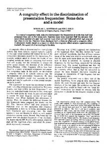
ods of reconstruction and estimated uncertainties can be found in Budyko (1988), Velichko (1985), Zubakov (1990) and Borzenkova (1992). For the reconstruction of the Mid-Pliocene temperature over NH land, various proxy data from 80 key cross-sections (see references in Borzenkova, 1992) were used to reconstruct the landscapes first (Zubakov, 1990; Zubakov and Borzenkova, 1988, 1990), after which the temperature was estimated with a landscapephytocenological model developed by Sinitsyn (1967, 1969, 1980) and Khotinsky and Savina (1985). The resulting spatial reconstruction was refined by integrating 12 direct estimates of temperature obtained by Liberman et al. (1985) from their statistical model that relates spore-pollen spectra with temperature and precipitation. The reconstruction B of the Mid-Pliocene SST is based on the relationship between modern assemblages of planktonic foraminifera and SST (Be, 1977; Os’kina et al., 1982; Velichko, 1985; Barash et al., 1987; Blum et al., 1987). The change of planktonic zones in the Mid-Pliocene was estimated from the data by Bandy et al. (1971), Berggren and Van Covering (1974) and Keller (1979) and from the extensive database of Blum and co-workers (Blum, 1982; Blum et al., 1987). The Mid-Pliocene gridded summer and winter temperature reconstructions B are reproduced in Figure 1. The largest temperature anomalies in the Pliocene time occur in winter over the north-east of Asia and the Canadian Arctic Islands. The evidence for such large climate changes in these regions is based on paleobotanical data (Biske, 1975; Fradkina, 1983; Phanerozoic of Siberia, 1984; Fot’janova, 1987). According to these sources, in the Early-Middle Pliocene on the coast of the Arctic the birchalder-larch forests predominated, which indicates that the winter temperatures were 15–20 ◦ C above their modern values. The absence of the permanent seaice in the Arctic (Herman and Hopkins, 1980; Danilov, 1987; Thompson, 1991) and a considerable reduction of the continental permafrost area (Thompson, 1991; Velichko and Nechaev, 1992) points to the same range of temperature anomaly in these regions (Zubakov and Borzenkova, 1988, 1990). The summer cooling over the present-day Sahara is also inferred from the changed landscape. The desert area was reduced (Leroy and Dupont, 1994) and replaced by savannah with numerous lakes (Bonnefille et al., 1987); the area of the African rainforest was significantly larger (Williamson, 1985). This is indicative of a Pliocene cooling of about 1–3 ◦ C over the Sahara region. Figure 1 also shows a winter cooling over the north-eastern North Atlantic and northern Europe, which may be attributed to a difference in oceanic circulation caused by the fact that in the Mid-Pliocene the Panama Gateway was not completely closed (Zubakov and Borzenkova, 1990). The estimate of precipitation in the Mid-Pliocene by Borzenkova is based on combination of temperature and landscape reconstructions (Sinitsyn, 1967, 1969; Zubakov, 1990), in which the present-day empirical relationship between annual temperature, evapotranspiration and precipitation within a given landscape by Zubenok (1975) was used for estimating the annual sum of precipitation. At 12
698
M. V. SHABALOVA ET AL.
Figure 1. Reconstruction of the Mid-Pliocene summer (JJA) and winter (DJF) temperature anomalies by Borzenkova (1992). The isoline increment is 2 ◦ C.
sites the reconstruction was supplemented with direct estimates of precipitation from spore-pollen spectra by Liberman et al. (1985). According to Klimanov (1985) and Grichuk (1985), the uncertainty of the precipitation reconstruction in the two Pleistocene epochs is about 25 mm/year (∼0.07 mm/day) per gridpoint; that in the Mid-Pliocene is estimated by the author (IIB) to be roughly 50 mm/year (∼0.14 mm/day). However, the uncertainty of reconstruction of the Mid-Pliocene precipitation is difficult to assess because the method is indirect, involving the reconstruction of the landscapes and temperatures from proxy data as a first step. Over North America the reconstruction is less reliable due to scarcity of the proxy data; over the former U.S.S.R. and Alaska the reconstruction is more accurate than elsewhere because of the inclusion of direct estimates by Liberman et al. (1985). Supporting evidence for putting confidence in well-marked zonal-scale features of precipitation reconstruction B in Pliocene comes from the reasonable agree-
PRECIPITATION CHANGE: MODEL SIMULATIONS AND PALEORECONSTRUCTIONS
699
TABLE I Averaged climatic parameters for the Northern Hemisphere (NH). TNH is the NH-averaged annual-mean temperature; PNH is the NH-averaged precipitation over land. Present-day precipitation rates and temperatures are from Jaeger (1983) and Oort (1983) respectively. Paleodata are reconstructions by Borzenkova (1992) for three past warm epochs: Mid-Holocene, Eemian and Mid-Pliocene. The model data are from GFDL and UKHI high-resolution GCMs (see the text). The lower panel gives the changes with respect to present for paleodata and the anomalies from perturbation (2 × CO2 ) equilibrium response experiments with respect to control (1 × CO2 ) runs. Precipitation changes separately for tropics (0–30 N) and extratropics (30–70 N) are also shown Present
Holocene
Eemian
Pliocene
GFDL
15.3 2.17 2.91 1.41
16.3 2.50 3.42 1.57
17.1 2.63 3.47 1.77
18.9 2.68 3.47 1.87
control (1 × CO2 ) 11.7 13.2 2.73 2.08 3.65 2.63 1.53 1.41
1TNH (◦ C) 1PNH (%) 1P0−30 N (%) 1P30−70 N (%)
1.0 15 18 11
1.8 21 19 26
3.6 24 19 33
2 × CO2 –1 × CO2 3.8 3.8 13 10 10 10 19 12
1PNH /1TNH (%/◦ C)
15
12
TNH (◦ C) PNH (mm/day) P0−30 N (mm/day) P30−70 N (mm/day)
7
3
UKHI
3
ment in zonal patterns of temperature change in reconstructions B and D (Section 3), combined with the fact that a modeling study of Mid-Pliocene by Sloan et al. (1996), in which the model, being forced with SST from reconstruction D, shows features over land which are consistent with Borzenkova’s temperature and precipitation reconstructions. Table I lists the values of the NH-averaged surface temperature anomaly, 1TNH , calculated as half of sum of winter and summer temperatures, and the precipitation anomaly over NH land, 1PNH , for the three past warm climates. 2.2.
MODEL DATA
In different models, the equilibrium response to CO2 doubling varies in a large range, even in terms of global averages. For globally-averaged surface air temperature and annual precipitation anomalies the ranges are 1.5–4.5 ◦ C and 4–15% respectively (IPCC, 1990, 1996; Boer, 1993). For zonal averages, the scatter in model results increases and remains present even if models with equal sensitiv-
700
M. V. SHABALOVA ET AL.
ity of global temperature to CO2 doubling are compared. To reduce part of the uncertainty, we selected for this study as a model baseline two GCMs of equal (high) resolution and of equal sensitivities of both global temperature and global precipitation in standard 2 × CO2 equilibrium experiments. The selected models are the Geophysical Fluid Dynamics Laboratory high-resolution GCM (GFDL) and Hadley Centre’s high-resolution GCM (UKHI). The GFDL model output (Manabe and Wetherald, 1990) is available from the NCAR Data Support Section (R30 runs). The output of the Hadley Centre’s climate model (UKHI, R30 runs) is available from the Hadley Centre for Climate Prediction and Research (Mitchell et al., 1989). In both GCMs, the monthly mean surface air temperature and precipitation fields are 10-years averages from the mixed layer ocean model control run and from the standard equilibrium 2 × CO2 experiment. The fields have a spatial resolution of approximately 2.2 degrees in latitude and 3.75 degrees in longitude. In both GCMs the sensitivity of NH-averaged temperature to the doubling of CO2 concentration is 3.8 ◦ C and the sensitivity of NH-averaged precipitation over land is about 12% (Table I).
3. Pliocene Temperature Patterns Figure 2 compares the Pliocene zonally-averaged seasonal SSTs in reconstructions B and D. To obtain absolute values of SST from reconstruction B, the temperature anomalies B were first averaged zonally at sea gridpoints and then these values were added to the present-day zonally averaged seasonal climatology by Oort (1983). Although the two Mid-Pliocene reconstructions refer to different time slices, the zonal patterns of seasonal temperature change of these two independent reconstructions compare well, showing both of them small changes in tropics and enhanced warming northward. The most marked discrepancies between B and D appear in summer at mid-latitudes (∼ 3◦ C) and in winter at high latitudes. In the data-lacking polar region, reconstructions B and D diverge further, as D assigns the present-day values to the Arctic temperatures while B indicates a pronounced warming here. According to Budyko et al. (1985), reconstruction B refers to a warmer period of the Pliocene than reconstruction D, but from the ocean-only reconstructions in Figure 2 this is not apparent, since both reconstructions result in comparable values of hemispherically-averaged temperature. Now we compare the temperature response as simulated by two GCMs considered here in their 2 × CO2 –1 × CO2 equilibrium experiments with that in reconstruction B of the Mid-Pliocene. To approximate the annual-means, the summer and winter temperature anomalies in the reconstruction and in the models were averaged at each gridpoint and then averaged zonally/hemispherically. Table I shows, among other data, the NH-averaged warming 1TNH for the two GCMs and the Mid-Pliocene. In both models 1TNH = 3.8 ◦ C, for the Mid-Pliocene 1TNH = 3.6 ◦ C. This would be a perfect agreement if the warmth in the Mid-Pliocene were due to a
PRECIPITATION CHANGE: MODEL SIMULATIONS AND PALEORECONSTRUCTIONS
701
Figure 2. The Mid-Pliocene zonally-averaged SST for summer and winter as reconstructed by Borzenkova (1992) compared with the Pliocene reconstruction by Dowsett et al. (1996). The present-day climatology over the ocean (Oort, 1983) is also shown. This climatology has been used to transform the temperature anomalies of Borzenkova’s reconstruction into absolute values. All curves represent zonally-averaged values at ocean gridpoints.
702
M. V. SHABALOVA ET AL.
Figure 3. Zonally-averaged (land+ocean) annual-mean temperature anomalies dT scaled with the NH-averaged warming 1TNH , as reconstructed for the Mid-Pliocene and as simulated by two general circulation models. The paleodata are the reconstruction of air surface temperature anomalies by Borzenkova (1992). Simulated data are changes from two separate control (1 × CO2 ) and perturbation (2 × CO2 ) equilibrium response experiments. The model outputs are from Geophysical Fluid Dynamics Laboratory high-resolution GCM (GFDL) and from Hadley Centre’s high-resolution GCM (UKHI).
doubling of CO2 , but as the Mid-Pliocene CO2 level has been only 30% above the pre-industrial level, then the Mid-Pliocene climate response to radiative forcing has been much stronger than the two models imply. Part of this excessive warmth may have resulted from internal climatic processes amplifying the greenhouse signal (Rind and Chandler, 1991; Raymo et al., 1996). Leaving aside the question about other possible causes of the Mid-Pliocene warmth and assuming that it was indeed solely due to 30% increase of CO2 , then the paleodata suggest that the ultimate sensitivity of temperature to CO2 doubling is about three times larger than it was previously accepted based on model experiments. Figure 3 compares the zonally-averaged annual-mean temperature anomalies dT from the two GCMs with the Mid-Pliocene. The anomalies are normalized by the corresponding value of 1TNH . The two Pleistocene optima are not included in the Figure, but earlier studies (Budyko, 1988; Hoffert and Covey, 1992; Shabalova and Können, 1995) indicate that the 1TNH -normalized zonal temperatures of these epochs are similar to those of the Mid-Pliocene. The model-based curves agree with each other at low-to-mid latitudes but diverge at high latitudes. Compared to
PRECIPITATION CHANGE: MODEL SIMULATIONS AND PALEORECONSTRUCTIONS
703
the Mid-Pliocene (and two other epochs), the models distribute the warming more evenly over the latitudes; the largest contribution to the value of global warming in the models originates from low latitudes. Figure 3 is illustrative of the fact that on zonal scale there is a persistent difference between model and paleo patterns of temperature changes (see also Crowley, 1993).
4. Precipitation Patterns 4.1.
PRECIPITATION IN
GCMS
Although the hydrological cycle is only a secondary feature of the general circulation, the control-climate experiments are able to reproduce satisfactorily the globally/hemispherically-averaged rates of precipitation. For the two selected models the globally-averaged precipitation rate is 2.8 mm/day, which agrees with the empirical estimate of 2.7 mm/day (Jaeger, 1983). At smaller spatial scales the agreement deteriorates. The biases in simulated control-climate temperature (up to 5 ◦ C for zonal averages) are translated to even larger biases in regional precipitation. Table I indicates that for the precipitation averaged over the land areas in the NH the disagreement between the control-climate simulations and observations reaches 25%. In 2 × CO2 –1 × CO2 equilibrium response experiments all the models indicate an increase of precipitation on a global scale. According to Boer (1993), the sensitivity of global annual precipitation to global temperature change in the GCMs varies between 1%/◦ C and 3%/◦ C, with a mean value of 2%/◦ C, which is 0.05 mm/day or 20 mm/year per 1 ◦ C of global warming. In both selected models this sensitivity is about 3%/◦ C; the sensitivity of NH-averaged land-only precipitation to the hemispheric warming is also 3%/◦ C (Table I). Figure 4 shows the zonal distributions of absolute precipitation anomalies over land dP, simulated by the two models. A visual inspection of the GCMbased curves of the Figure 4 indicates good agreement in the tropics and at about 50–70 N. Between 20 and 50 N the between-model difference in simulated precipitation anomalies is large. 4.2.
PALEO PRECIPITATION
Figure 4 shows also the zonal averages of reconstructed precipitation anomalies dP over NH land in the Mid-Pliocene and the two Pleistocene optima. The three paleocurves exhibit a typical pattern of change, showing a peak at about 20 N (the area of the modern subtropical deserts) and an increase of precipitation from midto high latitudes, where the zonal warming (see Figure 3 for the Mid-Pliocene, and Figure 1 in Shabalova and Können (1995) for the two other epochs) is largest. Averaged over the NH land area, the precipitation rises with warming, but this dependence levels off with increasing warmth (Table I). The sensitivity of
704
M. V. SHABALOVA ET AL.
Figure 4. Zonally-averaged annual-mean precipitation anomalies dP (mm/day) over NH land, reconstructed and simulated. Paleodata are changes from present in the three warm climates: Mid-Holocene, Eemian and Mid-Pliocene (Borzenkova, 1992). The error bars (shown at one point in each paleocurve) indicate the estimated uncertainty per gridpoint in the three paleoreconstructions. Simulated data are changes between 1 × CO2 and 2 × CO2 equilibrium response experiments.
hemispheric precipitation to hemispheric warming 1PNH /1TNH is 15%/◦ C if the Mid-Holocene is compared with present (1TNH = 1 ◦ C) but drops to 7%/◦ C if Mid-Pliocene is compared with present (1TNH = 3.6 ◦ C). Figure 4 shows that the dependence of precipitation on temperature originates mainly from the extratropics, as the desert-belt peak in paleo precipitation shows little sensitivity to the between-epoch differences in global warming. Within the uncertainty of the reconstructions, the increase in precipitation in the φ < 30 N belt is for all three epochs the same. In the 30 ≤ φ ≤ 70 N latitudinal belt, the sensitivity of precipitation to 1TNH has a value of about 15%/◦ C if Mid-Holocene, Eemian and present are compared, which is considerably higher than the 4%/◦ C response indicated by the two models (Figure 5). On the other hand, if Eemian is compared with Mid-Pliocene, the precipitation response in the 30–70 N belt is only 4%/◦ C. The high value of paleo precipitation anomaly over the modern desert-belt and its insensitivity to 1TNH can be understood from a long-term adjustment of the soil moisture, vegetation, and hence the local hydrological cycle, to a new equilibrium (Cunnington and Rowntree, 1986; Lapenis and Shabalova, 1994; Lofgren, 1995). An increase in monsoon areas of the moisture advected from the warmer ocean initiates a transition of the landscape from dry to more humid. This results in a change of the surface albedo and, even more importantly, in an increase of the
PRECIPITATION CHANGE: MODEL SIMULATIONS AND PALEORECONSTRUCTIONS
705
Figure 5. Response of extratropical precipitation (30–70 N belt) over land to hemispheric warming 1TNH in epochs and models. The dots represent estimates of precipitation increase in Mid-Holocene, Eemian and Mid-Pliocene with respect to present. The model estimates (crosses) are changes from 1 × CO2 and 2 × CO2 equilibrium response experiments.
water holding capacity of the soil layer. The changes in surface properties enhance local evaporation and hence local precipitation. Paleo evidence (Street-Perrot and Perrot, 1993) and modeling studies (Texier et al., 1997; Ganopolski et al., 1998) indicate that even the Mid-Holocene level of warming was sufficient to result in a substantial contraction of the Sahara area. The intensification of the local hydrological cycle over the desert belt is accompanied by a decrease of land surface temperatures due to evaporative cooling (see Figure 1). This cooling results in a decrease of land-sea temperature contrast, which is the main driving force for the monsoon. Hence, with progressing warming, this negative precipitation-temperature feedback may account for the observed stability of the desert-belt peak in precipitation for paleoclimates with 1TNH in the range 1–4 ◦ C.
5. Model/Paleodata Comparison The desert-belt peak in paleo precipitation is not reproduced in the doubled CO2 model experiments. This is to be expected, because GCMs in their standard perturbed experiments do not account for the change of vegetation or soil properties and hence do not reproduce the intensification of the local hydrological cycle and
706
M. V. SHABALOVA ET AL.
the associated regional cooling. The longest time scale which determines the equilibrium in GCMs refers to the mixed-layer ocean adjustment. In this sense, the equilibria of models and of paleodata represent different states. A recent modelling study by Kutzbach et al. (1996) points the way for the model/paleodata convergence in the area of modern deserts. North of the subtropical desert belt there exists some similarity between the zonally-averaged precipitation anomalies in models and in paleoclimates (Figure 4). The anomalies simulated by the GFDL model fall in the range implied by the reconstructions of the three climates. The UKHI-based curve lies out of this range in the 30-50 N belt, but at higher latitudes the reconstructed and simulated anomalies are in qualitative agreement. The simulated anomalies are, however, systematically lower than the anomalies of the Mid-Pliocene, which is the epoch with comparable level of hemispheric warming. Rescaling the model anomalies down to account for a Mid-Pliocene level of 1.3 × CO2 increases the model/paleodata discrepancy. The sensitivity of precipitation averaged over land area north of 30 N to hemispheric warming is about 4%/◦ C in the models versus 9%/◦ C in Mid-Pliocene (Figure 5). To assess quantitatively the degree of similarity in the spatial anomaly patterns of the simulations and paleo reconstructions we first interpolate the model outputs into the paleo grid and then calculate the spatial pattern cross-correlation coefficient C (Santer et al., 1993): P δA1 (x) · δA2 (x) C= x (1) δA1 (x) · δA2 (x) Here x is the space coordinate (grid-points); pδA Pi (x) are the2 gridded uncentered climatic anomalies of two fields; δAi (x) = x (δAi (x)) . Table II shows the model/paleodata pattern cross-correlations for the change of precipitation together with the between-model and between-epoch correlations. The numbers in bold represent precipitation-temperature pattern correlations for each individual epoch and model. Due to the large between-model divergence of simulated precipitation anomalies over 20–50 N, the model-to-model spatial correlation in change of precipitation is only 0.4. The epoch-to-epoch correlations are much stronger, 0.8–0.9. The patterns of temperature and precipitation changes are positively correlated in the models and in the reconstructions, which is a likely result of the increase of the available atmospheric moisture. Table II indicates that the warmer the paleoclimate is, the stronger the precipitation-temperature correlation: C increases from 0.4 for the Mid-Holocene to 0.7 for the Mid-Pliocene. This difference can be attributed to the weak response of precipitation to warming in the 40–60 N belt in Mid-Holocene. In both models the values of the precipitation-temperature pattern correlations are small and smaller even than the value for the Mid-Holocene. The two model-based precipitation signals have the highest expression in the data from the Mid-Pliocene; the correlations are the lowest with the Mid-Holocene
PRECIPITATION CHANGE: MODEL SIMULATIONS AND PALEORECONSTRUCTIONS
707
TABLE II Model-to-epoch, model-to-model and epoch-to-epoch spatial pattern correlations C (Equation (1)) for changes in annual-mean precipitation. Model data are changes from the control (1 × CO2 ) and perturbation (2 × CO2 ) equilibrium response experiments. Paleodata are changes from present in the three past warm climates. The figures in bold font are the correlations between temperature and precipitation patterns for each model and epoch Epoch–model
UKHI
GFDL
Holocene
Eemian
Pliocene
Holocene Eemian Pliocene
0.45 0.54 0.52
0.62 0.74 0.81
0.41 0.90 0.83
0.58 0.94
0.66
UKHI GFDL
0.34 0.43
0.27
precipitation field. On the average, the model/paleodata spatial correlations for changes in precipitation are 0.5 for the UKHI model, and about 0.7 for the GFDL model (Table II). Outside the tropics the correlations are somewhat higher; for the 30–70 N belt the values are 0.6 and 0.8 respectively.
6. Summary and Conclusions Comparison of reconstructions of three warm past epochs shows similarities in the spatial patterns of precipitation change (Figure 4, Table II). Paleo precipitation anomaly pattern shows a marked peak in the area of the modern subtropical deserts and an increase of precipitation from mid- to high latitudes, where the zonal warming is largest (Figures 1 and 3). The epoch-to-epoch spatial correlations for changes in precipitation exceed 0.8 (Table II). With respect to present, the response of the NH-averaged precipitation over land to hemispheric warming, 1PNH /1TNH , is 15, 12 and 7%/◦ C for the Mid-Holocene, Eemian and Mid-Pliocene respectively (Table I). The precipitation-temperature relation weakens with warming partly due to an epoch-independent precipitation response in the subtropical desert-belt (Figure 4). North of the desert-belt, the response of precipitation to 1TNH has a value of about 15%/◦ C if Mid-Holocene, Eemian and present are compared; the response is 4%/◦ C if Eemian is compared with Mid-Pliocene (Figure 5). Comparison of precipitation fields simulated by two GCMs with equal sensitivity of the NH-averaged temperature and precipitation to CO2 doubling in standard (2 × CO2 -1 × CO2 ) equilibrium experiments shows a large scatter of the results on zonal scale (Figure 4). The model-to-model spatial correlation in change of
708
M. V. SHABALOVA ET AL.
precipitation is 0.4 (Table II). The sensitivity of the NH-averaged precipitation over land to hemispheric warming is in both models 3%/◦ C (Table I). Model/paleodata comparison shows that the largest differences in precipitation patterns arise in the present-day desert-belt (Figure 4). This disagreement stems likely from the fact that the standard model experiments do not include the slow soil-vegetation-precipitation feedback, which is crucially important here. This feedback provides an increase of precipitation as well as paleo cooling (Figure 1) in this region in summer. North of 50 N the absolute zonal values of simulated precipitation anomalies are in the range implied by the three paleoclimates. However, although the simulated hemispheric warming is comparable with the Mid-Pliocene, the simulated precipitation anomalies are systematically lower than those in the Mid-Pliocene (Figure 4); also the temperature anomalies north of 50 N are in the models lower than those in the Mid-Pliocene (Figure 3). Rescaling the model anomalies from 2 × CO2 to a Mid-Pliocene level of 1.3 × CO2 increases the model/paleodata discrepancy. If our reconstructions are valid and if climate changes in the Mid-Pliocene were driven solely by CO2 changes, then our results suggest that models are underestimating the magnitude of the precipitation response to radiative forcing as well as to hemispheric warming, especially in the subtropical desert-belt, and that they are underestimating the magnitude of the temperature response at high latitudes. At least part of the reported model/paleodata discordance appears to be due to lack of interactive land surface package in the models examined. Another part may be attributed to differences in boundary conditions in a past climate as compared to the experimental model design. Modification of a number of input parameters/fields, including specification of the SST (Sloan et al., 1996) turns out to improve the agreement of simulated Mid-Pliocene climate with the paleoreconstruction. On the other hand, the ocean is an interactive part of the climatic system in a wide range of timescales. A recent modelling study by Bush and Philander (1998) indicates that a coupled atmosphere-ocean GCM configured for a past epoch by specifying only external forcings is indeed capable to deliver a consistent picture of a past climate. Accounting for oceanic circulation and dynamical ocean-atmosphere interactions turns out to be of crucial importance for simulating realistic climates. Some of the conclusions of the present study rely on features in the paleoreconstructions that are close to the limit of reliability. Although certain features in our reconstructions are solid, the possibility remains that our main results – the epoch-to-epoch similarity in patterns of precipitation change, the large sensitivity of precipitation to warming and the model/paleodata disagreement – are artificially amplified by flaws in the methodologies of inferring climatic information from paleo proxy records. On the other hand, the between-model difference in patterns of precipitation and high-latitude temperature change, as simulated in identical sensitivity experiments, leaves room for the models’ convergence. A new generation of coupled climate models with fully dynamic oceans can provide a basis for the
PRECIPITATION CHANGE: MODEL SIMULATIONS AND PALEORECONSTRUCTIONS
709
improvement of the paleo proxies interpretation. And vice versa, the models will gain in performance through the calibration against enhanced paleoreconstructions.
Acknowledgements We thank A. Oort for providing his gridpoint climatology and D. Viner and R. Stouffer for their assistance in model data retrieval. The incisive comments of anonymous reviewers are highly appreciated.
References Bandy, O. L., Casey, R. E., and Wright, R. C.: 1971, ‘Late Neogene Planktonic Zonation, Magnetic Reversals and Radiometric Dates: Antarctic to Tropics’, Antarc. Oceanol. 1, 1–26. Barash, M. S., Kuptsov, V. M., and Os’kina, N. S.: 1987, ‘The Atlantic: The New Data about Chronology of Late Pleistocene and Holocene’, Bull. Quat. Stud. 56, 3–10 (in Russian). Barnett, T. P., Santer, B. D., Jones, P. D., Bradley, R. S., and Briffa, K. R.: 1996, ‘Estimates of Low Frequency Variability in Near-Surface Air Temperature’, The Holocene 6, 255–263. Be, A. W. H.: 1977, ‘An Ecologic, Zoogeographic and Taxonomic Review of Recent Planctonic Foraminifera’, Ocean. Micropaleontol. 1. Berggren, W. A. and Van Covering, J.: 1974, ‘The Late Neogene. Biostratigraphy, Geochronology and Paleoclimatology of the Last 15 Million Years in Marine and Continental Sequences’, Palaeogeogr. Palaeoclimatol. Palaeoecol. 16, 1–216. Biske, S. F.: 1975, The Paleogene and Neogene of the Extreme North-East of the USSR, Nauka, Novosibirsk, p. 168. Blum, N. S.: 1982, Paleotemperature Reconstructions in Different Regions of World Ocean for Pleistocene, Based on Planktonic Foraminifers Data, Aftoreferat dissertatsii, Moscow, p. 24 (in Russian). Blum, N. S., Ivanova, E. V., and Os’kina, N. S.: 1987, ‘Reconstruction of the Climatic Ocean Zonality (By Using Foraminifer Data)’, in Earth’s Climate in the Geological Time, Nauka, Moscow, pp. 125–140 (in Russian). Boer, G.J.: 1993, ‘Climate Change and the Regulation of the Surface Moisture and Energy Budgets’, Clim. Dyn. 8, 225–239. Boer, G. J., Arpe, K., Blackburn, M., Deque, M., Gates, W. L., Hart, T. L., Le Treut, H., Roeckner, E., Sheinin, D. A., Simmonds, I., Smith, R. N. B., Tokioka, T., Wetherald, R. T., and Williamson, D.: 1992, ‘Some Results from an Intercomparison of the Climates Simulated by 14 Atmospheric General Circulation Models’, J. Geophys. Res. 97, 12771–12786. Bonnefille, R., Vincens, A., and Buchet, G.: 1987, ‘Palynology, Stratigraphy and Palaeoenvironment of a Pliocene Hominid Site (2.9–3.3 M.Y.) at Hodar, Ethiopia’, Palaeogeogr. Palaeoclimatol. Palaeoecol. 60, 249–281. Borzenkova, I. I.: 1992, The Changing Climate during the Cenozoic, Hydrometeoizdat, St. Petersburg, p. 247 (in Russian). English translation by Yanuta, V. G.: U.S.-Russian Workshop ‘Paleocalibration of Climate Sensitivity’, 15–17 August, 1994, Printed under the Auspices of Working Group VIII: The Influence of Environmental Changes on Climate, U.S.-Russian Agreement on Cooperation in the Field of Environmental Protection. Bradley, R. S.: 1986. Quaternary Paleoclimatology, Winchester, Allen and Unwin, p. 472. Budyko, M. I.: 1988. Anthropogenic Climate Change, D.Reidel, Dordrecht, p. 460.
710
M. V. SHABALOVA ET AL.
Budyko, M. I., Ronov, A. B., and Yanshin, A. L.: 1985. History of the Earth’s Atmosphere, Springer, p. 137. Bush, A. B. G. and Philander, S. G. H.: 1998, ‘The Role of Ocean-Atmosphere Interactions in Tropical Cooling during the Last Glacial Maximum’, Science 279, 1341–1344. Cess, R. D., et al.: 1990, ‘Intercomparison and Interpretation of Climate Feedback Processes in 19 Atmospheric General Circulation Models’, J. Geophys. Res. 95, 16601–16615. CLIMAP Project Members: 1976, ‘The Surface of the Ice Age Earth’, Science 191, 1131–1137. CLIMAP Project Members: 1984, ‘The Last Interglacial Ocean’, Quatern. Res. 21, 123–224. COHMAP Members: 1988, ‘Climatic Changes of the Last 18,000 Years: Observations and Model Simulations’, Science 241, 1043–1052. Covey, C.: 1995, ‘Using Paleoclimates to Predict Future Climate: How Far Can Analogy Go?’, Clim. Change 29, 403–407. Crowley, T. J.: 1991, ‘Modeling Pliocene Warmth’, Quatern. Sci. Rev. 10, 275–282. Crowley, T. J.: 1993, ‘Geological Assessment of the Greenhouse Effect’, Bull. Amer. Meteorol. Soc. 74, 2363–2373. Crowley, T. J.: 1996, ‘Pliocene Climates: The Nature of the Problem’, Mar. Micropaleontol. 27, 3–12. Crowley, T. J. and North, G. R.: 1991, Paleoclimatology, Oxford Univ. Press, Clarendon Press, Oxford, p. 360. Cunnington, W. M. and Rowntree, P. R.: 1986, ‘Simulation of the Sahara Atmosphere – Dependence on Moisture and Albedo’, Quart. J. Roy. Meteorol. Soc. 112, 971–999. Danilov, I. D.: 1987, ‘The History of Development the Cryolithozone in Northern Eurasia in the Late Cenozoic’, in Geocryological Studies, Moscow (in Russian). Dowsett, H. J., Barron, J., and Poore, R.: 1996, ‘Middle Pliocene Sea Surface Temperatures: A Global Reconstruction’, Mar. Micropaleontol. 27, 13–26. Fot’janova, L. I.: 1987, ‘Climate over the Continental Regions Bordering the Pacific Ocean during the Cenozoic’, in: Earth Climate in Geological Time, Nauka, Moscow, pp. 95–124 (in Russian). Fradkina, A. F.: 1983. The Neogene Palinoflora of North-Eastern Asia, Nauka, Moscow, p. 223 (in Russian). Ganopolski, A., Kubatzki, C, Claussen, M, Brovkin, V. and Petoukhov, V.: 1998, ‘The Influence of Vegetation-Atmosphere-Ocean Interaction on Climate during the Mid-Holocene’, Science 280, 1916–1919. Grichuk, V. P.: 1985: ‘Reconstructions of Climatic Parameters by Floristic Data and Assessment of their Accuracy’, in Velichko, A. A., Serebrjannyi, L. R., and Gurtovaja, E. E. (eds.), Methods of Reconstructions of Paleoclimates, Nauka, Moscow, pp. 20–28 (in Russian). Hartmann, D. L. and Michelsen, M. L.: 1993, ‘Large-Scale Effects on the Regulation of Tropical Sea Surface Temperature’, J. Climate 6, 2049–2060. Herman Y. and Hopkins D. M.: 1980, ‘Arctic Oceanic Climate in the Late Cenozoic Time’, Science 209, 557–562. Hoffert, M. I. and Covey, C.: 1992, ‘Deriving Global Climate Sensitivity from Palaeoclimate Reconstructions’, Nature 360, 573–579. Hurrell, J. W.: 1995, ‘Comparison of NCAR Community Climate Model (CCM) Climates’, Clim. Dyn. 11, 25–50. Intergovernmental Panel on Climate Change (IPCC): 1990, Climate Change, The IPCC Scientific Assessment, Houghton, J. T., Jenkins, G. J., and Ephraums, J. J. (eds.), Cambridge Univ. Press, Cambridge, U.K., p. 365. Intergovernmental Panel on Climate Change (IPCC): 1996, Climate Change 1995: The Science of Climate Change, Houghton, J. T., Meira Filho, L. G., Callander, B. A., Harris, N., Kattenberg, A., and Maskell, K. (eds.), Cambridge Univ. Press, Cambridge, U.K., p. 572. Jaeger, L.: 1983, ‘Monthly and Areal Patterns of Mean Global Precipitation’, in Street-Perrot, A., Beran, M., and Radcliff, R. (eds.), Variation of the Global Water Budget, D. Reidel Publ., Dordrecht, pp. 120–140.
PRECIPITATION CHANGE: MODEL SIMULATIONS AND PALEORECONSTRUCTIONS
711
Joussaume, S. and Taylor, K. E.: 1995, ‘Status of the Paleoclimate Modeling Intercomparison Project’, in Proceedings of the First International AMIP Scientific Conference, Monterrey, U.S.A, WCRP-92, pp. 425–430. Keller, G.: 1979, ‘Late Neogene Paleoceanography of the North Pacific DSDP Sites 173, 310 and 296’, Mar. Micropaleontol. 4, 159–172. Khotinsky, N. A. and Savina, S. S.: 1985, ‘Paleoclimatic Maps of the U.S.S.R. Territory in Boreal, Atlantic and Subboreal Periods of the Holocene’, Ann. Acad. Sci. U.S.S.R., Ser. Geogr. 4, 18–34 (in Russian). Kim, K.-Y., North, G. R., and Hegerl, G. C.: 1996, ‘Comparisons of the Second-Moment Statistics of Climate Models’, J. Climate 9, 2204–2221. Klimanov V. A.: 1985, ‘The Reconstructions of the Paleotemperature and Paleo Precipitation by Using Pollen Data’, in Velichko, A. A., Serebrjannyi, L. R., and Gurtovaja, E. E. (eds.), Methods of Reconstructions of Paleoclimates, Nauka, Moscow, pp. 38–48 ( in Russian). Kutzbach, J. E., Bonan, G., Foley, J., and Harrison, S. P.: 1996, ‘Vegetation and Soil Feedbacks on the Response of the African Monsoon to Orbital Forcing in the Early to Middle Holocene’, Nature 384, 623–626. Kutzbach, J. E., Guetter, P. J., Behling, P. J., and Selin, R.: 1993, ‘Simulated Climatic Changes: Results of the COHMAP Climate-Model Experiments’, in Wright, H. E. et al. (eds.), Global Climate Since the Last Glacial Maximum, University of Minnesota Press, pp. 24–93. Lapenis, A. G. and Shabalova, M. V.: 1994, ‘Global Climate Changes and Moisture Conditions in the Intracontinental Arid Zones’, Clim. Change 27, 283–297. Lau, K.-M., Kim, J. H., and Sud, Y.: 1996, ‘Intercomparison of Hydrologic Processes in AMIP GCMs’, Bull. Amer. Meteorol. Soc. 77, 2209–2227. Leroy S. and Dupont L.: 1994, ‘Development of Vegetation and Continental Aridity in NorthWestern Africa during the Late Pliocene: The Pollen Record of ODP Site 658’, Palaeogeogr. Palaeoclimatol. Palaeoecol. 109, 295–316. Liberman, A. A., Muratova, M. V., and Suetova, I. A.: 1985, ‘A Non-Linear Interpolation Method for Developing the Paleoclimate Models’, in Velichko, A. A., Serebrjannyi, L. R., and Gurtovaja, E. E. (eds.), Methods of Reconstructions of Paleoclimates, Nauka, Moscow, pp. 48–53. Lofgren, B. M.: 1995, ‘Sensitivity of Land-Ocean Circulations, Precipitation, and Soil Moisture to Perturbed Land Surface Albedo’, J. Climate 8, 2521–2562. Manabe, S. and Wetherald, R. T.: 1990, reported in Mitchell, J. F. B., Manabe, S., Meleshko, V., and Tokioka, T. ‘Equilibrium Climate Change – and its Implications for the Future’, in Houghton, J. T., Jenkins, G. J., and Ephraums, J. J. (eds.), Climate Change: The IPCC Scientific Assessment, Cambridge University Press, Cambridge, U.K., pp. 131–172. Mitchell, J. F. B., Senior, C. A., and Ingram, W. J.: 1989, ‘CO2 and Climate: A Missing Feedback?’, Nature 341, 132–134. Oort, A.: 1983, Global Atmospheric Circulation Statistics, NOAA Professional Paper No.14, Washington D.C., p. 180. Os’kina, N. S., Ivanova, E. V., and Blum, N. S.: 1982, ‘Climatic Zonality of the Atlantic, Indian and Pacific Oceans in the Pliocene’, Ann. Acad. Sci. USSR 264, N2, 400–407 (in Russian). Phanerozoic of Siberia, Mesozoic and Cenozoic: 1984, Proc. Inst. of Geology and Geophysics, Vol. 596, Novosibirsk (in Russian). Raymo, M. E., Grant, B., Horowitz, M., and Rau, G. H.: 1996, ‘Mid-Pliocene Warmth: Stronger Greenhouse and Stronger Conveyor’, Mar. Micropaleontol. 27, 313–326. Rind, D. and Chandler, M.: 1991, ‘Increased Ocean Heat Transport and Warmer Climate’, J. Geophys. Res. 96, 7437–7461. Santer, B. D., Wigley, T. M. L., and Jones, P. D.: 1993, ‘Correlation Methods in Fingerprint Detection Studies’, Clim. Dyn. 8, 265–276. Shabalova, M. V. and Können, G. P.: 1995, ‘Climate Change Scenarios: Comparisons of Paleoreconstructions with Recent Temperature Changes’, Clim. Change 29, 409–428.
712
M. V. SHABALOVA ET AL.
Shabalova, M. V. and Können, G. P.: 1995a, ‘Scale Invariance in Long-Term Time Series’, in Novak, M. M. (ed.), Fractal Reviews in the Natural and Applied Sciences, Chapman and Hall, pp. 309– 319. Sinitsyn, V. M.: 1967, Introduction in Paleoclimatology, Nedra, Leningrad, p. 232 (in Russian). Sinitsyn, V. M.: 1969, ‘A Geologic Method of the Paleoclimatic Reconstructions’, Izd. LGU 1, 55–63 (in Russian). Sinitsyn, V. M.: 1980, Natural Conditions and Climate over the U.S.R.R. Territory in the Early and Middle Cenozoic, Hydrometeoizdat, Leningrad, p. 103 (in Russian). Sloan, L. C., Crowley, T. J., and Pollard, D.: 1996, ‘Modelling of Middle Pliocene Climate with the NCAR GENESIS General Circulation Model’, Mar. Micropaleontol. 27, 51–61. Street-Perrot, A. F. and Perrot, R. A.: 1993, ‘Holocene Vegetation, Lake Levels and the Climate of Africa’, in Wright, H. E. et al. (eds.), Global Climate since the Last Glacial Maximum, University of Minnesota Press, pp. 318–356. Stuart, R. A. and Isaac, G. A.: 1994, ‘A Comparison of Temperature-Precipitation Relationships from Observations and as Modeled by the General Circulation Model of the Canadian Climate Center’, J. Climate 7, 277–282. Syktus, J., Chappell, J., Oglesby, R., Larson, J., Marshall S., and Satzman, B.: 1997, ‘Latitudinal Dependence of Signal-to-Noise Patterns from Two General Circulation Models with CO2 Forcing’, Clim. Dyn. 13, 293–302. Texier, D., Noblet, N., Harrison, S. P., Haxeltine, A., Jolly, D., Joussaume, S., Laarif, F., Prentice, I.C., and Tarasov, P.: 1997, ‘Quantifying the Role of Biosphere-Atmosphere Feedbacks in Climate Change: Coupled Model Simulations for 6000 Years BP and Comparison with Palaeodata for Northern Eurasia and Northern Africa’, Clim. Dyn. 13, 865–882. Thompson, R. S.: 1991, ‘Pliocene Environments and Climates in the Western United States’, Quatern. Sci. Rev. 10, 115–132. Velichko, A. A.: 1985, ‘Empirical Paleoclimatology (Methods and Uncertainty)’, in Velichko, A. A., Serebrjannyi, L. R., and Gurtovaja, E. E. (eds.), Methods of Reconstructions of Paleoclimates, Nauka, Moscow, pp. 7–25 (in Russian). Velichko, A. A. and Nechaev, V. A.: 1992, ‘On the Estimation of Permafrost Dynamics in Northern Eurasia under Global Climate Change’, Ann. Acad. Sci. USSR, Ser. Geogr. 3, 667–671 (in Russian). Williamson P. G.: 1985, ‘Evidence for an Early Pliocene-Pleistocene Rainforest Expansion in East Africa’, Nature 315, 427–429. Zubakov, V. A.: 1990, Global Climate Events of the Neogene, Hydrometeoizdat, Leningrad, p. 287 (in Russian). Zubakov, V. A. and Borzenkova, I. I.: 1988, ‘Pliocene Paleoclimates: Past Climates as Possible Analogs of Mid-Twenty-First Century Climate’, Palaeogeogr. Palaeoclimatol. Palaeoecol. 65, 35–49. Zubakov, V. A. and Borzenkova, I. I.: 1990, Global Climate during the Cenozoic, Elsevier Publ. Co., Amsterdam, New-York, Oxford, Tokyo, p. 456. Zubenok, L. I.: 1975. Evaporation on the Continents, Hydrometeoizdat, Leningrad, p. 264 (in Russian). (Received 28 May 1996; in revised form 1 December 1998)