Precise Continuous Non-Intrusive Measurement-Based Execution Time Estimation∗ Boris Dreyer1 , Christian Hochberger1 , Simon Wegener2 , and Alexander Weiss3 1
Fachgebiet Rechnersysteme, Technische Universität Darmstadt, Germany {dreyer,hochberger}@rs.tu-darmstadt.de AbsInt Angewandte Informatik GmbH, Germany
[email protected] Accemic GmbH & Co. KG, Germany
[email protected]
2 3
Abstract Precise estimation of the Worst-Case Execution Time (WCET) of embedded software is a necessary precondition in safety critical systems. Static methods for WCET analysis rely on precise models of the target processor’s micro-architecture. Measurement-based methods, in contrast, rely on exhaustive measurements performed on the real hardware. The rise of the multicore processors often renders static WCET analysis infeasible, either due to the computational complexity or due the lack of necessary documentation. Current approaches for (hybrid) measurement-based WCET estimation process the trace data offline and thus need to store large amounts of data. In this contribution, we present a novel approach that performs continuous online aggregation of timing measurements. This enables long observation periods and increases the possibility to catch rare circumstances. Moreover, we incorporate the execution contexts of basic blocks. We can therefore account for typical cache behaviour, without being overly pessimistic. 1998 ACM Subject Classification C.4 Performance of Systems, D.2.4 Software/Program Verification Keywords and phrases hybrid worst-case execution time (WCET) estimation for multicore processors, real-time systems Digital Object Identifier 10.4230/OASIcs.WCET.2015.45
1
Introduction
Today, embedded systems are a central part of almost all technical systems. In safety critical systems, proper function does not only rely on correct internal sequence of operations, but also on the timing of the operations. Particularly in real-time systems, upper bounds for the computation of system responses must be given. Traditionally, the term “Worst-Case Execution Time (WCET)” is used to describe the timing properties of the code under scrutiny. In general, however, the WCET cannot be computed precisely but must be estimated. Such an estimate is only safe if the estimation process is guaranteed to never underestimates the execution time. One method to compute safe upper bounds of the execution time is the abstract interpretation of the code in question. Each and every instruction is simulated on the basis of a ∗
This work was funded within the project CONIRAS by the German Federal Ministry for Education and Research with the funding ID 01IS13029. The responsibility for the content remains with the authors.
© Boris Dreyer, Christian Hochberger, Simon Wegener, and Alexander Weiss; licensed under Creative Commons License CC-BY 15th International Workshop on Worst-Case Execution Time Analysis (WCET 2015). Editor: Francisco J. Cazorla; pp. 45–54 OpenAccess Series in Informatics Schloss Dagstuhl – Leibniz-Zentrum für Informatik, Dagstuhl Publishing, Germany
46
Precise Continuous Non-Intrusive Measurement-Based Execution Time Estimation
precise processor model. This type of estimation gives very good results, if the features of the processor are known and predictable. Unfortunately, modern processors often contain features with unpredictable behaviour, and sometimes the documentation of the architecture is not precise enough. This can yield overly pessimistic estimations. One source of such uncertainties are bus arbitration policies. These are particularly difficult for multicore processors, where several cores share the same memory. Prominent examples of such processors include the P4080 from Freescale (eight cores, 1.3 GHz each) and systems based on the ARM Cortex A9. Recent research (e.g. [11]) investigates approaches to mitigate these problems, but no general solution exists so far to perform static WCET analysis for multicore processors. Other methods to estimate the execution time use measurements. Their safety depends on the premise that the worst-case is actually observed. Current measurement-based approaches either rely on instrumentation or on the offline analysis of execution traces. Code instrumentation is usually not considered [12], as it causes the probe effect. Offline analysis of the trace data requires a sufficiently long recording of the traces to hit all relevant cases and system situations. Hence such systems are limited. Even if the recording depth is large, the offline processing time is high. In this contribution, we show that continuous aggregation of execution time data per basic block can be achieved, relieving us of the tedious task of offline analysis. The statistics created by our approach can even account for cache effects by telling apart initial and subsequent executions of loop bodies. Together with an ILP-based path analysis, we achieve precise execution time estimates for complex multicore processors where existing approaches failed so far.
2
Related Work
For the sake of brevity, we focus on measurement-based and hybrid methods. We refer to [16] for a more complete overview of existing methods and tools. The most basic version of measurement-based execution time analysis, namely end-to-end measurements, is still in frequent industrial use [12]. However, the problems with this approach are manifold. Not only it is unable to produce safe estimates, as in general not all possible scenarios can be measured, but the results are hard to interpret, too, as they are not related to particular parts of the code but only to the whole program. To overcome this, more structured approaches have been proposed, e.g. by Betts et al. in [4], which combine the measured execution times of small code snippets to form an overall execution time estimate. Their use of software instrumentation leads to the probe effect, i.e. the timing behaviour of the program under observation changes due to the used observation technique. Moreover, their method does not account for typical cache behaviour and may be overly conservative. In a more recent publication [5], they use the non-intrusive tracing mechanisms of stateof-the-art debugging hardware. The main obstacle of their method is the limited size of trace buffers and/or the huge amount of trace data. According to their estimates, around half a terabyte of data would be generated in an hour of testing. Stattelmann et al. [13] propose the use of context information in order to account for cache effects. Their work shows that the inclusion of context information leads to more precise execution time results. However, their approach is limited to processors with very sophisticated tracing mechanisms. Moreover, their approach faces the same challenge as the ones above due to its offline analysis of trace data.
B. Dreyer, C. Hochberger, S. Wegener, and A. Weiss
Config
Statistics Module
Continuous Aggregation (3.3) Loop Module
Measurement Configurator
Instruction Reconstruction
Embedded Trace Unit
CFG
Trace Data Pre-Processing
Trace Extraction (3.2)
Control Flow Reconstruction
BB Statistics Path Analysis
ILP ILP solver
Traceable System States
Trace Data
Trace Point Events (ID + Cycle Count + Pre-Processed data)
Post-Processing (3.4)
FPGA
Measurement Module
SoC
CPU
Pre-Processing (3.1)
Executable
47
WCET
Figure 1 The workflow of our proposed method.
Other works have been done in order to overcome the obstacle of exhaustive measurements, e.g. [10, 17, 6]. They either generate input data [10, 17] to stimulate high path coverage or try to reduce the timing variability of a program [6]. There are many more publications on measurement-based execution time analysis which we do not list here. Overall, they either address the problem of generating suitable input data (which is out of scope of this paper) or they have one or several major disadvantages: The measurements are not fine-grained enough and hard to interpret. The use of software instrumentation leads to the probe effect. Huge amounts of trace data is generated for offline analysis. Disregarding the execution context leads to overly conservative results because cache effects cannot be exploited. The use of sophisticated tracing mechanisms limits the applicability to few selected processors. Our method, in contrast, circumvents these drawbacks: We measure the timing of basic blocks. This allows to see where time is spent. We use non-intrusive hardware tracing mechanisms of state-of-the-art processors to produce timestamps. The probe effect is avoided. We process the trace events online. There is no need to store huge amounts of trace data. We process the trace events continuously. The aggregation can literally run for weeks. The possibilities to catch rare circumstances are increased. We incorporate the execution context of a basic block and account for typical cache behaviour. The results are thus much more precise. Due to the use of an FPGA, we can adapt the hardware part of our method to lots of different processors as long as they have some rudimentary tracing support.
3
Proposed Method
This section presents a novel approach for hybrid measurement-based timing analysis. The basic idea is to use an FPGA to perform online aggregation of trace data. Our method works on the object code level and is split into three main parts: a pre-processing phase, the continuous online aggregation phase and a post-processing phase. The workflow of our method is shown in figure 1. Parts are re-used from the aiT tool chain [1], in particular the control flow reconstruction and the ILP-based path analysis. Other parts, like the FPGA-based continuous online aggregation of measurements, are – to our knowledge – novel.
WC E T ’ 1 5
48
Precise Continuous Non-Intrusive Measurement-Based Execution Time Estimation
First, in the pre-processing phase, we reconstruct the interprocedural control flow graph (CFG) of the program under analysis. Then, we extract crucial information like loop nesting levels, call relations and basic block boundaries from the CFG. This information is used to compile a configuration for the trace extraction module which is then loaded into memory that is connected to the FPGA. During the program’s execution, the trace extraction module emits events according to its configuration. A possible event is, for example, the entering of a basic block. All events have an associated timestamp. The measurement module interprets these events and calculates the execution time of each basic block. It uses the precalculated information to keep track of the execution contexts of the basic blocks. Various statistics (minimum runtime, maximum runtime, sum of the individual runtimes, count of executions) are updated each time after a basic block timing measurement has been completed. After the program has finished (or the test engineer has collected enough data), the post-processing phase is started by downloading the basic block statistics from the statistics module. Subsequently, the CFG together with the basic block timing statistics are used to construct an integer linear program (ILP). Solving this ILP gives then a path with the longest execution time (and consequently, an estimate of the worst-case execution time). We assume that a set of tasks is distributed over the cores of a multicore processor such that each task runs on exactly one core. Each task uses its own continuous aggregation module. Hence it suffices to describe the method for a single core.
3.1
Control Flow Reconstruction and Pre-Processing
The starting point of our analysis is a fully linked binary executable. A parser reads the output of a compiler and disassembles the individual instructions. Architecture specific patterns decide whether an instruction is a call, branch, return or just an ordinary instruction. With this knowledge, the binary reader forms the basic blocks of the CFG. A basic block (BB) is a sequence of instructions, where each instruction except the first and the last has exactly one predecessor and one successor. Then, the control flow between the basic blocks is reconstructed. In most cases, this is done completely automatically. However, if a target of a call or branch cannot be statically resolved, then the user needs to write some annotations to guide the control flow reconstruction. The final result is an interprocedural control flow graph, as shown in figure 2. It consists of the basic blocks, some meta blocks to emphasise call/return relations and the edges that describe the control flow. [15] contains a detailed description of the control flow reconstruction process. In a second step, we extract the information from the CFG that is needed for the configuration of the trace extraction module. To do so, we construct the set of trace points T. Besides the information needed to keep track of the execution contexts of the basic blocks, we also need to create unique identifiers for each basic block that are used to address the statistics in memory. Using the address of a block is not suitable, because we need to compact the address range of the statistics storage because memory is scarce. A collision-free hash function T-ID : T → {1, . . . , n} with n ∈ N is used for this purpose. It should be fast computable in hardware. Each trace point (first, tag, level, distinctor, call, entry, exit, return) ∈ T represents a basic block in the CFG and consists of the following data fields: first, the address of the BB’s first instruction; tag, a custom field that can be used by function T-ID to calculate the ID of that trace point;
B. Dreyer, C. Hochberger, S. Wegener, and A. Weiss
49
level, the loop nesting level of the loop to which the BB belongs (level = 0 iff the BB does not belong to a loop); distinctor, a value used to distinguish two loops with the same nesting level that occur directly after another, without any code in between that does not belong to one of the two loops; call, a flag that indicates whether the BB is the predecessor of a call block; entry, a flag that indicates whether the BB is the successor of a routine’s entry block; exit, a flag that indicates whether the BB is the predecessor of a routine’s exit block; return, a flag that indicates whether the BB is the successor of a return block. Moreover, due to the restricted bandwidth of the event stream, the fields of a trace point need to fulfill the following size limitations: ∀p = (first, tag, level, distinctor, . . . ) ∈ T : 0 ≤ first ≤ (232 − 1) ∧ 0 ≤ tag ≤ (26 − 1) ∧ 0 ≤ level ≤ (23 − 1) ∧ 0 ≤ distinctor ≤ (23 − 1) Those data fields that have not been explicitly mentioned are boolean flags and use therefore exactly one bit.
3.2
Trace Extraction
Trace data messages are generated in so-called “embedded trace” units. These special hardware units observe the internal states of the SoC and emit compressed runtime information via a dedicated trace port. Amongst the information that an “embedded trace” unit outputs is the information whether a branch has been taken or not. Optionally, this information can be supplemented by the amount of clock cycles (cycle accurate trace) or timestamps. There are several “embedded trace” implementations available. The most important are Nexus 5001™ [9] based implementations (for instance within the Freescale™ Qorriva/QorIQ [7] devices) and the ARM Coresight™ architecture [3]. The latter consists of different variants of program execution observers. We will explain the solution presented in this paper on the base of the Program Flow Trace (PFT) architecture [2] which is implemented in most ARM Cortex A series processors. The PFT unit outputs various message types. Most relevant for detailed execution time measurement purposes are the cycle-accurate atom packets (Atom), the branch address packets (Branch) and the instruction synchronization packets (I-Sync). An Atom message indicates whether a branch instruction passed or failed its condition code check and outputs an explicit cycle count indicating the number of cycles since the last cycle count output. A Branch message indicates a change in the program flow when an exception or a processor security state change occurs or when the CPU executes an indirect branch instruction that passes its condition code check. I-Sync messages output periodically the current instruction address and a cycle count. Traditional trace processing devices record the trace data stream and forward the data to a workstation for decompression and processing. Unfortunately, there is a discrepancy between trace data output bandwidth and trace data processing bandwidth, which is usually several orders of magnitude slower. This results in very short observation periods and long trace data processing times. Consequently, the statistical relevance of the execution time measurements is deteriorated due to the limited observation period.
WC E T ’ 1 5
50
Precise Continuous Non-Intrusive Measurement-Based Execution Time Estimation
Our solution does not store the whole received trace data stream for later offline processing. Instead, the trace data is processed online by FPGA logic. This new approach enables an arbitrary observation time while still enabling precise and detailed execution time measurements from “embedded trace” implementations. The FPGA-based online processing of the trace data stream consists of three processing steps: First, we extract the source specific information (data from the CPU to be observed) from the trace data stream. In a second step we process the message boundaries and detect the periodic I-Sync messages. Finally, we distribute the trace data stream segments (between two consecutive I-Sync messages) into a multiplicity of parallel operating processing units which reconstruct the program execution. We are starting from the address transmitted by the I-Sync message and reconstruct the program execution by processing the subsequent Branch and Atom messages. For this purpose, we use pre-processed lookup tables which contain the distances (address offsets) between the individual jumps. This instruction reconstruction unit outputs trace point events containing the pre-processed trace point data together with the corresponding cycle counts i.e. timestamps. These events are being processed by the measurements module introduced in 3.3. Both the online processing of the trace data and the reconstruction of the executed instructions are very resource-consuming, highly parallelized and partly speculative processes which require specialized hardware modules with high-end FPGAs (Xilinx Virtex®-7 / Ultrascale™ series) and large amounts of high performance external memory providing the lookup table content. But the effort is well spent – the system produces a continuous stream of trace point events, the corresponding amount of clock cycles and the associated pre-processed data as a base for basic block WCET analysis within the next processing stage.
3.3
Continuous Context-Sensitive Aggregation
The next processing stage computes the aggregated timing statistics for each basic block. To achieve precise results, it is important that the aggregation module accounts for cache effects. Typically, the first iteration of a loop needs more time than the subsequent iterations because the instruction cache is not yet filled. Simply aggregating all loop iterations in the same statistics record would thus most probably overestimate the time spend in all iterations but the first. For well-formed loops, we thus compute two statistics records for each basic block in a loop body, one that aggregates the execution times in the first iteration and another that aggregates the execution times in all subsequent iterations, i.e. we take the execution context into account. This resembles some kind of virtual loop unrolling. If a basic block is part of nested loops, we only discriminate the iterations of the innermost loop. This is done due to limited storage for the statistics records. The continuous aggregation stage is split into three parts: the measurement module, the loop module and the statistics module. We start the description of these modules by introducing some notation. We denote the stream of trace point events E by the sequence e0 , e1 , . . . , en , n ∈ N of individual events. Each event ei = (pi , ti ) consists of a trace point pi ∈ T (see section 3.1) and a timestamp ti ∈ {0, . . . , 264 − 1}. Moreover, we compute an unique identifier idi = T-ID(pi ) for each trace point. Measurement Module. The measurement module computes the execution time τ of a basic block by taking the timestamp of the corresponding trace point event and subtracting the timestamp of the predecessor event. If no predecessor event has been emitted yet, then τ = 0.
B. Dreyer, C. Hochberger, S. Wegener, and A. Weiss
51
Loop Module. The loop module decides whether the first or the second statistics record should be updated. It uses its internal state machine to interpret the stream of trace point events emitted by the trace extraction stage. A state S = (p, r0 , r1 , . . . , rk ) is a stack-like data structure that consists of k rows and a pointer p to the topmost row in use. The value of k is implementation defined. A row r is a record that consists of the data fields valid, id and index. The valid bit denotes whether the row is already in use. The id field identifies a loop or routine. The index field is used to decide which statistics record will be updated. We call the row to which p points the active row. The special row (0, 0, 0) is denoted by rzero . The initial state (0, rzero , rzero , . . . , rzero ) is denoted by S0 . We define two basic state-manipulation operations called “up” and “down”. Let S be some state with S = (p, r0 , r1 , . . . , rp+m−1 , rp+m , rp+m+1 , . . . ) then the operation “up” which inserts a record rnew m rows above the active row is defined as: S[↑, m, rnew ] := (p + m, r0 , r1 , . . . , rp+m−1 , rnew , rp+m+1 , . . . ) Let S be some state with S = (p, r0 , r1 , . . . , rp−m−1 , rp−m , rp−m+1 , . . . , rp−1 , rp , rp+1 , . . . ) then the operation “down” which conditionally inserts a record rnew m rows below the active row is defined as: S[↓, m, rnew ] := (p − m, r0 , r1 , . . . , rp−m−1 , f (rp−m , rnew ), rzero , . . . , rzero , rzero , rp+1 , . . . ) with the function f (rold , rnew ) :=
( rold rnew
rold .valid = 1 otherwise
that only returns the new record rnew if the old record is not valid. We can now define the state transition relation of the loop module’s state machine. Let S be some state and ei , ei+1 two subsequent trace point events. For the sake of readability, we use three additional propositions: α = call i ∧ entry i+1 denotes that a routine call occurred. β = exit i ∧ return i+1 denotes that a routine’s return to its caller happened. γ = distinctor i+1 6= distinctor i denotes that the loop body changed. The state transition operation is then defined as: S[↑, level i+1 − level i , (1, idi+1 , 0)] ¬α ∧ ¬β ∧ (level i+1 > level i ) S[↓, level i − level i+1 , (1, idi+1 , 0)] ¬α ∧ ¬β ∧ (level i+1 < level i ) ¬α ∧ ¬β ∧ γ ∧ (level i+1 = level i ) S[↑, 0, (1, idi+1 , 0)] S[., ei , ei+1 ] := S[↑, 0, (1, idi+1 , 1)] ¬α ∧ ¬β ∧ (idi+1 = rp .id) S[↑, level i+1 + 1, (1, idi+1 , 0)] α S[↓, level + 1, (1, id , 0)] β i i+1 S otherwise
WC E T ’ 1 5
52
Precise Continuous Non-Intrusive Measurement-Based Execution Time Estimation
Statistics Module. The statistics module updates the execution time statistics. The statistics of each basic block bi are kept in memory organized as records mi = (min=1 , max=1 , total=1 , count=1 , min>1 , max>1 , total>1 , count>1 ) that contains the minimum, maximum and total measured execution time as well as the number of executions separately for the first (=1 ) or additional (>1 ) iterations of the loop that directly surrounds it. The record used for first iterations is also used if a block does not belong to a loop. (The record used for additional iterations is ignored in this case.) During the initialisation of the statistics module, the memory is initialised such that each record contains the neutral element, i.e. (+∞, 0, 0, 0, +∞, 0, 0, 0). During the runtime of the program, when the execution time τ of a basic block has been measured, the corresponding memory record mi is updated by min ← min(min, τ ), max ← max(max, τ ), total ← total+τ and count ← count + 1. Depending on the index of the active row, either the =1 -part or the >1 -part is updated. Example. Consider figure 2. It shows a C program snippet together with the reconstructed CFG of its binary. Moreover, it shows a possible sequence of trace point events and the state of the loop module after a particular event has been processed. We have used the function T-ID(p) = p.tag to index the basic block statistics. The WCET estimate of our method is 191 cycles. If we apply context-insensitive maximisation, the estimate would be 258 cycles. Our method is thus very precise due to the distinction of loop contexts.
3.4
Post-Processing and Path Analysis
After the testing cycle has been completed, an execution time statistics is stored in memory for each basic block that has been covered by tests. These statistics are downloaded in the first post-processing step and annotated to the CFG’s basic blocks. A basic block is marked infeasible if no statistics have been created for it. This information can be used to detect dead code. Then, an implicit path enumeration technique is used to find a path with the maximal execution time in the CFG. Our implementation constructs an instance of a maximisation problem expressed via an integer linear program. We refer to [14] for a detailed description of the construction. Afterwards, an ILP solver is used to solve the maximisation instance. Its result is the WCET estimate together with a path in the CFG that induces the estimate. This path is then used to visualise the WCET contribution of the individual parts of the program. That way, the test engineer can see where in the program the hot spots are. This is particularly useful if the program is the target of performance optimisations.
4
Conclusion and Future Work
In this contribution, we have shown a new hybrid approach to estimate the WCET for modern multicore processors. Our approach uses an FPGA to continuously aggregate the execution time measurements of basic blocks. Moreover, it discriminates between first and further iterations of a loop. This notion of context-sensitivity reflects the typical cache behaviour better than methods that maximise over all executions of a basic block. In our example, the WCET bound is reduced by more than 25%. Our approach is especially appropriate for those architectures for which a good analytical model cannot be derived, for example due to missing or incomplete documentation. The implementation of the approach is highly scalable and thus applicable to even the fastest processors.
B. Dreyer, C. Hochberger, S. Wegener, and A. Weiss
Entry 0x1004 ..0x1018
Entry
Call
0x2000 ..0x2028
// L2
Return
0x202c..0x2030
0x2050..0x2058
0x206c..0x2078
// L3
0x101c ..0x1020
0x2034 ..0x204c
0x205c..0x2068
0x207c..0x2080
// L1
..., 0, 0, 0, 0, 0, 0, 0, 0, 0, 0, 0, 0, 0, 0, 0, 0, 0, 0, 0, 0, 0, 0, 0, 0, 0, 1, 1, ...,
...) 0) 0) 0) 0) 0) 0) 0) 0) 0) 0) 0) 0) 0) 0) 0) 0) 0) 0) 0) 0) 0) 0) 0) 0) 0) 0) 1) 1)
@ t+0 @ t+8 @ t+30 @ t+46 @ t+48 @ t+56 @ t+57 @ t+59 @ t+71 @ t+73 @ t+79 @ t+80 @ t+83 @ t+91 @ t+102 @ t+110 @ t+112 @ t+119 @ t+120 @ t+122 @ t+126 @ t+127 @ t+135 @ t+136 @ t+139 @ t+143 @ t+149
3
cycles max (=1) max (>1)
..., 1, 1, 0, 0, 0, 0, 0, 0, 0, 0, 0, 0, 0, 1, 0, 0, 0, 0, 0, 0, 0, 0, 0, 0, 0, 0, 0, ...,
2
valid id (=tag) index
1, 1, 0, 0, 0, 0, 0, 0, 0, 0, 0, 0, 0, 0, 0, 0, 0, 0, 0, 0, 0, 0, 0, 0, 0, 0, 0, 0, ...,
1
valid id (=tag) index
..., 0, 0, 0, 0, 0, 0, 0, 1, 1, 1, 1, 1, 0, 0, 0, 0, 0, 0, 0, 1, 1, 1, 1, 1, 0, 0, 0, ...,
0
valid id (=tag) index
..., 0, 1, 2, 2, 2, 2, 2, 2, 2, 2, 2, 2, 1, 1, 2, 2, 2, 2, 2, 2, 2, 2, 2, 2, 1, 0, 0, ...,
Exit
valid id (=tag) index
( ..., ..., (0x1004, 1, (0x2000, 2, (0x202c, 3, (0x2034, 4, (0x202c, 3, (0x2034, 4, (0x202c, 3, (0x2050, 5, (0x205c, 6, (0x2050, 5, (0x205c, 6, (0x2050, 5, (0x206c, 7, (0x2000, 2, (0x202c, 3, (0x2034, 4, (0x202c, 3, (0x2034, 4, (0x202c, 3, (0x2050, 5, (0x205c, 6, (0x2050, 5, (0x205c, 6, (0x2050, 5, (0x206c, 7, (0x207c, 8 (0x101c, 9 ( ...,...,
timestamp
Exit
tag level distinctor call entry exit return
address
void f (…) { g(…); } void g (…) { do { …; for (…;…;…) …; for (…;…;…) …; } while (…); }
53
0 1 1 1 1 1 1 1 1 1 1 1 1 1 1 1 1 1 1 1 1 1 1 1 1 1 1 1
0 0 0 0 0 0 0 0 0 0 0 0 0 0 0 0 0 0 0 0 0 0 0 0 0 0 1 0
0 0 1 1 1 1 1 1 1 1 1 1 1 1 1 1 1 1 1 1 1 1 1 1 1 1 0 0
0 0 0 1 1 1 1 1 1 1 1 1 1 0 0 1 1 1 1 1 1 1 1 1 1 0 0 0
8 22 16 2 8 1 2 12 2 6 1 3 8 11 8 2 7 1 2 4 1 8 1 3 4 6
0 1 1 1 1 1 1 1 1 1 1 1 1 1 1 1 1 1 1 1 1 1 1 1 1 1 1 1
0 0 0 0 0 0 0 0 0 0 0 0 0 0 0 0 0 0 0 0 0 0 0 0 0 0 0 0
0 0 0 0 0 0 0 0 0 0 0 0 0 0 0 0 0 0 0 0 0 0 0 0 0 0 8 0
0 0 0 0 0 0 0 0 0 0 0 0 0 0 0 0 0 0 0 0 0 0 0 0 0 0 0 0
0 0 2 2 2 2 2 2 2 2 2 2 2 2 2 2 2 2 2 2 2 2 2 2 2 2 0 0
0 0 0 0 0 0 0 0 0 0 0 0 0 0 1 1 1 1 1 1 1 1 1 1 1 1 0 0
0 0 0 3 3 3 3 3 5 5 5 5 5 0 0 3 3 3 3 3 5 5 5 5 5 0 0 0
0 0 0 0 0 1 1 1 0 0 1 1 1 0 0 0 0 1 1 1 0 0 1 1 1 0 0 0
8 22 16 2
enter f (enter g), enter L1 enter L2 8 1 8
12 2
leave L2, enter L3 6 1 6
8 11 16 2 8 1 8
12 2
re-enter L3
leave L3 re-enter L1 enter L2 re-enter L2
leave L2, enter L3 8 1 8 4
6
re-enter L2
re-enter L3
leave L3 leave L1 leave g
Figure 2 Exemplary application of our method. The figure shows a C program snippet (left upper corner), the reconstructed CFG (right upper corner), a sequence of trace point events (bottom left corner), the states of the loop module (bottom middle) and the continuous aggregation of the maximum execution time (bottom right corner). Basic blocks are shown with the address of their first and last instruction. Colors have been used to show which event belongs to which basic block. The active row is highlighted in grey.
We are currently building a prototype hardware implementation as part of the research project CONIRAS. As soon as the prototype is completed, our approach will be validated with some typical embedded real-time applications, e.g. the set of WCET benchmarks [8]. The statistics computed by our method are rather simple. The question whether more advanced ones could be performed online as well needs further investigation. Acknowledgements. The authors like to thank Christian Ferdinand, Michael Schmidt and the anonymous reviewers for their valuable comments. References 1 2
AbsInt Angewandte Informatik GmbH. aiT Worst-Case Execution Time Analyzer. http: //www.absint.com/ait/. ARM Ltd. CoreSight™ program flow trace™ PFTv1.0 and PFTv1.1 architecture specification, 2011.
WC E T ’ 1 5
54
Precise Continuous Non-Intrusive Measurement-Based Execution Time Estimation
3 4
5
6
7 8
9 10
11
12 13
14
15
16
17
ARM Ltd. CoreSight™ architecture specification v2.0 ARM IHI 0029b, 2013. A. Betts and G. Bernat. Tree-based wcet analysis on instrumentation point graphs. In 9th IEEE International Symposium on Object and Component-Oriented Real-Time Distributed Computing (ISORC 2006). IEEE Computer Society, April 2006. A. Betts, N. Merriam, and G. Bernat. Hybrid measurement-based WCET analysis at the source level using object-level traces. In B. Lisper, editor, 10th International Workshop on Worst-Case Execution Time Analysis (WCET 2010), volume 15 of OpenAccess Series in Informatics (OASIcs), pages 54–63. Schloss Dagstuhl–Leibniz-Zentrum fuer Informatik, 2010. J.-F. Deverge and I. Puaut. Safe measurement-based WCET estimation. In R. Wilhelm, editor, 5th International Workshop on Worst-Case Execution Time Analysis (WCET’05), volume 1 of OpenAccess Series in Informatics (OASIcs). Schloss Dagstuhl–Leibniz-Zentrum fuer Informatik, 2007. Freescale Semiconductor, Inc. P4080 advanced QorIQ debug and performance monitoring reference manual, rev. f, 2012. J. Gustafsson, A. Betts, A. Ermedahl, and B. Lisper. The Mälardalen WCET Benchmarks: Past, Present And Future. In B. Lisper, editor, 10th International Workshop on Worst-Case Execution Time Analysis (WCET 2010), volume 15 of OpenAccess Series in Informatics (OASIcs), pages 136–146. Schloss Dagstuhl–Leibniz-Zentrum fuer Informatik, 2010. IEEE-ISTO. IEEE-ISTO 5001™-2003, The Nexus 5001™ Forum Standard for a Global Embedded Processor Debug Interface, 2003. R. Kirner, P. Puschner, and I. Wenzel. Measurement-based worst-case execution time analysis using automatic test-data generation. In Proc. 4th Euromicro International Workshop on WCET Analysis, pages 67–70, June 2004. J. Nowotsch, M. Paulitsch, D. Bühler, H. Theiling, S. Wegener, and M. Schmidt. Multicore Interference-Sensitive WCET Analysis Leveraging Runtime Resource Capacity Enforcement. In ECRTS’14: Proceedings of the 26th Euromicro Conference on Real-Time Systems, July 2014. K. Schmidt, D. Marx, J. Harnisch, and A. Mayer. Non-Intrusive Tracing at First Instruction. SAE Technical Paper 2015-01-0176. S. Stattelmann and F. Martin. On the Use of Context Information for Precise MeasurementBased Execution Time Estimation. In B. Lisper, editor, 10th International Workshop on Worst-Case Execution Time Analysis (WCET 2010), volume 15 of OpenAccess Series in Informatics (OASIcs), pages 64–76. Schloss Dagstuhl–Leibniz-Zentrum fuer Informatik, 2010. H. Theiling. ILP-based Interprocedural Path Analysis. In A. L. Sangiovanni-Vincentelli and J. Sifakis, editors, Proceedings of EMSOFT 2002, Second International Conference on Embedded Software, volume 2491 of Lecture Notes in Computer Science, pages 349–363. Springer-Verlag, 2002. H. Theiling. Control Flow Graphs for Real-Time System Analysis. Reconstruction from Binary Executables and Usage in ILP-Based Path Analysis. PhD thesis, Saarland University, 2003. R. Wilhelm, J. Engblom, A. Ermedahl, N. Holsti, S. Thesing, D. Whalley, G. Bernat, C. Ferdinand, R. Heckmann, F. Mueller, I. Puaut, P. Puschner, J. Staschulat, and P. Stenström. The Determination of Worst-Case Execution Times—Overview of the Methods and Survey of Tools. ACM Transactions on Embedded Computing Systems (TECS), 7(3), 2008. N. Williams. WCET measurement using modified path testing. In R. Wilhelm, editor, 5th International Workshop on Worst-Case Execution Time Analysis (WCET’05), volume 1 of OpenAccess Series in Informatics (OASIcs). Schloss Dagstuhl–Leibniz-Zentrum fuer Informatik, 2007.