Precision cosmology with voids: definition, methods, dynamics

Mon. Not. R. Astron. Soc. 000, 000–000 (0000)

Printed 7 January 2010

(MN LATEX style file v2.2)

arXiv:0906.4101v2 [astro-ph.CO] 7 Jan 2010

Precision cosmology with voids: definition, methods, dynamics Guilhem Lavaux1,2, Benjamin D. Wandelt1,2 1 2

Department of Physics, University of Illinois at Urbana-Champaign, 1110 West Green Street, Urbana, IL 61801-3080, USA California Institute of Technology, Pasadena, CA 91125, USA

7 January 2010

ABSTRACT

We propose a new definition of cosmic voids based on methods of Lagrangian orbit reconstruction as well as an algorithm to find them in actual data called DIVA. Our technique is intended to yield results which can be modeled sufficiently accurately to create a new probe of precision cosmology. We then develop an analytical model of the ellipticity of voids found by our method based on Zel’dovich approximation. We measure in N -body simulation that this model is precise at the ∼0.1% level for the mean ellipticity of voids of size greater than ∼4h−1 Mpc. We estimate that at this scale, we are able to predict the ellipticity with an accuracy of σε ∼ 0.02. Finally, we compare the distribution of void shapes in N -body simulation for two different equations of state w of the dark energy. We conclude that our method is far more accurate than Eulerian methods and is therefore promising as a precision probe of dark energy phenomenology. 1

INTRODUCTION

Large empty regions of space, called voids, represent the majority of the volume of the present Universe. They were first discovered in observations by Gregory & Thompson (1978), Joeveer et al. (1978) and Tully & Fisher (1978), followed later by Kirshner et al. (1981) and more largely in the CfA redshift catalogue (de Lapparent et al. 1986). This discovery was followed by a large amount of theoretical work. The first gravitational instability model was given by Hoffman & Shaham (1982), quickly followed by Hoffman et al. (1983) for an infinite size regular mesh of void and by Hausman et al. (1983) for the impact of cosmology on their evolution. Other work studied the general self-similar evolution of voids in Einstein-de-Sitter universes (Bertschinger 1983, 1985). However, as the voids are intrinsically large and the surveys at that time were small, we only detected a small number of them. This has hindered their use as a cosmological probe for a long time [except some constraints on their maximal size compatible with CMB observations by e.g. Blumenthal et al. (1992)]. This situation has changed with the advent of deep and wide galaxy surveys such as the Sloan Digital sky survey (SDSS, York et al. 2000), 2dFGRS (Colless et al. 2001), 2MRS (Huchra 2000) and now the 6dFGS (Jones et al. 2009). Still we miss a clear and simple definition of voids that would allow us to use them as a precision cosmological probe. In this paper, we investigate, analytically and numerically using N -body simulations, a new algorithm for finding voids in Large Scale structure surveys and an analytical model that accurately predicts the properties of voids found by this method as a function of cosmology.

During the last decade, several algorithms to find voids have been built. They are separated in three broad classes. In the first class, the void finders try to find regions empty of galaxies (Kauffmann & Fairall 1991; El-Ad et al. 1997; Hoyle & Vogeley 2002; Patiri et al. 2006; Foster & Nelson 2009). The second class of void finders try to identify voids as geometrical structures in the dark matter distribution traced by galaxies (Plionis & Basilakos 2002; Colberg et al. 2005; Shandarin et al. 2006; Platen et al. 2007; Neyrinck 2008). The third class identifies structures dynamically by checking gravitationally unstable points in the distribution of dark matter (Hahn et al. 2007; Forero-Romero et al. 2009). At the same time, N -body simulations focused on the studies of voids in a cosmological context were flourishing (Martel & Wasserman 1990; Regos & Geller 1991; van de Weygaert & van Kampen 1993; Gottl¨ ober et al. 2003; Benson et al. 2003; Colberg et al. 2005). Recently, Colberg et al. (2008) made a comparison which shows that, even if these currently available void finder techniques find approximately the same voids, the details of the shapes and sizes found by each of the void finders may be significatively different. This problem is further enhanced by the existence of ad-hoc parameters in most of the existing void finders, which changes the exact definition of voids and does not allow reliable cosmological predictions. One aspect of voids that is also often left aside is the hierarchical structures of voids. So far, apart from ZOBOV (Neyrinck 2008) and the related Watershed Void Finder (WVF) method (Platen et al. 2007), which are parameter free, no void finder tries to identify correctly the hierarchy of voidsin-voids and clouds-in-voids (Sheth & van de Weygaert

2

G. Lavaux & B. D. Wandelt

2004). Another problem of these void finders comes from their Eulerian nature: they try to find structures that are not necessarily in the same dynamical regime (linear or non-linear), which complicates the building of an analytical model. We propose studying a new void finder that belongs to the third class of these void finders. It is based on the success of both the Monge-Ampère-Kantorovitch (MAK) reconstruction of the orbits of galaxies (Brenier et al. 2003; Mohayaee et al. 2006; Lavaux et al. 2008) and the Zel’dovich approximation (Zel’dovich 1970). This method is based on finding a way to compute the Lagrangian coordinates of the objects at their present position. The study of voids in Lagrangian coordinates is not new. The evolution of voids in the adhesion approximation has been studied by Sahni et al. (1994) to understand the formation and evolution of voids and their inner substructure in a cosmological context. Later, Sahni & Shandarin (1996) emphasized the precision of the Zel’dovich approximation for studying void dynamics compared to higher order perturbation theory, either Lagrangian or Eulerian. However, no void finder method has yet tried to take advantage of the Zel’dovich approximation for detecting and studying voids in real data. The voids detected with this method are going to be intrinsically different than the one found using standard Eulerian void finder. This hardens the possibility of making a voidby-void comparison of the different methods. The use of Lagrangian coordinates gives one immediate advantages compared to standard void finding: the Lagrangian displacement field is still largely in the linear regime even at z = 0 and especially for voids. This allows us for the first time to make nearly exact analytical computation on the dynamical and geometrical properties of voids in Large scale structures. The MAK reconstruction is thus particularly adapted to study the dynamics of voids. However, there is an apparent cost to pay: we lose the intuitive way of defining voids as “holes” in a distribution of galaxy, that is the place where matter is not anymore. On the other hand, we gain the physical understanding that voids correspond to regions from which matter is escaping. The dynamics of voids may provide a wealth of information on dark energy without the need for any new survey. The first obvious probe of dark energy properties comes from the study of the linear growth factor. Its evolution with redshift depends, among the other cosmological parameters, on the equation of state w of the Dark Energy. In this work, we assume that w is independent of the redshift. We note that in galaxy surveys, our method is going to be sensitive to bias but not more than the direct approach to void finding. Indeed, void finders of the first class are sensitive to the selection function of galaxies. Generally this is done by limiting the survey to galaxies with an apparent magnitude below some designated threshold. Changing this selection function of the galaxies acts on the boundaries of the detected voids, which thus changes the geometry of these voids. From the point of view of void finders, this will also act as a “bias”. The method that we propose has a more conventional dependence on the bias by using the dark matter distribution inferred from the galaxy distribution. The advantage is that this bias could be calibrated. One exact calibration consists in comparing peculiar velocities reconstructed using MAK to observed velocities (Lavaux et al. 2008). Additionally, there

are a number of other complementary ways of determining bias from galaxy redshift surveys (e.g. Benoist et al. 1996; Norberg et al. 2001; Tegmark et al. 2004; Erdogdu et al. 2005; Tegmark et al. 2006; Percival et al. 2007). This paper is a first of a series studying the properties of voids found by our void finder. It is organised as follows. First, we recall the theory of the Monge-AmpèreKantorovitch reconstruction in Section 2. Then, we explain how we can use reconstructed orbits as an alternative way to detect and characterise voids. This corresponds to the core of DIVA, our void finder through Dynamical Void Analysis, and is explained in Section 3. In Section 4, we model analytically the voids found by DIVA. In Section 5, we test our void finder on N -body simulations. We also check our analytical model against the results of the simulations for two cosmologies. In Section 6, we compare DIVA to earlier existing void finders. In Section 7, we conclude.

2

THE MONGE-AMPERE-KANTOROVITCH RECONSTRUCTION

The Monge-Ampère-Kantorovitch reconstruction (MAK) is a method capable of tracing the trajectories of galaxies back in time using an approximation of the complete non-linear dynamics. It is a Lagrangian method, as PIZA (Croft & Gaztanaga 1997) or the Least-Action method (Peebles 1989). The MAK reconstruction is discussed in great detail in Brenier et al. (2003), Mohayaee et al. (2006) and Lavaux et al. (2008). It is based on the hypothesis that, expressed in comoving Lagrangian coordinates, the displacement field of the dark matter particles is convex and potential. Since then, this hypothesis has been justified by the success of the method on N -body simulations. With the local mass conservation, this hypothesis leads to the equation of Monge-Ampère: deti,j

∂2Φ ρ (x(q)) = , ∂qi ∂qj ρ0

(1)

with q the comoving Lagrangian coordinates, x(q) the change of variable between Eulerian (x) and Lagrangian coordinates (q), ρ(x) the Eulerian dark matter density and ρ0 the initial comoving density of the Universe, assumed homogeneous. Brenier et al. (2003) showed that solving this equation is equivalent to solving a Monge-Kantorovitch equation, where we seek to minimise Z I [q(x)] = d3 xρ(x) (x − q (x))2 , (2) x

according to the change of variable q(x). Discretising this integral, we obtain X 2 Sσ = xi − qσ(i) , (3) i

with σ a permutation of the particles, qj distributed homogeneously, xi distributed according to the distribution of dark matter. Doing so, we obtain a discretised version of the mapping q → x(q) on a grid. To solve for the problem of minimising Eq. (3) with respect to σ, we wrote a high-performance algorithm that has been parallelised using MPI. This algorithm is based on the Auction algorithm developed by Bertsekas (1979). It has an overall time complexity for solving cosmological problems

Precision cosmology with voids: definition, methods, dynamics empirically between O(n2 ) and O(n3 ) (at worst) with n the number density of mesh elements {qj }.1 3

THE VOID FINDER BY ORBIT RECONSTRUCTION

In this section, we describe our void finder DIVA (for DynamIcal Void Analysis). First, we define in Section 3.1 what we call a void in this work. Second, in Section 3.2, we make use of the displacement field in the immediate neighbourhood of a void to define the ellipticity arising from tidal field effects, which we also call tidal ellipticity. In Section 3.3, we define the Eulerian ellipticity of our voids. In Section 3.4, we discuss the impact of smoothing in Lagrangian coordinates to compute void properties. In later sections, we use pure dark matter N -body simulations to check the adequacy of the voids found using MAK reconstructed displacement field and the one detected in the simulated displacement field. The results given by the analytical models are then compared to the one given by the simulated field for two equations of state of the Dark Energy. 3.1

Definition of a Void

So far, voids have only been described using a purely geometrical Eulerian approach. Typically, as mentioned in the introduction, a void is an empty region delimited by either sphere or ellipsoid fitting or by using isodensity contours. We propose here to use a Lagrangian approach and use the mapping between Lagrangian, q, and Eulerian coordinates, x as a better probe for voids. In the rest of this article, we will consider these two coordinates to be linked by the displacement field Ψ: x(q) = q + Ψ(q) .

(4)

We now define the source SΨ of the displacement field by SΨ (q) =

3 X ∂Ψi . ∂qi i=1

(5)

As the displacement field is taken to be potential it is strictly sufficient to only look at SΨ to study Ψ. We now define the position of a candidate void centre by looking at maxima of SΨ in Lagrangian coordinates.2 This will effectively catch the source of displacement and from where the void is expanding. The other, practical, advantage is that SΨ is quite close to the opposite of the linearly extrapolated initial density perturbations of the considered patch of universe (Mohayaee et al. 2006). So we can use the usual power spectrum to study most of the statistics of this field. So the main approximation we use in the rest of this study is that the primordial density field power spectrum is a good proxy for the power spectrum of the seed of displacement and that this displacement is a Gaussian random field. 1

An implementation of the algorithm is currently available on the first author’s website http://www.iap.fr/users/lavaux/code.php. 2 This maxima corresponds in terms of the primordial density field to what is sometimes called a protovoid (Blumenthal et al. 1992; Piran et al. 1993; Goldwirth et al. 1995).

3

From Ψ, we define the matrix Tl,m of the shear of the displacement, which is linked to the Jacobian matrix: Jl,m (q)

=

J(q)

=

∂xl ∂Ψl = δl,m + (q) = δl,m + Tl,m , ∂qm ∂qm |Jl,m | ,

(6) (7)

with Tl,m (q) =

∂Ψl . ∂qm

(8)

J is the Jacobian of the coordinate transformation q → x. Geometrically, J specifies how an infinitely small patch of the Universe expanded, in comoving coordinates, from high redshift to z = 0. We put λi (q) the three eigenvalues of Tl,m (q) and sort them such that λ1 (q) > λ2 (q) > λ3 (q). Among the candidate voids, we select only voids that have strictly expanded, which equivalently means that J > 1. We may now define three classes of voids that are inspired from the usual classes of observable large scale structures for galaxies: - true voids for which λ1 > 0, λ2 > 0, λ3 > 0. These should be the most evident and easily detectable voids as they consist in regions which are expanding in the three directions of space. - pancake voids for which λ1 > 0, λ2 > 0, λ3 < 0. The pancake voids are closing along one direction of space but expanding along the two other directions. With a geometrical analysis, this case cannot be distinguished from the true void case. However the dynamical analysis is capable of that, and this will cause a crucial difference to the analysis as we will see later. In practice they represent a substantial fraction of the voids. - filament voids for which λ1 > 0, λ2 < 0, λ3 < 0. We refer to Section 4.3 for the quantitative relative number of voids in each of class. As we will see, the distinction between those cases is important to quantify the shape and properties of voids that we observe at the present time. We discuss our definition of voids, and compare it to other void finders, in Section 6. Here, we have not yet touched the issue of defining the boundary of a void. The exact study of the properties of void volumes will be studied in a forthcoming paper (Lavaux & Wandelt 2009, in preparation). We use a variant of the Watershed transform (Platen et al. 2007) to define the Lagrangian volume of a void. In Lagrangian coordinates, the voids occupy half of the volume. So, instead of enforcing strictly that we should have complete segmentation of the volume in terms of void patches, we impose that voids must correspond only to the places that are sources of displacement and not to sink like clusters. Contrarily to a pure Watershed algorithm, we thus enforce that SΨ > 0 everywhere within the void boundary. 3.2

Ellipticity of a void

After having defined the position and the dynamical properties of the void, we may define an interesting property of those structures: the ellipticity. Icke (1984) first emphasized that isolated voids should evolve to a spherical geometry. But, in the real case, voids are subject to tidal effects. Assuming the present matter distribution evolved from a to-

4


Figure 1. Picture of a void and the formation of intrinsic ellipticity – We represent in this figure the central idea of the definition of a void and its ellipticity. We take voids as maxima in SΨ . They correspond to first order to minima of the primordial density field represented here by painted surface. These minima undergo an overall expansion from initial conditions to present time. The shape of the Void is defined locally at the minimum. The ellipticity is equal to the square root of the ratio of the axes of the ellipsoid which locally fits the surface.

tally isotropic and homogeneous distribution, Park & Lee (2007) and Lee & Park (2009) have shown that the distribution of the ellipticity which is produced by tidal effects is a promising probe for cosmology. More generally, previous work have shown that a lot of potentially observable statistical properties of voids are directly to the primordial tidal field (e.g. Lee & Park 2006; Platen et al. 2008; Park & Lee 2009b,a). However, questions may be raised by the direct use of the formula Doroshkevich (1970), as they applied it in Millennium Simulation. Using the orbit reconstruction procedure, our approach should be able to treat the problem right from the beginning, even in redshift space (see Lavaux et al. 2008 for a long discussion), though some care should be taken for the distortions along the line-of-sight. The other advantage of Lagrangian orbit reconstruction is that it offers for free a way of evaluating the ellipticity locally, potentially at any space point. From the mass conservation equation and the definition of eigenvalues of Jl,m we may write the local Eulerian mass density as: ρE (q) =

ρ¯ ρ¯VL = , (9) |(1 + λ1 (q))(1 + λ2 (q))(1 + λ3 (q))| VE (q)

with VL the Lagrangian volume of the cell at q and VE (q) the Eulerian volume of this same cell, ρ¯ the homogeneous Lagrangian mass density. This equation is valid at all times. Now we may also explicitly write the change of volume of some infinitely small patch of some universe VE (q) = VL |(1 + λ1 (q))(1 + λ2 (q))(1 + λ3 (q))| .

(10)

Provided the eigenvalues λi are greater than -1, which is always the case for voids, we may drop the absolute value function.3 Now, with the analogy of the volume of an ellip-

soid,4 we may write the ratio ν between the minor axis and the major axis s 1 + λ3 (q) ν(q) = , (11) 1 + λ1 (q) and the ratio µ between the second major axis and the major axis s 1 + λ2 (q) . (12) µ(q) = 1 + λ1 (q) This allows us to define the ellipticity s 1 + λ3 (q) ε(q) = 1 − ν(q) = 1 − . 1 + λ1 (q)

(13)

We will define the ellipticity of a void as the value taken by ε at the Lagrangian position of the void. A picture of the concept of voids and ellipticities in this work is given by Fig. 1. The painted paraboloid represents a small piece of a larger 2D density field whose value is encoded in the height and the colour. According to our definition, the void is at the centre of the paraboloid. At this centre, the surface of the volume element is mostly circular. The tidal forces are locally transforming the shape of this surface, which produces the new elliptic shape on the right side of the figure. The surface has been here extended along one direction and slightly compressed along the other. Though we are not strictly limited to study ellipticity only at the position of the void it may be promising in terms of robustness to non-linear effects. Indeed, due to the absence of shell-crossings inside voids, the MAK reconstruction should give the exact solution (Brenier et al. 2003; Mohayaee et al. 2006; Lavaux et al. 2008) to the orbit reconstruction problem. It means that the ellipticity that we

3

An eigenvalue less than -1 would mean that the void would have suffered shell crossing at the position of its centre, which is dynamically impossible as we are at the farthest distance possible of any high density structure.

4

We used here the convention of Park & Lee (2007) who take the square root of the ratio to define µ and ν.

Precision cosmology with voids: definition, methods, dynamics will compute will be exact, to the extent that we have taken care of the other potential systematics due to observational effects (Lavaux et al. 2008). As any other method relying on dark matter distribution, we will be sensitive to the fact that the large-scale galaxy distribution is potentially biased. However, if the bias does not depends wildly on redshift, we should be able to compute statistics on ellipticities and derive the evolution of the growth factor of Large Scale Structures. We note that, using MAK reconstruction, we have access to the joint distribution of the three eigenvalues. Our computation of the ellipticity consists in a projection of the whole joint 3d joint distribution on a 1d variable. For cosmological analysis, it is not entirely clear which estimator is the more robust. On one hand, our intrinsic variables are the eigenvalues and we could include them in the analysis just as well as the ellipticities On the other hand, using ellipticity may be helpful to average on a lot of different voids. It may be a more robust estimator with respect to badly modelled tails of the distribution of eigenvalues. In this work, we focus on the use of the ellipticity, as defined in Eq.(13). 3.3

Eulerian ellipticity

We define the volume ellipticity εvol using the eigenvalues of the inertial mass tensor (Shandarin et al. 2006): Mxx =

Np X

mi (yi2 + zi2 ),

i=1

Mxy = −

Np X

m i x i yi ,

(14)

i=1

where mi and xi , yi , zi are the mass and the coordinates of the i-th particle of the void with respect to its centre of mass. The other matrix elements are obtained by cyclic permutation of x,y and z symbols. We put Ij the j-th eigenvalues of the tensor M , with I1 6 I2 6 I3 . We may now define the volume ellipticity as in 1/4 I2 + I3 − I1 (15) εvol = 1 − I2 + I1 − I3

Even though our work is focused on the tidal ellipticity (Section 4.2), there is some interest to compare how the Eulerian volume ellipticity compares to the local tidal ellipticity, as most of the existing void finders use εvol as a probe for the dynamics. To have a fair comparison with DIVA results, we are computing the inertial mass tensor from the displacement field Ψ(q) smoothed on the scale as for the rest of the analysis. The void domain is defined as specified in Sec. 3.1. The inertial mass tensor is thus: Z Mxx = d3 q (qy + Ψy (q))2 + (qz + Ψz (q))2 , (16) Z Mxy = − d3 q(qx + Ψx (q))(qy + Ψy (q)). (17) with the other elements obtained by cyclic permutations. The volume ellipticity εvol is compared to the tidal ellipticity εDIVA in Section 5.3.3. Except in that section, we only consider εDIVA in this paper. 3.4

Smoothing scales

There is an apparent price to pay to go to Lagrangian coordinates. One has to set a smoothing scale in Lagrangian

5

coordinates and study the dynamics at corresponding mass scale and let go of the evident notion of whether we see a hole in the distribution of galaxies or not. It actually could be an advantage. Smoothing at different Lagrangian scales allows to probe the structures at different dynamical epoch of the void formation. Each Lagrangian smoothing scale corresponds to a different collapse time: the smallest scales being the fastest to evolve. DIVA in this respect allows us to study the dynamical properties of a the voids which have the same collapse time. This approach is related to the peak patch picture of structure formation (Bond & Myers 1996), which is a simplified but quite accurate model of the dynamic of peaks in the density field. This model is even more precise for the void patches, which is the name of the equivalent model for studying voids (see e.g. Sahni et al. 1994; Sheth & van de Weygaert 2004; Novikov et al. 2006). Of course, the number of voids depends on the filtering scale (see Section 4.3 and Section 5.3.2). If we smooth on large scales we should erase the smaller voids and leave only the voids whose size is large enough. Smoothing also affects the ellipticity distribution. As we smooth to larger and larger scales the density distribution probed by the filter should become more and more isotropic. This leads voids to become more spherical and thus the ellipticity distribution should be pushed towards a perfect sphere. In this paper, we consider a few scales separately and try to understand what were the properties of the minima at each of these scales (see Section 5.1).

4

ANALYTICAL MODELS FOR VOIDS

In this section, we describe an analytical model of the displacement field. This model is based on Zel’dovich approximation (Zel’dovich 1970). In a first step (Section 4.1), we recall the statistics of the shear of the displacement field. Then, in Section 4.2, we express the ellipticity defined by Eq. (13) in terms of this statistic. Finally, we explicitly write the required statistical quantity in the model of Gaussian random fields and give some expected general properties of the voids in this model in Section 4.3.

4.1

Displacement field statistics

Park & Lee (2007) described an analytical model of void ellipticities based on the Zel’dovich approximation. This model should be particularly suitable on making predictions of the result given by DIVA, knowing the previous successes of MAK in this domain (Mohayaee et al. 2006; Lavaux et al. 2008). The model that Park & Lee (2007) have proposed is based on the unconditional joint distribution of the eigenvalues of the tidal field matrix Jl,m (Doroshkevich 1970), given the variance of the density field σ 2 (Appendix A): P (λ1 , λ2 , λ3 |σ) = " # 3 2K12 − 5K2 3375 √ exp |(λ1 −λ2 )(λ1 −λ3 )(λ2 −λ3 )| . 2σ 2 8 5σ 6 π (18)

6


with K1

=

λ1 + λ2 + λ3 ,

(19)

K2

=

λ1 λ3 + λ1 λ2 + λ2 λ3 .

(20)

as defined in Appendix A. This expression however neglects the fact that voids correspond to maxima of the source of displacement.5 As the curvature of SΨ = λ1 + λ2 + λ3 is correlated with Jl,m , we need to enforce that we are actually observing the eigenvalues in regions where the curvature of SΨ is negative. A better expression would be derived if we could constrain that the Hessian H (the matrix of the second derivatives) of SΨ is negative, which is the case in the vicinity of maxima of SΨ , the source of the displacement field. We derive in Appendix B a general formalism that allows us to compute numerically the probability P (λ1 , λ2 , λ3 |σT , r, H < 0) to observe the eigenvalues {λ1 , λ2 , λ3 } given that we look in these regions. This formalism is a natural extension of the formula of Doroshkevich (1970) (for which a simple derivation is given in Appendix A). Of course, “true voids” have the additional constraint that λi > 0 for all i = 1, 2, 3. As we assumed in previous sections that eigenvalues are ordered according to λ1 > λ2 > λ3 , the constraint λ3 > 0 is sufficient to study this case. 4.2

Ellipticity statistics

Whether we use the conditional probability P (λ1 , λ2 , λ3 |σT , r, H < 0) or the unconditional one P (λ1 , λ2 , λ3 |σT ), both under notation P(λ1 , λ2 , λ3 |σT , r), we may now express the probability to observe δ, ν, µ [defined in Equations (5), (11) and (12)] in terms of P: P (µ, ν, δ|r, σT ) = P(λ1 , λ2 , λ3 |r, σT ) ×

4(δ − 3)2 µν , (21) (1 + µ2 + ν 2 )3

with λ1

=

λ2

=

λ3

=

1 + µ2 − 2ν 2 + δν 2 , 1 + µ2 + ν 2 1 − 2µ2 + δµ2 + ν 2 − , 1 + µ2 + ν 2 −2 + δ + µ2 + ν 2 − . 1 + µ2 + ν 2

−

The ellipticity distribution of voids is thus Z +∞ Z 1 1 P (µ, ν, δ|σT , r) dµdδ, P (ε|σT , r) = N δ=−∞ µ=1−ε

(22) (23) (24)

(25)

with N =

Z

+∞ δ=−∞

Z

1 ν=0

Z

1

dµdνdδ P (µ, ν, δ|σT , r) .

(26)

µ=ν

The alternative distribution for “true voids” is given by enforcing that λ1 > 0 and may be obtained by introducing the Heaviside function Θ(λ1 ) in Eq. (21) and renormalising. We note that the ellipticity that we are considering here is of dynamical nature (as emphasized by Park & Lee

2007). This comes in contrast with the first studies of void ellipticities due to redshift distortions by Ryden (1995) and Ryden & Melott (1996). We do not discuss this earlier definition of ellipticity but only the later one. 4.3

Shapes of voids – Now we may compute the ellipticity distribution of voids, P (ε|SΨ ) for a given cosmology. The variance of the density field σT2 , assuming the power spectrum of the density fluctuations P (k), is given by Z +∞ 1 σT2 = P (k)WR2 f (k) k2 dk , (27) 2π 2 0 with WRf (k) = exp −

k2 2Rf2

!

(28)

the Fourier transform of the filter function used to smooth the density field on the scale Rf . In practice, we smooth the displacement field in Lagrangian coordinates, to reduce noise and non-linear effects appearing at small scales in the MAK reconstruction (. 5h−1 Mpc). Thus, we will compute the ellipticity distribution of voids, given that we smoothed on the scale Rf in Lagrangian coordinates, and that the local source of displacement of the void is SΨ (q). With the model P (λ1 , λ2 , λ3 |σT , r, H < 0) of Appendix B, we may also estimate the number of voids in each class we defined in Section 3.1. As an illustration, we picked a usual ΛCDM cosmology, with Ωm = 0.30, Ωb = 0.04, σ8 = 0.77, h = 0.65 and estimated the fraction of voids in each class. The results are, when we smooth at 4h−1 Mpc: - true voids: We estimate that these voids represent ∼40% of the primordial voids, which correspond to underdensities in the primordial density fluctuations. - pancake voids: Doing the same estimation as for “true voids”, we get that ∼50% of the primordial voids should be in that case. - filament voids: They correspond to ∼10% of the primordial voids. We show in Figure 2, the analytical distributions of ellipticity for the two cases when one constrains (or not) the curvature of SΨ to be negative. The solid curve corresponds to the ellipticity distribution obtained using P (λ1 , λ2 , λ3 |H < 0). The dashed curve is obtained with the unconstrained distribution. In the left panel, we took all voids with λ1 > −1. In the right panel, we restricted ourselves to “true voids”. The difference is striking in the left panel between the two models, whereas in the right panel they essentially give the same prediction. This can be understood by looking at the value of the correlation coefficient between the curvature of SΨ and Tl,m (also defined in Eq. (B10)) r = −√ with

5

In terms of primordial density fluctuations, voids correspond to minima of the density field. As MAK is providing a good approximation of this field, we may safely jump from one concept to the other.

Application to cosmology

Sn =

S4 , S2 S6

1 2π 2

Z

+∞

(29)

kn P (k) dk

(30)

k=0

This coefficient is equal to ∼-0.67 for the aforementioned

Precision cosmology with voids: definition, methods, dynamics

7

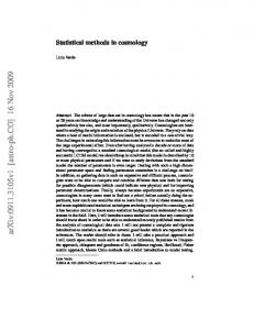
Figure 2. Comparison of MAK reconstructed and analytical ellipticity distribution – We represent here the distribution of ellipticity of the voids, marginalised over all possible SΨ . We used black squares for the ellipticity distribution obtained using the MAK reconstructed displacement field applied on the simulation. The dashed blue curve is computed using the unconditional Doroshkevich (1970) formula. The red curve is our new formula obtained by conditioning that voids are regions where the density field has a positive curvature. The left panel gives the result for all voids (true, pancake and filament). The right panel gives the result for only true voids. The blue dashed curve and red solid curve overlap. All fields were smoothed with a Gaussian kernel of radius 4h−1 Mpc.

cosmology. This indicates that the two curvatures are quite strongly linked. Thus, enforcing that Tl,m is positive causes the curvature of SΨ to be preferentially negative. So, the two distributions of the right panel of Fig. 2 should be similar. On the other hand, for the left panel no such implication exists, which leads to the largely evident discrepancies of ellipticities. We note the distributions of the right panel are only measurable using our void finder as the other ones cannot distinguish truly expanding voids and pancake voids just by looking at their shape. Number of voids – Now that we know the shape the voids should have in the context of linear theory, we would like to know how many of them should be present in the Universe. With our definition of voids, we may conveniently use the results obtained by Bardeen et al. (1986) for Gaussian random fields. In particular in the equation (4.11b), they show that the average number density of maxima is equal to √ 29 − 6 6 ≃ 0.016R∗−3 . (31) nmax = 3/2 5 2(2π)2 R∗3 with R∗ =

r

3

S4 S6

(32)

in our notation. We note that this is a mean number, so we expect some fluctuation according to the mean which are difficult to compute analytically. Tests on Gaussian random field seems to point out that the number of voids are distributed like a Poisson distribution. We also expect this number to slightly overestimate the actual density of voids that we will find in simulations (Section 5.2).

In the next section, we are now going to confront the analytical model with the results given by DIVA applied on N -body simulations.

5

TEST ON N -BODY SIMULATIONS

In this section, we are going to identify voids in the N -body samples described in Section 5.1. We then give a sketch (Section 5.2) of the procedure we followed to perform the MAK reconstruction, which corresponds to the one described in Lavaux et al. (2008). In Section 5.3, we focus on the results obtained at z = 0. First, we give an illustration of a void of each class in Section 5.3.1. We then compare the results obtained using the displacement field given by the simulation and the one reconstructed by MAK (Section 5.3.2). There, we also detail the number of voids detected and their ellipticities for both fields. We compare quantitatively the distribution of Eulerian volume ellipticity to the Lagrangian tidal ellipticity in Section 5.3.3. Finally, we check the validity of the analytical model on the simulated displacement field (Section 5.3.4). In Section 5.4, we look at the evolution of the mean ellipticity for a simulation with w = −1 and in the analytical model. At last, in Section 5.5, we assess the possibility of measuring the evolution of the mean ellipticity in two simulations where w is either −1 or −0.5. 5.1

The N -body simulations

To test our void finder, we use three large volume N -body simulations but with medium resolution of N = 5123 , L =

8


500h−1 Mpc, Ωm = 0.30, ΩΛ = 0.70, H = 65 km s−1 Mpc−1 , ns = 1, σ8 = 0.77, Ωb = 0.04. The N -body simulations contains only dark matter and we include the effect of baryons only through power spectrum features in the initial conditions. This essentially reduces power on scales smaller than the sound horizon and introduces Baryonic Acoustic Oscillations. The two first N -body simulation (ΛSIM and ΛSIM2) corresponds to a standard ΛCDM cosmology for which the equation of state is given by w = −1. ΛSIM and ΛSIM2 have exactly the same cosmology but have different initial conditions. They will allow us to assess the impact of looking at two different realisations of the initial conditions. The third, wSIM, is assuming an equation of state w = −0.5 for the Dark Energy. To build the initial conditions, we modified the GRAFIC (Bertschinger 2001) package to use the power spectrum generated by the CAMB package (Lewis et al. 2000). We reach a sub-Mpc resolution scale which is sufficient for proper description of most voids (1-20 h−1 Mpc). The intermediately large volume allows accounting for large-scale tidal field effects and cosmic variance effects. We used the parallelised version of the RAMSES N -body code (Teyssier 2002) and run it both on the Cobalt NCSA supercluster and the Teragrid NCSA supercluster through Teragrid facilities (Catlett et al. 2008). We modified RAMSES to simulate cosmologies with a dark energy equation of state different than w = −1. To account for the impact of clustering, we analyse the displacement field for which the mass of dark matter halos has been put to the centre of mass of these halos. To be able to do that, we construct a halo catalogue using a Friend-ofFriend algorithm with a traditional linking value of l = 0.2 (Davis et al. 1985; Efstathiou et al. 1988). We put a threshold of Np = 8. This prescription in practice should mostly erase the information contained in halos while retaining the dynamics outside of them. Though the use of such a low number for the particles of halos are questionable for the study of the properties of those halos, we are not here interested in them. We are only interested in checking that we keep most of the information useful to study voids and their overall dynamics, even though we destroy the small scale information. The above prescription has already been successfully applied for the study of peculiar velocities with MAK (Lavaux et al. 2008). We note that we will only use the halo catalogue to do the MAK reconstruction. All the tests of the displacement field of the simulation are run on the particles of the simulation. We note that that the initial conditions of the simulation present two particularities that must be taken into account. The largest mode of the simulation box is klow = 1.25 × 10−2 h Mpc−1 thus introducing a sharp low-k cut. Additionally GRAFIC applies a Hanning filter on the initial conditions to avoid aliasing. In practice, GRAFIC multiplies the cosmological power spectrum by the following filter: Whanning (k) =

cos 0

1 k∆x 2

if k∆x 6 π , elsewhere

(33)

with ∆x = 0.976h−1 Mpc the Lagrangian grid step size of our simulations. These two features must be introduced in the power spectrum of Eq. (27) and (30) to make correct predictions for the simulation. In real observational data, no such features should be present.

5.2

MAK reconstruction and void identification

Among the different tests that we are going to present in the following, we have run only one MAK reconstruction for the full halo catalogue. We chose a resolution of 2563 mesh elements generated following the algorithm of Lavaux et al. (2008). This algorithm consists in splitting a mass in an integer number of MAK mesh elements, with the constraints that the splitting must be fair and the number of mesh elements is fixed and equal to 2563 . This method works well and has, so far, not been prone to biases. Choosing this number of elements gives us a resolution of ∼2h−1 Mpc on the Lagrangian coordinates of the displacement field. We cannot run it at the full simulation resolution due to the high CPU-time cost which hinders doing several reconstruction. One reconstruction takes ∼13,000 accumulated CPU-hours on Teragrid cluster at NCSA. However, as the complexity grows as O(N 2.25 ), increasing the resolution to 5123 would have consumed ∼ 106 CPU-hours. So we limited ourself on running the reconstruction at the 2563 resolution, the expected worst case for the performance of MAK. At higher redshift, the MAK reconstruction converges faster and gives a more and more precise displacement field compared to the one given by simulation. These two features are both caused by the decrease of small scale non-linearities at earlier times. We took the halo catalogue built on ΛSIM at z = 0 and ran a reconstruction on it. The other results presented in this paper use the displacement field given directly by the simulation after having checked that the reconstruction is indeed sufficient for our purpose. This is the case as we will not look at voids smaller than ∼1h−1 Mpc scale in Lagrangian coordinates. We chose two different smoothing scales on which we study the displacement field for voids: 2.5h−1 Mpc and 4h−1 Mpc. Once the displacement field has been smoothed, we compute the eigenvalues and the divergences in Fourier space. We then locate the maxima in the divergence of the displacement field. At each maxima, we compute the ellipticity ε with the help of Eq. (13), where the λi are taken as the eigenvalues of Tl,m (q). The displacement shear tensor, is computed numerically from Ψ(q) in Fourier space: Z 1 ˆ l (k)eik·q , Tl,m (q) = d3 kikm Ψ (34) (2π)3 k ˆ l (k) is the Fourier transform of the displacement where Ψ field in Lagrangian coordinates. All these quantities were evaluated using Fast Fourier Transform on the Lagrangian grid. In summary, the steps are the following: - First, we prepare a catalogue for a MAK reconstruction. This involves doing fair equal mass-splitting of the objects. - Next, we run the MAK reconstruction. - After the reconstruction is finished, we put the computed displacement field given by MAK on the homogeneous Lagrangian grid. - We smooth this displacement field and compute the tidal field Ti,j in Lagrangian coordinates in Fourier space using Eq.(34). - Now we compute SΨ (q) on the grid using Eq. (5), which corresponds to summing the three eigenvalues of Ti,j . - We look for local maxima in SΨ (q) using an iterative

Precision cosmology with voids: definition, methods, dynamics steepest descent algorithm. This gives us the list of the voids in Lagrangian coordinates. - Using these coordinates, we now compute the ellipticity using the eigenvalues of Ti,j at the location of the minima. - For computing the void boundary, we execute the modified Watershed transform of Section 3.1. This identifies the Lagrangian domain of the voids. The boundary of this domain is then transported using the displacement field to recover the Eulerian void volume. We now look at the results obtained with MAK, the simulation and the analytical model at z = 0 in the next section. 5.3 5.3.1

Results at z = 0 Example of found voids

Before going to the statistical study of the local shape εDIVA properties of void found by DIVA, we look at a visual example of each of the void type. We chose a filtering scale of 4h−1 Mpc in Lagrangian coordinates. We selected one void of each class. These three voids have the following properties: - The first void is a true void. The eigenvalues of the tidal field Tl,m (q) (8) at the centre are (1.2, 0.84, 0.69) along the three axis. We thus derive the ellipticity ε = 0.13. The volume of the void, in Lagrangian coordinates, is VL = 75240h−3 Mpc3 , which corresponds to an equivalent spherical volume given by a sphere of radius Requiv = (3/(4π) ∗ V )1/3 = 26h−1 Mpc. - The second void is a pancake void. The eigenvalues of the tidal field are (1.1, 0.11, −0.60), the ellipticity is 0.563 and the Lagrangian volume is VL = 1560h−3 Mpc3 , with Requiv = 7.2h−1 Mpc. - The last void is a filament void. Again, the eigenvalues of the tidal field are (0.99, −0.24, −0.61), the ellipticity is ε = 0.557 and the Lagrangian volume is VL = 260h−3 Mpc3 , with Requiv = 4.0h−1 Mpc. Those three voids are represented in three dimensions, along with the particles of the simulation in the same region, in Fig. 3. We note that the true voids is the largest one. We expect to observe that effect as true voids expands in three directions and thus are more likely to be bigger than pancake voids and filament voids. For these three cases, the surface delimited by DIVA seems to nicely fit to the structures located on the boundaries. In the case of the pancake and filament voids, we note that the cavity seem to be split into two pieces. This splitting is due to the Watershed transform criterion which isolated two void cavities separated by a structure. 5.3.2

MAK vs Simulation

We now concentrate on the properties of the voids at z = 0. This is the time where the density is the most non-linear and the reconstruction is the most difficult and therefore represents a worst case example. We take the displacement field given by the simulation as the field of reference to study voids. Indeed, this field has been obtained by solving completely the equation of motion for each particle. In this section, we will first compare the properties of the voids found using this field and the MAK reconstructed field. Then, we will focus on how it compares to the analytic model.

9

Filter

Predicted average number

Displacement field

Number of candidates

2.5h−1 Mpc

42908

4h−1 Mpc

11706

Simulated Reconstructed Simulated Reconstructed

31002 28397 10643 9412

Table 1. Unconditioned number of voids in ΛSIM – we give here the unconditioned number of voids found within the volume of the simulation, (500 h−1 Mpc)3 . The predictions are obtained using Equation (31) applied on the power spectrum of primordial density fluctuations multiplied by the Fourier transform of the indicated filter in the first column. The last column gives the actual number of void candidates that we found using the displacement field.

We represent on Fig. 4 the distribution of ellipticities obtained using both the reconstructed and the simulated displacement field. We also give the number of voids found in simulated displacement field, in the reconstructed displacement field and the expected number of maxima according to Eq. (31) (Table 1). To allow for a void-by-void comparison, we tried to match the voids found using the two displacement fields. We considered that two voids are the same if the distance between the two voids is less than a Lagrangian grid √ cell (d 6 3 lcell , with lcell the length of the side of a cell). At 2.5h−1 Mpc smoothing, the agreement of the ellipticity distribution derived from the simulated displacement and the MAK reconstructed displacement is very good, though the high ellipticity tail seems a little different in the two cases. This is actually due to a selection effect which, unfortunately, is correlated with the ellipticity. If we look at the number of voids detected using the two fields (Table 1), we see that MAK is missing about 10% of the voids detected in the simulation. The distribution of ellipticity of those voids happens to be skewed towards higher ellipticities. Thus it seems that we tend to miss the most elliptical voids. This behaviour is expected as these voids tend to be pancake voids. So they are closing along one direction, and the more elliptical they are the faster they are closing. If they close, the particles of these voids shell cross and MAK is not able to reconstruct the displacement field. Looking at this same distribution, but for a 4h−1 Mpc smoothing, we now barely see a difference between the two curves. We indeed checked that the ellipticity distribution of the voids that have not been identified using the MAK reconstructed displacement field is similar to the distribution of the other voids. The number of voids detected in the simulation looks less than the expected average number of minima (Table 1). This is also due to the destruction of minima by the collapse of large scale structures. When we look at the beginning of the simulation we find 11,485 minima (for Rf = 4h−1 Mpc), and this number steadily decreases to the value we put in the table as the simulation evolves. We estimated the mean and the variance in the number of minima using 20 realisations of a Gaussian random field with the same cosmology as the simulation. We found that the mean should be 11,762 and the standard deviation is 58, which is in agreement with the result given by the analytic computation. Using the match between voids coming from the two

10


Figure 3. Example of voids – We illustrate here the voids that are found using DIVA. Each of these belong to one of the void class that we listed in Section 3.1. The scale of the box is the same for the three cases: the side corresponds to 50h−1 Mpc.

fields, we can build a statistical error model in the form of the joint probability distribution P (εMAK , εSIM ) of getting an ellipticity εMAK using MAK displacement and an ellipticity εSIM ) using simulated displacement. It is important to check P (εMAK , εSIM ) if, as we will do in future, we want to estimate cosmological parameters from ellipticity distribution. This function tells us what accuracy we may expect on the ellipticity measurements. We represent this probability in the left panel of Figure 5. We see a strong correlation, already seen in Fig. 4, indicating a high accurate reconstruction. We also see that the error seems low. We represent at the left side of the thick red solid line of the right panel the conditional probability P (εMAK |εSIM ) that we computed us-

ing:

P (εMAK |εSIM ) = R 1

P (εMAK , εSIM ) P (ε, εSIM )dε =0

(35)

εMAK

wherever it was possible to evaluate the denominator. This conditional probability is mostly Gaussian, so we tried to estimate the standard error by computing the mean variance of the error on the ellipticity for the distribution between the two dotted red line εSIM ∈ [εS,min ; εS,max ] with εS,min =


11

Figure 4. MAK reconstructed ellipticity distribution vs. ellipticity distribution from simulated displacement field – This figure gives the ellipticity distribution computed using either the MAK reconstructed displacement field (solid black line) or the simulated displacement field (solid thick gray line). We represent the dispersion expected if the error on estimating the distribution come from the number of voids in a given bin. We assumed a Poisson distribution for the estimation of the error bar. The displacement fields were both smoothed with a Gaussian kernel of radius Rf = 2.5h−1 Mpc in the left panel and to Rf = 4h−1 Mpc in the right panel.

Figure 5. Ellipticity derived from the simulated displacement field vs. the MAK displacement field – We represent here a scatter plot between the ellipticities of the voids that were both detected in the MAK reconstructed displacement field and the simulated displacement field, both smoothed at 4h−1 Mpc. In the left panel, we show the raw joint probability distribution of the two ellipticities. The gray-scale is linear in the density of probability. In the right panel, we represent the conditional distribution of εMAK given εSIM , on the left of the thick vertical line. On the right of this same line, we represent this same distribution if one uses the estimated standard deviation σε of the error. It is estimated using the distribution between the two vertical dotted lines. The estimated standard deviation is σε = 0.018.


12

1.0

been used so far, seems thus to be a poor proxy of the tidal ellipticity, which we manage to recover with extreme precision using our Lagrangian orbit reconstruction technique. For the rest of this paper, we will only use the tidal ellipticity.

0.8

5.3.4 εvol

0.6

0.4

0.2

0.0 0.0

0.2

0.4

0.6

0.8

1.0

εDIVA Figure 6. Tidal ellipticities vs Volume ellipticity – This plot gives a comparison of the ellipticity of the void as determined either using the shear of the displacement field [εDIVA , Eq. (13)] or using the overall shape of the void [εvol , Eq. (15)].

0.15 and εS,max = 0.40. With this notation, we computed 1 εS,max − εS,min sZ Z εS,max 1 dε

σε =

ε=εS,min

εmak =0

dεmak (εmak − ε)2 P (εmak |ε).

(36)

Within the interval limited by the two dotted red line, we estimate σε ≃ 0.018. At the right of the vertical red solid line, we show the function P (ε|εSIMU , σε ) = √

− 1 (ε−εSIMU )2 1 e 2σε2 2πσε

(37)

with σε as estimated above. We note that this model of the conditional probability (right of the vertical solid line) looks much like the actual ellipticity discrepancy (left of the vertical solid line).

5.3.3

Simulation vs Analytic

In this section, we compare the results obtained on the simulated displacement field and the prediction given by the analytical model of Section 4. We represented in the left panel of Fig. 2 the ellipticity distribution of all observable voids as defined in Section 3.1. The black points give the ellipticity distribution for voids in the reconstructed displacement field. We estimated error bars assuming a Poisson distribution of the number of voids in each bin. The red line is obtained using the method of Appendix B. The dashed blue line is obtained through the formula of Park & Lee (2007), where no constraints are put on the curvature of the density field where the ellipticity of the void is measured. The success of the comparison between the black points and the solid red curve is striking. It shows the importance of our constraint that we only look in the negatively curved part of SΨ . We note that this should be a robust feature for voids found with any void finder. Any probe of the ellipticity in voids looks in regions of the density field that is strongly underdense, and thus should come mainly from initially underdense regions. In these primordial underdense regions, the curvature of the density field is likely to be positive, which corresponds to a negatively curved SΨ in our case. Our measured ellipticity distribution in the simulation is very clean because we rely on features of the displacement field which can be understood in terms of linear theory even at redshift z = 0. In the right panel of Fig. 2, we show this same ellipticity distribution but only for “true voids”. The comparison between simulation and analytic is also here successful. As we noted in Section 4.3, there is no real difference between the two models in this case. However, there is no way a purely geometrical analysis could yield this curve from the observation of galaxy catalogues, as this requires the knowledge of the sign of eigenvalues of Tl,m (Eq. 6). We note a small shift of ∼1-3% between the model and the reconstruction. We find, using numerical experiments with Gaussian random fields, that a fraction of this shift may be explained by the finite bin size and the very strong steepness of the distribution represented in this panel.

Volume ellipticity εvol vs. Tidal ellipticity εDIVA

In Fig. 6, we represented a comparison between the ellipticity of the volume, εvol , and the local tidal ellipticity, εDIVA . The volume ellipticity is computed using the Eq. (15), with the inertial mass tensor M as computed using the smoothed displacement field. Visually, the two variables seem loosely correlated. We observe they do follow each other but this correlation just get worse when the ellipticity increases. This is expected as the volume ellipticity is a non-local quantity and thus is sensitive to all local ellipticities in the void volume. This is what makes εvol more difficult to use as a precise cosmology probe. We show in Appendix C that these two quantities are indeed related but only to first order. This explains that the scatter seems smaller for small ellipticities than for high ellipticities. The volume ellipticity, which has

5.4

Evolution with redshift

In this section, we focus on the evolution with redshift of the ellipticity of voids. This evolution has been shown to be analytically a sensitive probe of w by Lee & Park (2009). We took snapshots of the simulation at different redshifts and computed the ellipticity distribution in each of these snapshots. We note that we must at least have two main differences compared to what would happen with observations. First, we may have a systematic effect in the evolution of the mean ellipticity as we are studying only a single realisation of initial conditions. Second, the number of available voids should be a non-trivial function of redshift. Second, because of both volume and selection effects, the error bars should


13

Figure 7. Evolution of the mean ellipticity with redshift – We represent the evolution of the mean ellipticity with redshift for the two ΛCDM simulations (left panel) and the wCDM simulation (right panel). The mean ellipticities deduced from ΛSIM are represented using square symbols, and the ones from ΛSIM2 using triangular symbols. The solid curve is obtained using the statistical model of Appendix B and changing σ8 according to the growth factor as specified in Eq. (38). The bottom panels give the relative difference, in percentage, between the simulation and the analytical model. In the bottom left panel, the points at ∼2% correspond to the square symbols

be large at both small and large redshift, while attaining a minimum at some intermediate redshifts The exact numbers for this second problem depends on the specific considered galaxy survey, in particular the apparent magnitude limit and the incompleteness function. To compute the predicted ellipticity distribution at any given redshift z, we simply scale the σ8 (z) parameter using the growth factor D(z):

tained from the simulated displacement field. This gives an interval on which the mean ellipticity can be trusted.

with P (ε|z) the probability distribution of the ellipticity ε at redshift z. The red solid line gives the prediction given by the analytic model of Section 4. The black points are obtained from the simulated field. The error bar on the mean ellipticity is estimated using σε σε¯ ≃ √ (40) Nvoids

In the left panel of Fig. 7, we see that the agreement between the analytical model and the one from the simulated displacement field (square symbols, “Simulation 1”) is very good for w = −1. Looking at the relative error between the model (lower-left panel) and the simulation yields a systematic ∼2% deviation relative to the expectation. The main reason is the inexactness of the initial conditions to the finite number of modes available in the simulation box. Even though the power spectrum is normalised to σ8 = 0.77, the realized σ8 of the displacement field is 0.783. This produces intrinsically a shift of 1.7% towards positive errors. It is exactly what we observe. As we see, this bias is relatively modest. However it should be observable when we look the small amplitude of the expected reconstruction errors given by the small error bars. To check this effect, we rerun another simulation with the exact same cosmology but with another seed. This time, we measured σ8 = 0.7688 in the initial conditions, this corresponds to a small statistical fluctuation of −0.15%. We plotted the corresponding evolution of the mean ellipticity in the left panel of Fig. 7 (triangular symbols, “Simulation 2”).

with σε = 0.02 as estimated in Section 5.3.2 for a smoothing scale of 4h−1 Mpc. For Nvoids ≃ 104 , this gives a typical error of σε¯ = 2 × 10−4 on the mean. This error bar corresponds to the uncertainty of the ellipticity derived from the MAK reconstructed displacement field with respect to the one ob-

This will not prevent applying this method to observations for two reasons. First, we will marginalise over the bias and so the systematic shift will disappear. Second, each considered slice should be a nearly independent random realisation of a Gaussian random field normalised to the same

σ8 (z) = σ8 (z = 0) ×

D(z) . D(z = 0)

(38)

For clarity we only represent on Fig. 7 the mean ellipticity ε¯, defined as, Z 1 ε¯(z) = εP (ε|z)dε (39) 0

14

G. Lavaux & B. D. Wandelt 0.26

σ8 . Thus the points should be scattered according to our dashed horizontal line “0%” and not systematically pushed up or down.

Model w=−1 Model w=−0.5 Simulation 2 w=−1 Simulation w=−0.5

0.24

w = −0.5 vs w = −1.0

In all the previous sections, we studied the case of a standard ΛCDM cosmology with w = −1. However, we first started to look at voids to check if they may be good tracers of the properties of the dark energy, and in particular of the growth factor. We now focus on the results obtained from wSIM, a wCDM simulation with w = −0.5 as we specified in Section 5.1. The results are presented in the right panel of Fig. 7 and in Fig. 8. We computed that our particular realisation of the initial conditions had σ8 = 0.773, which is 0.33% above 0.77. We again note that the discrepancy in the lower-right panel in Fig. 8 has the correct systematic shift at low redshift. Taking into account this shift, as previously, the analytical model seems to follow the results given by simulation at the 0.1% level, taking into account the statistical uncertainty. The points obtained from the simulation are in excellent agreement with the simulation. Current redshift galaxy catalogues map the Universe at intermediate redshifts 0 . z . 1. We check if our method is sufficiently sensitive to distinguish a w = −0.5 from a w = −1 cosmology in Figure 8. In this figure, we used the σ8 as measured in the simulations to compute the analytical predictions (red and blue solid curves). We note that even at z ≃ 0.2, the behaviour of the two curves is already significantly different and above statistical uncertainties. If we consider the whole interval between z = 0 and z = 1, the difference is very significant compared to the uncertainties, with an ellipticity that changes by ≃35%. In all the above we considered catalogues with an important observable number of voids (typically ∼10,000). We do not expect to have such a high number available in catalogues. Now we try to make an estimate of the error bars on the mean ellipticity that we may expect. The SDSS covers one fifth of the sky. We now limit the survey at z = 0.1 (∼300h−1 Mpc), and we take a Lagrangian smoothing scale of 5h−1 Mpc. This smoothing scale is motivated by the average density of galaxies in the SDSS, which in band r is about 1 − 5 × 10−2 h3 Mpc3 (Blanton et al. 2003). This gives a mean separation of ∼ 2 − 4h−1 Mpc. The equation (31) predicts that we should observe ∼1,000 of our voids in this volume when smoothing the density field in Lagrangian coordinates with a Gaussian of radius 5h−1 Mpc, taking into account the survey coverage. If we go to z = 0.2, this number should increase to ∼9,000. This means that the error bars should only be moderately larger than the one that we considered in this work. Typically we expect about three times larger. Even, with this amount of uncertainty, the comparison to the analytic model should be able to highly constrain the equation of state of dark energy at z . 0.2. The Fisher matrix analysis is done in a companion paper.

6

COMPARISON OF DIVA TO EARLIER VOID FINDERS

In this section, we discuss how our technique is related to the other existing void finders. We try to make a qualitative

(z)

5.5

0.22

0.20

0.18

0.0

0.5

1.0

Redshift (z) Figure 8. Difference between w=-1 and w=-0.5 – We plotted here the evolution of the mean ellipticity with redshift. We used the simulation ΛSIM2 (square) and wSIM (triangle). The red solid line gives the prediction for σ8 = 0.7688, w = −1. The blue solid line gives the prediction σ8 = 0.773 and w = −0.5. These two values of σ8 have been computed using the initial conditions of the two simulations.

assessment of its strengths and weaknesses compared to the three classes of void finders define in Section 1. The void finders of the first class try to find emptier regions in a distribution of points, which in actual catalogues correspond to galaxies. The void finder developed by El-Ad et al. (1997), and one of its later versions by Hoyle & Vogeley (2002), is popularly used in observations (Hoyle & Vogeley 2004; Hoyle et al. 2005; Tikhonov & Karachentsev 2006; Foster & Nelson 2009). In these void finders, the first step consists in classifying galaxies in two types. Galaxies may lie in a strongly overdense region, in this case we consider it as a “wall galaxy”. The other possibility is that they lie in a mildly underdense region, and they are then called “field galaxies”. The exact separation between “wall galaxies” and “field galaxies” depends on an ad-hoc parameter. This parameter specifies how the local density of galaxy control the type (field or wall) of the galaxy. The voids are then grown from regions empty of wall galaxies. This classification thus gives a non-trivial dependence of the void sizes and shapes on the galaxy bias and catalogue selection function. Additionally, this definition depends on an ad-hoc empirical factor. These issues make the quantitative study of the geometry of voids difficult, while they find voids that correspond to the visual impression given by large scale structures in redshift catalogues of galaxies. Void finders belonging to the second class look for particularities in the continuous three dimensional distribution of the dark matter traced by galaxies. Of course, from observational data, one has then to first project and then smooth the distribution of galaxies to obtain this distribution. Different techniques are used:

Precision cosmology with voids: definition, methods, dynamics - One technique is to adaptively smooth the galaxy distribution either using an SPH technique (see e.g. Colombi et al. 2007) or a Delaunay Tesselation Field Estimator (Schaap & van de Weygaert 2000). Voids must then be identified from the smooth distribution derived using either of these techniques. One option is to use a scheme similar to El-Ad et al. (1997) or Hoyle & Vogeley (2002) to identify shapes of underdensity in the vicinity of a minima of the density field (Colberg et al. 2005). As with void finders of the first class, the galaxy bias does not affect the positions of the voids but their overall properties. A second option is to use a Watershed Transform (Platen et al. 2007) to identify the cavities of the voids. In this case, the galaxy bias does not affect the structure of the cavities. However, devising an efficient way of relating the geometrical properties of these cavities to the cosmology, which corresponds to studying Morse theory, could well be non-trivial (Jost 2008). Some work to study the skeleton (also called the “cosmic spine”) of Large Scale structures in this theory has been recently done by Aragon-Calvo et al. (2008), Pogosyan et al. (2009) and Sousbie et al. (2009). - A second technique consists in using the local density estimated using the Voronoi diagram of a Delaunay tessellation to locate minima (Neyrinck 2008). The particles are first grouped in zones. Each particle is assigned to a zone on to where this particle is attracted if it followed the density gradient as in the watershed technique. Each zone is defined to be a void. But it is also possible to define a hierarchy of voids by checking, for two neighbouring voids, which of the two has the lowest density at the minima. The zones are then grouped and a probability of being a void is assigned depending on the contrast between the density at the ridge of the void and its depth. This void finder has the advantage of defining voids in terms of topology of the density field, which is easier to handle from a theoretical point of view and may better define a void in terms of dark matter. Still, we are faced with the task of relating the shape of the voids that are found by these algorithms, which is non-local by nature, to cosmology. As mentioned previously for void finders of the first class, this seems to be non-trivial. Void finders of the third class use the inferred dark matter distribution but they do a dynamical analysis to infer the location of these voids. DIVA belongs to these class of void finders. There are two advantages of looking at dynamics for voids. (i) It gives a much more physical and intuitive definition of these structures: voids corresponds to places in the universe from which the matter is really escaping and not gravitationally unstable at present time. (ii) Using this criterion, one is bound to use either the velocity field or the displacement field. These two quantities are highly linear. It has been directly shown for velocity fields by Ciecielg et al. (2003) and indirectly shown by Mohayaee et al. (2006) and Lavaux et al. (2008) for the displacement field. This linearity helps us at constructing an analytical statistical model of the voids. Hahn et al. (2007) and Forero-Romero et al. (2009) attempted to classify structures according to a criterion on the gravitational field. However we may highlight two very important differences compared to the approach we are following here: - we are using a purely Lagrangian method and it takes

15

into account the true evolution of the void and not how virtual tracers in the void should move now, - we put an exact natural threshold on eigenvalues to classify voids. This is in contrast with Forero-Romero et al. (2009) where they need to to put a threshold on eigenvalues depending on an estimated collapse time. In our case, everything is already integrated in the definition of the displacement field. Moreover, the Monge-Ampère-Kantorovitch reconstruction presents the two advantages of: (i) never diverging in the neighbourhood of large density fluctuations, compared to a pure gravitational approach, (ii) recovering exactly the Zel’dovich approximation in the neighbourhood of centres of voids. As for the other void finders, DIVA depends on galaxy bias. We recall that the bias b is defined with δg ≃ bδm ,

(41)

with δg the density fluctuations of galaxies and δm the density fluctuations of matter. As MAK is essentially reconstructing the Zel’dovich displacement in underdense regions, and that the Zel’dovich potential is proportional to density fluctuations, the MAK displacement should also be mostly linear with the bias. We describe in a second paper (Lavaux & Wandelt 2009, in prep.) how to relate the volume of the voids that we find in Lagrangian coordinates to the voids that we observe in Eulerian coordinates.

7

CONCLUSION

We have described a new technique to identify and characterise voids in Large Scale structures. Using the MAK reconstruction, we have been able to define void centres in Lagrangian coordinates by assimilated them to the maxima of the divergence SΨ of the displacement field, interpreted as its source term. The scalar field SΨ has the interesting property of being nearly equal to the opposite of the linearly extrapolated primordial density field (Mohayaee et al. 2006). This allowed us to consider that the statistics of those two fields were equal. Using that, we made predictions on the number of voids in Lagrangian coordinates, along with their ellipticities defined using the eigenvalues of the curvature of SΨ . We tested our model using N -body simulations with different cosmologies (w = −1 and w = −0.5). We checked, using the largest Lagrangian reconstruction run so far, that MAK is capable of recovering the ellipticity of individual voids to the order of a few percent. We highlighted the importance of using our model for the statistics of the eigenvalues of the curvature instead of the formula of Doroshkevich (1970) for the particular case of voids. We showed that our analytical model agrees within ∼0.1-0.3% to results obtained with MAK and the displacement field obtained from the simulation. We expect our method to be able to provide a very promising constraint on the equation of state of the Dark Energy of the late universe, especially given the notable accuracy of the prediction that we obtained Fig. 8. We intend to pursue this work to continue characterising analytically the voids found by DIVA, in particular

16


the evolution of the number of voids and their size distribution. We will make further robustness tests using mock catalogues, including especially redshift distortion effects. We also would like to apply our method to the Luminous Red Galaxy sample of the SDSS DR7 (Abazajian et al. 2009).

ACKNOWLEDGEMENTS This research was supported in part by the National Science Foundation through TeraGrid resources provided by the NCSA. TeraGrid systems are hosted by Indiana University, LONI, NCAR, NCSA, NICS, ORNL, PSC, Purdue University, SDSC, TACC and UC/ANL. The authors acknowledge financial support from NSF grant AST 07-08849. We acknowledge the hospitality of the California Institute of Technology, where the authors completed most of this work. We thank the referee, Rien van de Weygaert, for his useful comments and suggestions.

REFERENCES Abazajian K. N., Adelman-McCarthy J. K., Ag¨ ueros M. A., et al. 2009, ApJS, 182, 543 Aragon-Calvo M. A., Platen E., van de Weygaert R., Szalay A. S., 2008, ArXiv e-prints Bardeen J. M., Bond J. R., Kaiser N., Szalay A. S., 1986, ApJ, 304, 15 Benoist C., Maurogordato S., da Costa L. N., Cappi A., Schaeffer R., 1996, ApJ, 472, 452 Benson A. J., Hoyle F., Torres F., Vogeley M. S., 2003, MNRAS, 340, 160 Bertschinger E., 1983, ApJ, 268, 17 Bertschinger E., 1985, ApJS, 58, 1 Bertschinger E., 2001, ApJS, 137, 1 Bertsekas D. P., 1979, A Distributed Algorithm for the Assignment Problem. MIT Press, Cambridge, MA Blanton M. R., Hogg D. W., Bahcall N. A., Brinkmann al. 2003, ApJ, 592, 819 Blumenthal G. R., da Costa L. N., Goldwirth D. S., Lecar M., Piran T., 1992, ApJ, 388, 234 Bond J. R., Myers S. T., 1996, ApJS, 103, 1 Brenier Y., Frisch U., Hénon M., Loeper G., Matarrese S., Mohayaee R., Sobolevski˘i A., 2003, MNRAS, 346, 501 Catlett C., Hallcock W. E., Andrews P., Aydt R., al. 2008, in Lucio Grandinetti ed., HPC and Grids in Action Vol. 16 of Advances in Parallel Computing, TeraGrid: Analysis of Organization, System Architecture, and Middleware Enabling New Types of Applications. pp 225–249 Ciecielg P., Chodorowski M. J., Kiraga M., Strauss M. A., Kudlicki A., Bouchet F. R., 2003, MNRAS, 339, 641 Colberg J. M., Pearce F., Foster C., Platen E., al. 2008, MNRAS, 387, 933 Colberg J. M., Sheth R. K., Diaferio A., Gao L., Yoshida N., 2005, MNRAS, 360, 216 Colless M., Dalton G., Maddox S., Sutherland W., Norberg P., al. 2001, MNRAS, 328, 1039 Colombi S., Chodorowski M. J., Teyssier R., 2007, MNRAS, 375, 348 Croft R. A. C., Gaztanaga E., 1997, Mon. Not. Roy. Astron. Soc., 285, 793

Davis M., Efstathiou G., Frenk C. S., White S. D. M., 1985, ApJ, 292, 371 de Lapparent V., Geller M. J., Huchra J. P., 1986, ApJL, 302, L1 Doroshkevich A. G., 1970, Astrophysics, 6, 320 Efstathiou G., Frenk C. S., White S. D. M., Davis M., 1988, MNRAS, 235, 715 El-Ad H., Piran T., Dacosta L. N., 1997, MNRAS, 287, 790 Erdogdu P., Huchra J. P., Lahav O., et al. 2005, MNRAS Forero-Romero J. E., Hoffman Y., Gottl¨ ober S., Klypin A., Yepes G., 2009, MNRAS, 396, 1815 Foster C., Nelson L. A., 2009, ApJ, 699, 1252 Goldwirth D. S., da Costa L. N., van de Weygaert R., 1995, MNRAS, 275, 1185 Gottl¨ ober S., Lokas E. L., Klypin A., Hoffman Y., 2003, MNRAS, 344, 715 Gregory S. A., Thompson L. A., 1978, ApJ, 222, 784 Hahn O., Porciani C., Carollo C. M., Dekel A., 2007, MNRAS, 375, 489 Hausman M. A., Olson D. W., Roth B. D., 1983, ApJ, 270, 351 Hoffman G. L., Salpeter E. E., Wasserman I., 1983, ApJ, 268, 527 Hoffman Y., Shaham J., 1982, ApJL, 262, L23 Hoyle F., Rojas R. R., Vogeley M. S., Brinkmann J., 2005, ApJ, 620, 618 Hoyle F., Vogeley M. S., 2002, ApJ, 566, 641 Hoyle F., Vogeley M. S., 2004, ApJ, 607, 751 Huchra J. P., 2000, in Courteau S., Willick J., eds, Cosmic Flows Workshop Vol. 201 of Astronomical Society of the Pacific Conference Series, The 2MASS Redshift Survey. pp 96–+ Icke V., 1984, MNRAS, 206, 1P Joeveer M., Einasto J., Tago E., 1978, MNRAS, 185, 357 Jones D. H., Read M. A., Saunders W., et al. 2009, MNRAS, 399, 683 Jost J., 2008, Riemannian Geometry and Geometric Analysis. Universitext, Springer Berlin Heidelberg Kauffmann G., Fairall A. P., 1991, MNRAS, 248, 313 Kirshner R. P., Oemler Jr. A., Schechter P. L., Shectman S. A., 1981, ApJL, 248, L57 Lavaux G., Mohayaee R., Colombi S., Tully R. B., Bernardeau F., Silk J., 2008, MNRAS, 383, 1292 Lavaux G., Tully R. B., Mohayaee R., Colombi S., 2008, ArXiv e-prints Lee J., Park D., 2006, ApJ, 652, 1 Lee J., Park D., 2009, ApJL, 696, L10 Lewis A., Challinor A., Lasenby A., 2000, ApJ, 538, 473 Martel H., Wasserman I., 1990, ApJ, 348, 1 Mohayaee R., Mathis H., Colombi S., Silk J., 2006, MNRAS, 365, 939 Neyrinck M. C., 2008, MNRAS, 386, 2101 Norberg P., Baugh C. M., Hawkins E., al. 2001, MNRAS, 328, 64 Novikov D., Colombi S., Doré O., 2006, MNRAS, 366, 1201 Park D., Lee J., 2007, Physical Review Letters, 98, 081301+ Park D., Lee J., 2009a, MNRAS, pp 1323–+ Park D., Lee J., 2009b, MNRAS, 397, 2163 Patiri S. G., Betancort-Rijo J. E., Prada F., Klypin A., Gottl¨ ober S., 2006, MNRAS, 369, 335 Peebles P. J. E., 1989, ApJL, 344, L53

Precision cosmology with voids: definition, methods, dynamics Percival W. J., Nichol R. C., Eisenstein D. J., et al. 2007, ApJ, 657, 645 Piran T., Lecar M., Goldwirth D. S., da Costa L. N., Blumenthal G. R., 1993, MNRAS, 265, 681 Platen E., van de Weygaert R., Jones B. J. T., 2007, MNRAS, 380, 551 Platen E., van de Weygaert R., Jones B. J. T., 2008, MNRAS, 387, 128 Plionis M., Basilakos S., 2002, MNRAS, 330, 399 Pogosyan D., Pichon C., Gay C., Prunet S., Cardoso J. F., Sousbie T., Colombi S., 2009, MNRAS, pp 673–+ Regos E., Geller M. J., 1991, ApJ, 377, 14 Ryden B. S., 1995, ApJ, 452, 25 Ryden B. S., Melott A. L., 1996, ApJ, 470, 160 Sahni V., Sathyaprakah B. S., Shandarin S. F., 1994, ApJ, 431, 20 Sahni V., Shandarin S., 1996, MNRAS, 282, 641 Schaap W. E., van de Weygaert R., 2000, A&A, 363, L29 Shandarin S., Feldman H. A., Heitmann K., Habib S., 2006, MNRAS, 367, 1629 Sheth R. K., van de Weygaert R., 2004, MNRAS, 350, 517 Sousbie T., Colombi S., Pichon C., 2009, MNRAS, 393, 457 Tegmark M., Blanton M. R., Strauss M. A., al. 2004, ApJ, 606, 702 Tegmark M., Eisenstein D. J., Strauss M. A., Weinberg D. H., Blanton M. R., al. 2006, PhRvD, 74, 123507 Teyssier R., 2002, A&A, 385, 337 Tikhonov A. V., Karachentsev I. D., 2006, ApJ, 653, 969 Tully R. B., Fisher J. R., 1978, in Longair M. S., Einasto J., eds, Large Scale Structures in the Universe Vol. 79 of IAU Symposium, Nearby small groups of galaxies. pp 31–45 van de Weygaert R., van Kampen E., 1993, MNRAS, 263, 481 York D. G., Adelman J., Anderson Jr. J. E., Anderson S. F., Annis J., al. 2000, AJ, 120, 1579 Zel’dovich Y. B., 1970, A&A, 5, 84

the matrix V of the variances  3 1 1 0 0 0  1 3 1 0 0 0  σ2   1 1 3 0 0 0 V = 15   0 0 0 1 0 0  0 0 0 0 1 0 0 0 0 0 0 1

17

       

thus the covariance matrix C is  4 −1 −1  −1 4 −1  15  −1 −1 4 −1  C=V = 0 0 10σ 2   0  0 0 0 0 0 0

(A3)

0 0 0 10 0 0

0 0 0 0 10 0

0 0 0 0 0 10

       

(A4)

The unconditional probability dP ({TA }) of observing these components at a point in the universe is given by ! 6 6 Y 3375 1 X dP ({TA }|σ) = √ dTA CA,B TA TB exp − 6 3 2 A,B=1 16 5σ π A=1 (A5)

We want now to make a change of variables and get the probability distribution of the eigenvalues of Ti,j . The appendix B of Bardeen et al. (1986) shows that the infinitesimal volume is transformed according to: 6 Y

A=1

dTA = |(λ1 − λ2 )(λ1 − λ3 )(λ2 − λ3 )| dλ1 dλ2 dλ3 dΩS 3 , (A6)

with dΩS 3 the infinitesimal rotation of the hypersphere of dimension 3. The quadratic form Q in the argument of the exponential of Eq. (A5) may be expanded Q=

6 X

CA,B TA TB =

A,B=1

15 4(T12 + T22 + T32 ) σ2

−2(T1 T2 + T1 T3 + T2 T3 ) + T42 + T52 + T62 .

(A7)

Linear algebra tells us that the scalar quantities APPENDIX A: EIGENVALUES PROBABILITY DISTRIBUTION

K1 = T1 +T2 +T3 and K2 = T1 T2 +T2 T3 +T1 T3 −T42 −T52 −T62

In this appendix, we derive the unconditional distribution of the eigenvalues of the Jacobian matrix of the displacement field in the Zel’dovich regime. Starting from the potential Φ(q) of the displacement field at the comoving Lagrangian coordinate q, we define the Jacobian matrix of the displacement field

are invariant by change of vector basis. The quadratic form may then be rewritten: 6 5 Q = 2 K12 − K2 (A9) σ 2

Ti,j =

∂Φ . ∂qi ∂qj

(A1)

This matrix is real and symmetric. We assume the components to be normally distributed and to be as given by (Bardeen et al. 1986, Appendix A): hTi,j Tk,l i =

σ2 (δi,j δk,l + δi,k δj,l + δi,l δj,k ) , 15

(A2)

with σ the standard deviation of the density field. As it is a 3 × 3 real symmetric matrix, there are only 6 independent components. We label these components with A = 1 . . . 6, where each number refer to the (i, j) couples (1, 1), (2, 2), (3, 3), (1, 2), (1, 3) and (2, 3). We may now write

(A8)

We may now express K1 and K2 in terms of the eigenvalues:

K1

=

λ1 + λ2 + λ3 ,

(A10)

K2

=

λ1 λ3 + λ1 λ2 + λ2 λ3 .

(A11)

After integrating the expression (A5) over S 3 , we obtain the unconditional probability that the Jacobian matrix has the three ordered eigenvalues λ1 , λ2 and λ3 : P (λ1 , λ2 , λ3 |σ) = " # 3 2K12 − 5K2 3375 √ exp |(λ1 −λ2 )(λ1 −λ3 )(λ2 −λ3 )|. 2σ 2 8 5σ 6 π (A12) This equation corresponds to the distribution derived by Doroshkevich (1970).

18


APPENDIX B: PROBABILITY DISTRIBUTION OF TIDAL FIELD IN VOIDS We show in this Appendix how to compute the form of the probability distribution of the gravitational tidal field in the case of voids. The technique involved in this derivation looks much like the one used in Appendix A but with an extra complication due to correlations with the density field. By definition, void centres are chosen to be maxima of 3 X ∂2Φ SΨ (q) = . ∂qi2 i=1

(B1)

with Φ defined as in § 2, the scalar potential of the displacement field. We will assume that, for voids, we are fully in the Zel’dovich regime and thus we can equate Φ as given by MAK to the potential of the Zel’dovich displacement at high redshift. In this case, SΨ corresponds the primordial density fluctuations scaled linearly to z = 0. Being a maxima of SΨ means the displacement field satisfies two properties: the gradient of SΨ is null and the Hessian matrix Hi,j =

∂SΨ ∂qi ∂qj

(B2)

of SΨ is negative-definite. Thus our aim is to compute the probability of the Jacobian matrix of the displacement field given that Hi,j is symmetric negative-definite. We write this probability P (Ti,j |Hl,m < 0). We assume that the gravitational potential is a Gaussian random field determined by the power spectrum of matter density fluctuation P (k), with k a wave number. We compute the correlation between those two fields: hTi,j Tl,m i

=

σT2 (δi,j δl,m + δi,l δj,m + δi,m δj,l ) , 3

hHi,j Hl,m i

=

2 σH (δi,j δl,m + δi,l δj,m + δi,m δj,l ) , 3

hTi,j Hl,m i

=

ΓT H (δi,j δl,m + δi,l δj,m + δi,m δj,l ) , (B5) 3

(B3)

(B4)

with 2 σT2 = S2 = σ 2 and σH = S6 and ΓT H = −S4 ,

σ 2 the variance of the density field and Z +∞ 1 Sn = kn P (k)dk . 10π 2 k=0

(B6)

(B7)

A = 1 . . . 6, where each number refer to the (i, j) couples (1, 1), (2, 2), (3, 3), (1, 2), (1, 3) and (2, 3). The matrix V of the variance of the 12 reduced components may be formally written, using a block-matrix representation: A rA (B11) V = rA A and 

1 1 3 1 3

   A=  0   0 0

1 3

1 1 3

0 0 0

1 3 1 3

1 0 0 0

0 0 0 1 0 0

0 0 0 0 1 0

0 0 0 0 0 1



   .   

The inverse may be computed straightforwardly 1 A−1 −rA−1 C = M −1 = −rA−1 A−1 1 − r2

(B12)

(B13)

Now, we may express the joint probability P (T, H) of observing a tidal field T for the gravitational potential and a curvature H for the density field using the covariance matrix C = M −1 . p | det C| 1t P (T, H|r) = exp − Y CY (B14) (2π)6 2 with Y = (T, H). Now the probability of observing some matrix T given that H must be positive could be computed formally: Z P (T |r, H < 0) = P (T, H|r)dH (B15) H