Revised August 2004 SLAC-PUB-10371
Precision measurement of coupling ellipses parameters in a storage ring Y.T. Yan∗ and Y. Cai Stanford Linear Accelerator Center, Stanford, CA 94309
Abstract Eigen-mode coupling ellipses’ tilt angles and axis ratios can be precisely measured with a ModelIndependent Analysis (MIA) of the turn-by-turn BPM data from resonance excitation of the betatron motion. For each BPM location one can measure 4 parameters from the two resonance excitation, which completely describe the linear coupling of the location. Results from application to PEP-II LER storage rings are presented.
∗
Electronic address:
[email protected] Work Supported by the Department of Energy Contract DE-AC02-76SF00515
1
I.
INTRODUCTION
For an e+-e- collision, such as the PEP-II B-factory at the Stanford Linear Accelerator Center, a solenoid is usually imposed at the interaction point. This necessarily causes beam motion coupling between horizontal and vertical planes in each of the collision storage rings. To correct these coupling effect at IP and outside the solenoid region, designed lattice includes global skew and Local skew quadrupoles inserted at the suitable locations. However, during commissioning and operation, the linear coupling correction is not automatic; it usually requires dedicated effort of which precise measurement of the linear coupling is the key. Taking PEP-II Low-Energy Ring (LER) as an example, we show, in this paper, how we measure the linear coupling by measuring the eigen-mode coupling ellipses’ tilt angles and axis ratios to survey the linear couplings along an entire storage ring.
II.
HIGH-RESOLUTION TURN-BY-TURN ORBITS
The concept of coupling ellipses in a storage ring had been well known [1, 2]. Here we present a precision measurement technique with a simple model-independent analysis. To overcome the synchrotron radiation damping, We make two resonance excitations, one at the horizontal tune and the other at the vertical tune, for turn-by-turn BPM buffer data acquisition of about 2000 turns. Each excitation would allow for 2 sets of data stored in two matrices, one for the horizontal and the other for the vertical beam centroid readings. Columns of the matrices represent BPMs while rows represent the turns. For example, the PEP-II LER has 118 double-view BPMs and a total of 319 BPMs which can read 222 horizontal (X) and 215 vertical (Y) data per turn. Thus, for 2000 turn data acquisition, we would obtain, from each resonance excitation, a 2000-by-222 matrix for x readings and and a 2000-by-215 matrix for y readings. Excluding the closed-orbit mode, one can, through an automatical testing process, choose the right number of turns (< 1800 turns for 2000 turn data) such that making Fourier transformations on columns, one can match one and only one stand-out peak Fourier mode to the resonance frequency (tune) to obtain a cosinelike and a sine-like orbits from the mode for each of the excitation [3]. Therefore the two resonance excitations can offer a complete set of 4 clean betatron-motion orbits for one turn. Shown in Figure 1 is a typical set of 4 orbits for a given turn. To obtain the next turn
2
300
400
100
200
300
400
0
−2 0 2
100
200
300
400
0
−2 0
100 200 300 BPM sequence number
400
0
−2 0 1 Y2
200
100
200
300
400
100
200
300
400
100
200
300
400
0
−1 0 5 Y3
X2
100
0
−5 0 2 X3
Y1
0
−5 0 5
X4
2
0
−5 0 2 Y4
X1
5
0
−2 0
100 200 300 BPM sequence number
FIG. 1: Four High-resolution independent betatron motion orbits from measurement for PEP-II LER. The top two (blue) are from horizontal tune resonance excitation while the bottom two (red) are from vertical tune resonance excitation. (data acquired on September 30, 2003.)
orbits, one simply use the same number of turns for Fourier transformation but advance 1 turn for the block sub-matrix to be performed with the Fourier transformation. Repeat the process until one gets about 200 turns of the high resolution orbits. These consecutive-turn orbits from resonance excitations form two eigen-mode coupling ellipses at each double-view BPM location. Shown in Figure 2 are eigen-mode coupling ellipses at 4 double-view BPM locations, where, in each plot, the horizontal eigen-mode coupling ellipse is colored in blue while the vertical eigen-mode coupling ellipse is colored in red. Also shown in Figure 3 is a complete survey of the eigen-mode coupling ellipses for all but malfunction double-view 3
400
2
2 Plot 1
1 Y (mm)
Y (mm)
1 0 −1
0 −1
−2 −2
−1
0 x (mm)
1
−2 −2
2
2
−1
0 x (mm)
1
2
1
2
2 Plot 3
Plot 4
1 Y (mm)
1 Y (mm)
Plot 2
0
0
−1
−1 blue: Horizontal Eigen Ellipse
−2 −2
−2 −2
red: Verical Eigen Ellipse
−1
0 x (mm)
1
2
−1
0 x (mm)
FIG. 2: Eigen-mode coupling ellipses at 4 double-view BPM locations of the PEP-II LER. The top 2 are at the two BPMs beside the IP while the bottom 2 are at the tenth BPMs from IP in each side. (data acquired on September 30, 2003.)
BPMs in PEP-II LER.
III.
TILT ANGLE MEASUREMENT
For a horizontal eigen-mode coupling ellipse in the x-y plane, we define the tilt angle, αx as the counterclockwise angle of its long axis with respect to the x axis. If we make a counterclockwise rotation of the x-y axis for an angle that is equal to the tilt angle αx , then
4
FIG. 3: Eigen-mode coupling ellipses for all but malfunction double-view BPMs in PEP-II LER. The horizontal eigen-mode coupling ellipses are colored in blue while the vertical eigen-mode coupling ellipses are colored in red. Generally, a stronger coupling at a BPM location would result in a 5 larger tilt angle and a larger short-to-long axis ratio at the location. (data acquired on September 30, 2003.)
the ellipse long axis matches the new x axis, and the orbits’ new coordinates are given by x0i = xi cos αx + yi sin αx , yi0 = yi cos αx − xi sin αx . Considering a Least-Square fitting that the sum, D(αx ), of the distances of the ellipses’ orbits to the long axis be the minimum, one would have dD2 (αx )/dαx = 0, where D2 (αx ) = =
X
yi2 cos2 αx +
i
X
x2i sin2 αx −
i
X
X
2
y0i
i
xi yi sin 2αx ,
i
and so one obtains P xi yi 1 −1 2 αx = tan P 2i . 2 2 i (xi − yi )
(1)
By the same token, For a vertical eigen-mode coupling ellipse in the x-y plane, we define the tilt angle, αy as the counterclockwise angle of its long axis with respect to the y axis and obtain P xi yi 1 −1 2 . αy = − tan P 2i 2 2 i (yi − xi )
(2)
The tilt angles for the horizontal eigen-mode coupling ellipses shown in Figure 2 are respectively (12.0811o , 21.6461o , 25.9331o , −15.5012o ) for Plots 1-4. The corresponding vertical eigen-mode coupling ellipses tilt angles are (−3.8063o , 3.5516o , 28.3203o , −69.2074o ).
IV.
AXIS RATIOS MEASUREMENT
The horizontal eigen-mode coupling ellipse equation is given by x0 2 y 0 2 + 2 = 1, a2x ay where ax is the long axis and ay is short axis. Letting X 0 = x0 2 , Y 0 = y 0 2 , A = B=
1 , a2y
1 , a2x
and
one have a linear equation of AX 0 + BY 0 = 1,
6
(3)
which can be solved through Least-Square fitting of (Xi0 , Yi0 )s for the ratio of the short axis length over the long axis length given by (ay /ax ) =
p
A/B.
(4)
By the same token, one can get the axis ratio for the vertical eigen-mode coupling ellipse’s. Shown in figure 5 is the measurement of the eigen-mode coupling ellipse axis ratios at LER double-view BPM locations. The axis ratios for the horizontal eigen-mode coupling ellipses shown in Figure 2 are respectively (0.0630, 0.2867, 0.3560, 0.2494) for Plots 1-4. The corresponding vertical eigenmode coupling ellipses axis ratios are (0.0044, 0.0078, 0.1075, 0.4166).
V.
TILT ANGLE AND AXIS RATIO CALCULATION FROM ONE-TURN LIN-
EAR MAP
Let us first assume that the one-turn linear map, the 4-by-4 matrix M , has been decoupled and normalized as given by the following factorization [4], M = CARA−1 C −1 , where
cos µx sin µx
0
0
− sin µ cos µ 0 0 x x R= , 0 0 cos µ sin µ y y 0 0 − sin µy cos µy √
βx 0
0
0
−α 1 x √ √ 0 0 βx βx , p A= 0 0 βy 0 0 0 − √αy √1 βy
and
7
βy
C=
I cos φ
¯ sin φ W
−W sin φ I cos φ
where
W =
a b c d
,
¯ = −SW T S; and its conjugate W S=
0 1 −1 0
;I =
1 0 0 1
.
For horizontal eigen motion we have, in the eigen-mode plane at the nth -turn, √ cos nµx sin nµx x βx 0 = − sin nµx px − √αβxx √1βx n cosnµx cos µox sin µox A ox − sin µox cos µox 0 cos θx √ , = Aox βx 1 − βx (αx cos θx + sin θx )
(5)
where Aox is the resonance excitation normalized amplitude in the eigen space, and θx = nµx + µox . Transferring to the measurement (coupled) frame, at the nth -turn, we have x = Aox
p βx cos φ cos θx = Ax cos θx ,
which would yields cos θx = x/Ax and sin θx =
p
A2x − x2 /Ax ,
where Ax = Aox
8
p βx cos φ.
(6)
100 Tilt Angle (deg)
Horizontal Eigen Ellipses
50 0 −50
blue: ideal lattice red: measurement
−100
−1000
−500
0
500
1000
0 Distance from IP (meter)
500
1000
Tilt Angle (deg)
100 50
Vertical Eigen Ellipses
0 −50 −100
blue: ideal lattice red: measurement
−1000
−500
FIG. 4: Comparison of the PEP-II LER eigen-mode coupling ellipses tilt angles between measurement and the ideal lattice model. (data acquired on September 30, 2003.)
We would also have √ y = −Aox βx sin φ(a cos θx − = −Ax tanφ(a Axx −
b (αx βx
b (αx Axx βx
cos θx + sin θx ))
+
√ A−x2 −x2 ). Ax
We therefore get the ellipse equation as (Dx2 tan2 φ)x2 + 2[(a − where
bαx b2 )tanφ]xy + y 2 = A2x 2 tan2 φ, βx βx s
Dx =
(a − 9
bαx 2 b2 ) + . βx βx
1
Axis Ratios
0.8
blue: ideal lattice
Horizontal Eigen Ellipses
red: measurement
0.6 0.4 0.2 0
−1000
−500
0
500
1000
1
Axis Ratios
0.8
blue: ideal lattice
Vertical Eigen Ellipses
red: measurement
0.6 0.4 0.2 0
−1000
−500
0 Distance from IP (meter)
500
1000
FIG. 5: Comparison of the PEP-II LER eigen-mode coupling ellipses (short vs. long) axis ratios between measurement and the ideal lattice model. (data acquired on September 30, 2003.)
Counterclockwise rotating axis angle by ψx such that in the new coordinate frame, the x’y’ cross term disappear would yield x −2(a − bα )tanφ 1 βx ), ψx = tan−1 ( 2 1 − Dx2 tan2 φ
(7)
and the right ellipse equation would be given by Eq. 3 while the axis ratio given by Eq. 4,
10
Horizontal Eigen Ellipse
100 Tilt Angle (deg)
Tilt Angle (deg)
100 50 0 −50
Verical Eigen Ellipse
50 0 −50
blue: virtual machine
−100 red: measurement
−100
−1000 −500 0 500 1000 Distance from IP (meter)
−1000 −500 0 500 1000 Distance from IP (meter)
1
1 Horizontal Eigen Ellipse
0.8 Axis Ratios
Axis Ratios
0.8 0.6 0.4 0.2
Verical Eigen Ellipse
0.6 0.4 0.2
0 −1000 −500 0 500 1000 Distance from IP (meter)
0 −1000 −500 0 500 1000 Distance from IP (meter)
FIG. 6: Comparison of the PEP-II LER eigen-mode coupling ellipses’ tilt angles and (short vs. long) axis ratios between measurement and the virtual machine obtained through Green’s functions fitting [5]. (data acquired on September 30, 2003.)
where A and B are given by A=
cos2 ψx Dx2 tan2 φ + sin2 ψx + (a −
bαx ) sin 2ψx tanφ βx
2
A2x βb 2 tan2 φ
,
x
B=
sin
2
ψx Dx2 tan2 φ
2
+ cos ψx − (a −
bαx ) sin 2ψx tanφ βx
2
A2x βb 2 tan2 φ
.
x
By the same token one can calculate the tilt angle for the vertical eigen motion as y 2(d + bα )tanφ 1 βy −1 ), ψy = − tan ( 2 1 − Dy2 tan2 φ
11
where
s Dy =
(d +
bαy 2 b2 ) + 2. βy βy
The vertical eigen-mode coupling ellipse axis ratio (short axis over long axis) would be given by v u 2 u cos ψy Dy2 tan2 φ + sin2 ψy + (d + t sin2 ψy Dy2 tan2 φ + cos2 ψy − (d +
(a0x /a0y ) = bαy ) sin 2ψy tanφ βy . bαy ) sin 2ψy tanφ βy
Comparison of the LER eigen-mode oupling ellipses tilt angles between measurement and the ideal lattice model are shown in Figure 4. Figure 5 shows the corresponding comparison of the axis ratios. These linear coupling ellipses’ tilt angles and axis ratios can also be used to check if a virtual machine [5] is reliable by comparing these coupling parameters to see if they match each other automatically as shown in Figure 6.
VI.
SUMMARY AND DISCUSSION
From resonance excitations of the two betatron motions, one can obtain two eigen-mode coupling ellipses in the transverse coordinates (x,y) space by tracing turn-by-turn highresolution orbits that are extracted with MIA from the BPM buffer data. One can then measure the tilt angle and the axis ratio for each of the coupling ellipse. Therefore, at each double-view BPM location, one can obtain 4 coupling parameters (two tilt angles and two axis ratios) that would describe the linear coupling completely. On the other hand, one can also calculate the corresponding parameters from the one-turn linear maps of the lattice model and so compare with the measurement results to check the machine optics. Examples from PEP-II LER measurement on September 30, 2003 show that the PEP-II LER linear coupling pattern follows the lattice design as expected. However, there seems to have rooms for linear coupling improvement. Also, this high-resolution eigen-mode coupling ellipse measurement technique can be combined with the IP optics measurement [6] to improve the results. It should be noted that alternatively, one can get the clean turn-by-turn orbits for the eigen-mode coupling ellipses plots as shown in Figure 2 and Figure 3 by adjusting and finding the optimal number of turns for performing Fourier transformation and picking the only one 12
peak Fourier mode and then make the inverse Fourier transformation. One can also use the singular value decomposition (SVD) to identify the two degrees of freedom betatron modes [7] and then make an inverse SVD after eliminating all other modes. However, the resolution of using SVD in this case would not match that of the Fourier transformation process unless the total BPM numbers used in the SVD process is about the same as the number of turns for data acquisition, which is usually not the case as one can always increase the number of turns if higher resolution is needed.
Acknowledgments
We thank F-J. Decker, S. Ecklund, J. Irwin, J. Seeman, M. Sullivan, J. Turner, U. Wienands for helpful discussions. Work supported by Department of Energy contract DE-AC02-76SF00515.
[1] P.P. Bagley and D.L. Rubin, ”Correction of transverse coupling in a storage ring”, Proc. of the PAC, Chicago, IL, P.874 (1989). [2] D. Sagan, R. Miller, R. Littauer, and D.L. Rubin, Phys. Rev. ST Accel. Beams 3, 092801 (2000). [3] Y.T. Yan, Y. Cai, J. Irwin, and M. Sullivan, “Linear Optics Verification and Correction for the PEP-II with Model-Independent Analysis,” SLAC-PUB-9368, in Proceedings of the 23rd Advanced Beam Dynamics Workshop on High Luminosity e+e- Colliders (2002). [4] D. Edwards and L. Teng, ”Parameterization of linear coupled motion in periodic systems”, IEEE Transactions on Nuclear Studies, NS-20, No. 3 (1973). [5] Y.T. Yan, etc., ”PEP-II beta beat fixes with MIA”, SLAC-PUB-10369, in Proceedings of the 30th Advanced Beam Dynamics Workshop on High Luminosity e+e- Colliders (2003); J. Irwin, and Y.T. Yan, “Beamline model verification using model-independent analysis” SLAC-PUB8515, in EPAC2000 Conference Proceedings, p.151 (2000). [6] Y. Cai, Phys. Rev. E, 68, 036501 (2003). [7] J. Irwin, C.X. Wang, Y.T. Yan, etc. ”Model-Independent Beam-Dynamics Analysis”, Phys. Rev. Lett, 82, 1684 (1999).
13