Arch. Environ. Contam. Toxicol. 45, 297–305 (2003) DOI: 10.1007/s00244-003-0114-5
A R C H I V E S O F
Environmental Contamination a n d Toxicology © 2003 Springer-Verlag New York Inc.
Precision of Dialysis (Peeper) Sampling of Cadmium in Marine Sediment Interstitial Water J. R. Serbst,1 R. M. Burgess,1 A. Kuhn,1 P. A. Edwards,2 M. G. Cantwell,1 M. C. Pelletier,1 W. J. Berry1 1
Office of Research and Development, National Health and Environmental Effects Research Laboratory, Atlantic Ecology Division, United States Environmental Protection Agency, 27 Tarzwell Drive, Narragansett, Rhode Island 02882, USA 2 Rhode Island Department of Environmental Management, South Kingstown, Rhode Island 02881, USA
Received: 2 June 2002 /Accepted: 31 March 2003
Abstract. Isolating and analyzing interstitial water (IW) during sediment toxicity tests enables researchers to relate concentrations of contaminants to responses of organisms, particularly when IW is a primary route of exposure to bioavailable contaminants by benthic dwelling organisms. We evaluate here the precision of sampling IW with the dialysis or ‘peeper’ method using sediments spiked with five different concentrations of cadmium. This method is one of several that are commonly used for collecting IW. Seven consecutive ten-day toxicity tests were conducted on these sediments and IW samples were collected at the end of each of these tests. Prior to each test initiation and insertion of IW samplers, sediments were allowed to equilibrate for seven days under flow-through conditions with filtered seawater. At the end of each ten-day testing period, peepers were retrieved, and IW cadmium measured. Data sets were organized by treatment and test number. Coefficients of variation (CV) for the six replicates for each sediment and testing period and for each sediment across testing periods (42 replicates) was used as a measure of sampling precision. CVs ranged from 25 to 206% when individual testing periods were considered, but ranged from 39 to 104% when concentrations for all testing periods were combined. However, after removal of outliers using Dixon’s Criteria, the CVs improved and ranged from 6 to 88%. These levels of variability are comparable to those reported by others. The variability shown is partially explained by artifacts associated with the dialysis procedure, primarily sample contamination. Further experiments were conducted that support our hypothesis that contamination of the peeper causes much of the variability observed. If method artifacts, especially
This manuscript has been reviewed by the United States Environmental Protection Agency (USEPA), Office of Research and Development, National Health and Environmental Effects Research Laboratory, Atlantic Ecology Division, Narragansett, Rhode Island. Approval does not signify that the contents necessarily reflect the views and policies of the agency. Correspondence to: J. R. Serbst; email:
[email protected]
contamination, are avoided the dialysis procedure can be a more effective means for sampling IW metal.
Interstitial water (IW) is the liquid between sediment particles. Contaminants in sediments tend toward equilibrium between IW and the particulate phase (DiToro et al. 1991). Interstitial water can be sampled in both the field and the laboratory, and is a useful indicator of bioavailable contaminants in sediments (Adams et al. 1985). It is now common practice to measure concentrations of toxicants in IW during sediment toxicity tests and to relate these exposures to organism responses (Berry et al. 1996). There are four basic methods of sampling IW, each with its own advantages and disadvantages: squeezing, centrifuging, vacuum filtering, and dialysis (Bufflap and Allen 1995). The former two methods are ex situ while the latter two are in situ. Several investigators have examined the performance and precision of the different methods of sampling IW for metals (Bufflap and Allen 1995; Carrignan et al. 1985; Schultz et al. 1992; DeWitt et al. 1996). Of the four studies from the literature which provided coefficients of variation (CV) or from which CVs could be derived there is much variability. Coefficients of variance for each method range from 7–95, 0 –53, 17– 81, and 0 –159 for squeezing, centrifugation, vacuum filtration, and dialysis, respectively. While these studies did compare various methods of sampling IW, they did so on a relatively small scale, testing only once with three or fewer replicates per treatment, or single treatment. This paper focuses on the precision of the dialysis, or peeper, method. This method is often employed in toxicological exposure experiments when using sediments contaminated with metal (Carignan et al. 1985; Schults et al. 1992; DiToro et al. 1990). A peeper is a vessel containing clean, deaerated water, fitted with a dialysis membrane, and placed into the sediment, usually below the oxidation layer. The peeper method is based on the principle that metals in the IW diffuse through the membrane until they reach equilibrium with the water within the peeper (Hesslein 1976; Pesch et al. 1995). The peeper method was used during a recent 70-day toxicological study to
298
measure bioavailable cadmium to various life stages of an amphipod species. That study consisted of seven consecutive tests of five concentrations of cadmium spiked in marine sediments. The resulting data set offers a unique opportunity to evaluate the level of variability in IW measurements in several replicate samples under actual testing conditions (i.e., nonideal). The objective of the current investigation was twofold: (1) to determine the variability observed in IW cadmium concentrations using the peeper method and (2) to identify possible sources of observed variability.
Material and Methods This investigation was part of a larger study for developing an exposure-response model for cadmium (Kuhn et al. 2002). The model will be used to extrapolate from acute mortality as observed in standard ten-day sediment bioassays (ASTM 1992; US EPA 1993; US EPA 1994) to population-level effects in marine amphipods.
Spiking Sediment In the laboratory, uncontaminated sediment from Pettaquamscutt River (Rhode Island) was spiked with CdCl2 at nominal concentrations of 0 (control), 526, 1050, 1400, 1750, and 3510 mg/kg. A 50.5 g/L cadmium stock solution was produced by adding CdCl2 to deionized water and mixing into aqueous solution on a magnetic stir plate. Appropriate volumes of stock solution were added to sediment in 20-L plastic buckets while being homogenized with a power drill equipped with a Teflon-coated paddle. Sediments were then placed in 4-L glass jars and purged using nitrogen to prevent formation of oxyhydroxides caused by oxidation and coprecipitation/adsorption of cadmium. Jars were sealed with Teflon-lined caps and electrical tape. They were placed on a roller mill in refrigeration (4°C) for 2 h to thoroughly mix. Sediments were then returned to an upright position under 4°C refrigeration in the dark for several months until tests were begun. These sediments were used for all tests.
Study Design The sediment toxicity testing followed United States Environmental Protection Agency (1993; 1994) and American Society for Testing and Materials (ASTM 1992) guidelines and included modifications needed for this experiment. The 70-day study was initiated by adding 200 mL of sediment (i.e., ⬃2.5 cm) to each test chamber (five concentrations and a control, each with six replicates). The test chambers (900-mL glass canning jars) were placed in a temperature-controlled water bath and supplied with aerated, flow-through, filtered seawater. Screened holes (250 m Nitex) in the chambers allowed for retention of organisms and 600 mL of overlying water. The sediment in the chambers was allowed to equilibrate with the overlying water and bleed off excess cadmium for seven days before peepers (and test organisms) were added to them. Peepers were added to six replicates per treatment as follows: (1) using a plastic spoon, a furrow was made in the sediment, approximately 30 –35 mm deep, (2) a single peeper was placed into the furrow, positioned on their sides such that the membrane opening was perpendicular to the sediment, and covered over with sediment, and (3) clean seawater was carefully added back into each jar, so as not to disturb the sediment surface. Jars were placed into the test table and supplied with flow-through seawater (⬃15 mL/min/ replicate) and allowed to settle for 1 h before test organisms were added. The 70-day study was initiated by adding fifty neonate Am-
J. R. Serbst et al.
pelisca abdita (an estuarine amphipod) to each replicate jar. Gentle aeration was then supplied to each jar. After another ten days, the peepers were removed and IW sampled for metals analysis. Preliminary experiments had demonstrated that ten days was sufficient time for equilibration of salinity between sediment IW and peeper. Sediments were then sieved to remove amphipods. Amphipods were enumerated and placed back into test chambers under the same conditions as before but with fresh sediment (which had been set up to equilibrate seven days earlier in the water bath). The test was repeated seven times in this manner, for a duration of 70 days. The amphipods used for this study, Ampelisca abdita, were neonates collected in the laboratory from gravid females, which were collected earlier from the Pettaquamscutt River in Narragansett, Rhode Island. Further details on this experiment can be found in Kuhn et al. 2002.
Peeper Design Dialysis samplers (peepers) were constructed as described in Pesch et al. (Pesch et al. 1995). Briefly, low density polyethylene (LDPE, Nalgene, Rochester, NY) vials were used (5.0 mL, 24 mm high, 22 mm outer diameter) in which a 16-mm hole was drilled in the cap (Figure 1). Peepers were constructed submerged in 30 ppt seawater that was deaerated using argon gas. The cap was removed and the peeper was filled with the deaerated seawater. The peeper opening was then covered with a 1.0 m Nuclepore polycarbonate filter and the cap closed to keep the membrane in place. To assess the significance of contamination during sampling, in a second study, two types of peepers were compared: single membrane and double membrane peepers (Figure 1). The double membrane peepers had the same design as the singles discussed above except for a second membrane fastened over the first and held in place with a plastic hose clamp. Peepers were randomly located in an aquarium with three replicate peepers of each type at three depths. Preliminary studies in cadmium spiked aqueous solution indicated no difference in the equilibration times or metal concentrations sampled by the two types of peepers.
Study I In the first study, we calculated the magnitude of variability in the peeper data. Coefficients of variation (CV) were calculated using several approaches. First, we calculated the CVs organized by treatment and test (there were seven tests per treatment ⫽ seven CVs/ treatment). Next, we calculated the CVs organized by treatment only (one CV/treatment). The former method yielded a large enough and variable enough data set that a test for extreme values could be performed to identify outliers. We employed Dixon’s Criteria for Identifying Extreme Values (Snedecor and Cochran 1980). Following this, outliers were removed and new CVs were calculated with remaining data. From this exercise, we could quantify the amount of variability in a large data set and determine what percentage of original data was identified as outliers. This encouraged us to explore why there was such a high degree of variability demonstrated using this method in consecutive tests. We identified two potential sources of variability (discussed below) to investigate in Study II.
Study II In the second study we addressed the possible sources of variability discovered in Study I. To address the most likely sources of variability, we conducted a study designed to determine whether or not (1) peepers were contaminated during sampling resulting in anomalous (frequently
Precision of Dialysis (Peeper) Sampling
299
Fig. 1. Diagram of peeper construction for sampling porewater
high) concentrations and (2) the location of the peepers when near the sediment-water interface affected metal concentration. In this study, peepers were submerged in test sediment prepared as discussed above (nominal concentration of 1750 mg cadmium/kg) in a 22-L aquarium equipped with flow-through seawater. The single sediment was 9 cm in depth. After submerging the peepers at three discrete depths: 1 cm (top), 4.5 cm (middle), and 8.5 cm (bottom) below the sediment-water interface, amphipods were added to the aquaria to provide a source of bioturbation as in a toxicity test. Effects of bioturbation on peeper variability were not directly tested.
Peeper Removal and Chemical Analyses At the end of each ten-day test interval, peepers were removed from the sediment and rinsed with clean seawater. Approximately 5 mL IW was removed by piercing the membrane using a pipette equipped with a disposable acid-stripped tip and discharged into a polyethylene sample vial. IW samples were then acidified with 5 L of concentrated nitric acid. Analytical duplicates of each IW sample were screened for cadmium using Inductively Coupled Argon Plasma Spectrometry (ICP, ARL Model 3410, Valencia CA). Samples that fell below the detection limit for cadmium (10 g/L) were analyzed using a Graphite Furnace Atomic Absorption Spectrometer (GFAAS, Perkin Elmer SIMAA 6000, Meriden, CT), which has a cadmium detection limit of 0.05 g/L. Analytical duplicates were then averaged for reporting IW cadmium concentrations. Additionally, whole sediment samples were taken from each treatment in Study I and analyzed for Simultaneously Extracted Metals (SEM) and Acid Volatile Sulfides (AVS) (Berry et al. 1996). These samples were taken on the day that peepers were added and again on the day that peepers were removed. While this data is not presented here, CVs were calculated and are presented for comparison. Kuhn et al. 2002 contains a more detailed description of these analyses.
Statistical Analysis The mean, median, standard deviation, range, 25th and 75th percentiles, and CV of IW cadmium were calculated for each treatment for each test data set, and also for concentration alone. Dixon’s Criterion at the 0.05 level of significance was applied to identify and remove outliers present in the original data (Snedecor and Cochran 1980). To apply Dixon’s Criterion, the data must be normally distributed. To evaluate the distribution of our data, we generated residuals based on the means and individual concentration observations of the raw data by concentration and test number. These residuals were then pooled by concentration and plotted on a frequency basis and found to be normally distributed. Outliers were sequentially removed from each data set by concentration and test number until no more outliers were identified. Statistical differences between peepers were determined using a mixed effects model analysis of variance (⬀ ⫽ 0.05).
Results and Discussion Study I Variability in the 70-day data set before outlier analysis was elevated and appeared to be independent of treatment and test number (Table 1, Figure 2), with the exception of the following minor trends: (i) the 1750 mg/kg treatment in which the CVs decreased over time following test II and (ii) for test III during which CVs appeared to increase as concentrations of cadmium in the sediments increased (Figure 3). CVs ranged from 24.8% (1050 mg/kg; test V) to 206% (1750 mg/kg; test II), averaged 77.2% and are based on a sample size of either five or six (Table 1). Also, the range of CV values within each treatment’s seven sampling periods showed a decreasing trend with in-
300
J. R. Serbst et al.
Table 1. Summary of cadmium interstitial water concentrations by treatment and test number Original Data Treatment (mg/kg) Control
526
1050a
1400a
1750b
3510c
Test # I II III IV V VI VII I II III IV V VI VII I II III IV V VI VII I II III IV V VI VII I II III IV V VI VII I II
n 6 6 6 6 6 6 6 6 6 6 6 6 6 6 5 5 5 5 5 5 5 5 5 5 5 5 5 5 6 5 6 5 6 6 6 6 5
Mean (g/L)* 0.09 0.23 0.34 0.12 0.06 0.39 0.25 2.54 11.7 2.29 1.36 9.74 4.73 4.20 7.13 2.78 5.22 1.98 3.16 7.90 3.49 14.4 3.75 4.88 1.71 3.96 37.8 3.21 23.0 109 12.4 15.4 5.53 3.50 3.60 49300 64000
Post-outlier Analysis Data SD
CV (%)
0.06 0.13 0.08 0.05 0.01 0.37 0.48 1.08 16.5 0.76 0.60 16.4 2.16 1.15 7.52 2.65 2.68 2.08 0.78 4.17 3.27 15.4 1.38 4.14 0.55 1.89 53.6 1.95 25.0 225 16.0 16.1 3.59 2.28 1.83 25700 16400
68.6 57.5 25.0 40.6 25.9 93.5 195 42.6 141 33.1 44.0 169 45.8 27.4 105 95.5 51.3 105 24.8 52.9 93.8 107 36.8 84.8 32.2 47.7 142 60.7 109 206 129 105 65.0 65.1 50.8 52.1 25.7
n
Mean (g/L)*
4 6 6 6 6 5 5 6 5 6 6 5 6 6 3 3 5 3 5 5 4 3 5 4 5 5 2 5 3 3 5 3 6 6 6 6 5
d
0.23 0.34 0.12 0.06 0.25
SD
CV (%)
0.13 0.08 0.05 0.01 0.11
57.5 25.0 40.6 25.9 44.7
1.08 2.5 0.76 0.6 2.32 2.16 1.15 0.9 0.12 2.68 0.46 0.78 4.17 1.02 1.98 1.38 1.29 0.55 1.89 0.46 1.95 1.61 1.27 1.11 2.38 3.59 2.28 1.83 25700 16400
42.6 49.7 33.1 44.0 75.3 45.8 27.4 48.0 5.98 51.3 87.9 24.8 52.9 49.1 58.6 36.8 41.6 32.2 47.7 10.2 60.7 40.4 22.0 17.7 58.6 65.0 65.1 50.8 52.1 25.7
d
2.54 5.03 2.29 1.36 3.08 4.73 4.2 1.88 1.94 5.22 0.52 3.16 7.9 2.08 3.39 3.75 3.1 1.71 3.96 4.5 3.21 3.99 5.77 5.91 4.07 5.53 3.5 3.6 49300 64000
* 0.05 g/L ⫽ detection limit. One replicate exposure chamber in each of these two treatments was compromised early in the test and they were no longer sampled. b Two samples were contaminated when their peeper membranes were torn during the test and were not analyzed. c Test organisms were dead by test II, therefore this treatment was no longer sampled. d Following outlier analysis, remaining data were all below detection limit (0.05 g/L). a
creasing concentration. For example, the difference between the highest and lowest CV in the control treatment was a factor of about 8 (Table 1). Conversely, the difference in the highest concentration (3510 mg/kg) was only about 2 (Table 1). This suggested that some of the overall variation may have resulted from variability associated with the analytical methods at or near the detection limit. It should be noted, however, that in a seawater matrix the observed analytical variability ranges from approximately 2–19% (near detection limit) but averages only 6%. Summary of the IW cadmium data by treatment-only resulted in a general reduction in CV values with a range of 38.9 –104% and averages 72.6% (Table 2). Median values for measured cadmium among treatments were actually much closer to one another than nominal values would suggest.
Specifically, median IW cadmium values from all but the control and highest concentration were essentially the same (within 3.3 g/L). Curiously, the CVs from the control and the three lowest concentrations were all within 4%. The observed range in CVs was probably due in part to the difference in sample size. For example, the 3510 mg/kg treatment had only 11 samples because by Test II all organisms had died and the treatment was no longer sampled. Three other treatments (1050 mg/kg, 1400 mg/kg, and 1750 mg/kg) also did not have the maximum number of samples (i.e., 42) because of contamination or other technical problems. In general, the dialysis results did not appear to exhibit a great deal of reproducibility which is desirable in an analytical method. Comparatively, the whole sediment chemistry results (not reported here) displayed very low variability over the seventy day experiment, with a CV
Precision of Dialysis (Peeper) Sampling
Fig. 2. Median (horizontal line), percentiles (25th and 75th shown as boxes) and range (whiskers) of interstitial water cadmium concentrations in (a) preremoval data set and (b) postremoval data set
range of 2.93–13.7% for SEM and range of 7.12–12.0% for AVS across the five treatments and control (Kuhn et al. 2002). This low variability suggests that the deployment of peepers in the sediment, as well as the amphipod bioturbation, did not significantly alter sediment chemistry over the course of the experiment. Further, the low CVs demonstrate that the sediment was well-homogenized prior to the experiment and suggests that the cadmium was at equilibrium in the sediment following the equilibration period.
301
Fig. 3. Coefficients of variation by test number and by concentration for (a) preremoval data set and (b) postremoval data set
the CVs to a range of 38.7– 45.8% following outlier removal. This resulted in tighter median and mean values. Again, all treatments but the control and high concentrations were essentially the same, despite nominal treatment values. CVs were made more uniform across concentrations with a mean CV of 43.4% and standard deviation of 3.24, compared to a mean of 72.6% and standard deviation of 20.7 prior to outlier removal.
Magnitude of Variability Post-Outlier Analysis Using Dixon’s Criterion, 11.2% of the data (23 of 205 IW values) were identified and removed as extremely high values, suggesting that a source of variability was contamination. Only one value was identified as an extremely low value, suggesting that contamination is more significant than other problems with the peepers (e.g., possible oxidation due to incomplete submergence). Following outlier removal, CVs ranged from 5.98 – 87.9% (Table 1) by treatment and test number. Curiously, both of these CVs defining the range were in the 1050 mg/kg treatment data set. Table 2 displays the data by treatment only and reduces
Several governmental, professional, and individual sources provide guidance on the isolation of IW metals. These groups include Environment Canada (1994), the US EPA/US Army Corps of Engineers (1991), CRC Press (Adams 1991), Society of Environmental Toxicology and Chemistry–Europe (1993), the US EPA (2002), and the American Society for Testing and Materials (1994). However, these groups do not offer specific guidance as to an acceptable level of precision for chemical measurements in IW. Consequently, there is no definitive answer to the question of how much variability is too much? However, an estimate of what that value should be can be proposed based on comparison with other studies. The original
302
J. R. Serbst et al.
Table 2. Summary of cadmium IW concentrations by treatment (includes all time periods) Original Data Treatment (mg/kg)
n
Concentration Range* (g/L)
Mediand (g/L)
Meand (g/L)
SDd
CVd (%)
Control 526 1050 1400 1750 3510
42 42 36a 36a 40b 11c
(0.05–1.23) (0.49–45.0) (0.55–18.0) (0.90–132) (0.46–512) (7350–90000)
0.14 3.32 3.44 5.98 6.63 58500
0.21 5.22 4.52 9.96 24.7 56600
0.17 5.52 3.31 11.3 41.4 21100 Mean SD
72.3 71.8 75.6 73.0 104 38.9 72.6 20.7
0.18 3.09 3.18 3.09 4.37 58500
0.2 3.32 3.24 3.37 4.62 56600
0.08 1.51 1.45 1.36 2.01 21100 Mean SD
Post-outlier Analysis Data Control 526 1050 1400 1750 3510
38 40 31 30 32 11
(0.05–0.47) (0.71–8.70) (0.05–14.0) (0.90–6.91) (0.46–12.0) (7350–90000)
38.7 45.4 45.7 41.1 45.8 38.9 43.4 3.24
* 0.05 g/L ⫽ detection limit. One replicate exposure chamber in each of these treatments was compromised early in the test and they were no longer sampled. b Two samples were contaminated when their peeper membranes were torn during the test and were not analyzed. c Test organisms were dead by test II therefore this treatment was no longer sampled. d Values calculated as averages of ten-day data values. a
Table 3. Summary of research on interstitial water collection methods for determination of metals in marine sediments Reference
Method
Range of CVs (%)a
nb
Treatment
Carignan et al. 1985
Centrifugation Dialysis (day 7) Dialysis (day 14) Centrifugation (day 0) Centrifugation (day 6) Vacuum filtration Squeezer Dialysis Centrifugation Vacuum filtration Sqeezer Dialysis Dialysis Dialysis Centrifugation/filtration
0–53 0–34 0–112 8–23 9–14 17–81 7–95 93–133 22 60 63 8 2–159 8–16 4–25
1–2 2–3 2–3 3 3 3 3 3 12 6 6 18 5 20 20
10 metals (Ca, Mg, Fe, Mn, Cr, Co, Ni, Cu, Zn, and Cd) 4 metals (Cd, Cr, Cu, and Pb)
Schults et al. 1992
Bufflap and Allen 1995
DeWitt et al. 1996 Doig and Liber 2000 a b
Cd (1 concentration)
Cd (7 concentrations) Ni (four sediments)
Single CVs are presented for complete data sets where treatment CVs could not be calculated from available data. Number of replicates.
CV results from the 70-day study (i.e., 24.8 –206%, summarized by treatment and day) are comparable to what others have reported for the dialysis method (0 –159%) (Table 3). Following outlier removal, the dialysis results in this study demonstrated CVs of 5.98 – 87.9% (summarized by treatment and test number) which are comparable to other IW isolation methods (Table 3). Furthermore, our data set is based on what appears to be the largest IW isolation data set yet generated.
Study II Sediment chemistry including total cadmium, pH, and Eh indicated a homogenous system throughout the aquarium. There were also no statistical differences between any of the spatial IW data sets within the single membrane or the double membrane results (i.e., no difference between depths as a function of membrane). There was however a significant difference between the overall double membrane and single
Precision of Dialysis (Peeper) Sampling
303
Fig. 4. Median (horizontal line), percentiles (25th and 75th shown as boxes) and range (whiskers) of interstitial water cadmium concentrations in (a) pre- and postremoval data set for single membrane peepers and (b) double membrane peepers
membrane concentration results indicating the two methods did generate different results. Overall, IW variability was higher in the single membrane results than in the double membrane results with CVs ranging from 36.3–102% in the single membrane data set while CVs ranged from 65.8 – 72.2% in the double membrane data set (Figure 4). Dixon’s Criteria identified two extremely high values in the single membrane results, suggesting contamination. Despite finding silty sediment between layers in most of the double membrane peepers, there were no extreme values identified, suggesting the second membrane reduced the potential for contamination. Following removal of the two outliers identified in the single membrane data set the CVs decreased in the bottom and top measurements to 13.4% and 22.0%, respectively (Figure 4), and also the overall CV for the
entire single membrane results reduced to 31.1%, roughly half that of the double membrane results. We suspected that much of the variability exhibited in the data presented is due to artifacts with the peeper method. These artifacts may include incomplete submergence of peepers at the sediment-water interface, which would cause oxidation of metals in the peeper interstitial water and potentially result in precipitation of metal. Secondly, the membrane could have become compromised through leaking, or metal precipitates adhered to the membrane could have entered during IW removal. Thirdly, peepers constructed from polypropylene have been shown to produce more artifacts than those constructed of Plexiglas (methyl methacrylate) (Adams 1991). Perhaps LDPE, the material used in this study, should be suspect because of its structural
304
similarity to polypropylene. Fourthly, bioturbation caused by amphipods in close proximity to the peepers may also be suspected although the design used here cannot specifically address that source. Finally, as noted above, the proximity of IW concentrations in our lower treatments to instrument detection limits may explain some variability. In principle, the dialysis method when performed properly offers an opportunity to collect IW that is at both phase and oxidationreduction equilibrium in the peeper. It would be interesting to conduct experiments to evaluate the importance of bioturbation on peeper performance.
Conclusion Variability of IW measurements observed in this study were found to be dependent on how CVs were calculated and our ability to reduce peeper contamination. For example, CVs calculated based on treatment and test number ranged from 24.8 –206%, while when calculated using treatment data only, CVs ranged from 38.9 –104%. These later CVs are comparable to other IW sampling methods. Furthermore, when outliers were removed from the data set (which we believe also removes contaminated peeper data) the CVs declined to 5.98 – 87.9% and 38.7– 45.8% for treatment/test number and treatment-only summaries, respectively. Our investigation of the sources of peeper variability indicated that contamination during sampling resulted in more variability than the location of the peepers in the sediment. This shows that sediment-water interface processes like bioturbation and oxidation-reduction are less likely to introduce variability into an IW data set when compared to poorly constructed or sampled peepers that promote contamination. The double membrane peeper used here reduced variability and did not generate any outliers into the data set. This method would require further development and comparison with single membrane peepers (e.g., time necessary to achieve equilibrium in a sediment system) before being generally applied.
Acknowledgments. The authors gratefully recognize the assistance of the following personnel, without whom this study could not have been performed: M. Bettencourt, D. Champlin, L. Coiro, R. Gobell, R. Katersky, T. Koeth, D. Nacci, M. O’Connor, J. Peterson, M. Tagliabue, and A. Young. The authors also wish to thank K. Ho and R. McKinney for their reviews and suggestions, as well as J. Heltshe for his review, suggestions and statistical assistance. This paper is contribution AED-00-2180 from the US EPA, Office of Research and Development, National Health and Environmental Effects Research Laboratory, Atlantic Ecology Division, Narragansett, Rhode Island. The contents of this document do not necessarily reflect the views and policies of the agency.
References Adams WJ, Kimerle RA, Mosher RG (1985) Assessment of chemicals sorbed to sediments. In: Cardwell RD, Purdy R, Bahner RC (eds) Aquatic toxicology and hazard assessment: Seventh symposium,
J. R. Serbst et al.
STP 854. American Society of Testing and Materials, Philadelphia, Pennsylvania, pp 429 – 453 Adams DD (1991) Sediment pore water sampling. In: Murdoch A, MacKnight SD, (eds) Handbook of techniques for aquatic sediments sampling. CRC Press, Boca Raton, Florida, pp 171– 201 American Society for Testing and Materials (1992) Guide for conducting solid phase 10-day static sediment toxicity tests with marine and estuarine amphipods. E 1367–92. In: Annual book of ASTM standards, volume 13.04. American Society for Testing and Materials, Philadelphia Pennsylvania, pp 1161– 1186 American Society for Testing and Materials (1994) Standard guide for collection, storage, characterization, and manipulation of sediments for toxicological testing. American Society for Testing and Materials, Philadelphia, PA, pp 1391–1394 Berry WJ, Hansen DJ, Mahony JD, Robson DL, DiToro DM, Shipley BP, et al. (1996) Predicting the toxicity of metal-spiked laboratory sediments using acid-volatile sulfide and interstitial water normalizations. Environ Toxicol Chem 15:2067–2079 Bufflap SE, Allen HE (1995) Comparison of pore water sampling techniques for trace metals. Wat Res 29:2051–2054 Carignan R, Rapin F, Tessier A (1985) Sediment porewater sampling analysis: A comparison of techniques. Geochim Cosmochim Acta 49:2493–2497 DeWitt TH, Swartz RC, Hansen DJ, McGovern D, Berry WJ (1996) Bioavailability and chronic toxicity of cadmium in sediment to the estuarine amphipod Leptocheirus plumulosus. Environ Toxicol Chem 15:2095–2101 DiToro D, Mahony JD, Hansen DJ, Scott KJ, Hicks MB, Mayr SM, Redmond MS (1990) Toxicity of cadmium in sediments: The role of acid volatile sulfides. Environ Toxicol Chem 9:1487– 1502 DiToro DM, Zarba CS, Hansen DJ, Berry WJ, Swartz RC, Cowan CE, et al. (1991) Technical basis for establishing sediment quality criteria for nonionic organic chemicals using equilibrium partitioning. Environ Toxicol Chem 10:1541–1583 Doig L, Liber K (2000) Dialysis minipeeper for measuring pore-water metal concentrations in laboratory sediment toxicity and bioavailability tests. Environ Toxicol Chem 19:2882–2889 Environment Canada (1994) Guidance document on collection and preparation of sediments for physicochemical characterization and biological testing. Report EPS 1/RM/29. Ottawa, Canada Hesslein RH (1976) An in situ sampler for close interval pore water studies. Limnol Oceanogr 21:912–914 Kuhn A, Munns Jr. WR, Serbst J, Edwards P, Cantwell MG, Gleason T, et al. (2002) Evaluating the ecological significance of laboratory response data to predict population-level effects for the estuarine amphipod Ampelisca abdita. Environ Toxicol Chem 21:865– 874 Pesch CE, Hansen DJ, Boothman WS, Berry WJ, Mahony JD (1995) The role of acid-volatile sulfides and interstitial water metal concentrations in determining bioavailability of cadmium and nickel from contaminated sediments to the marine polychaete, Neanthes arenaceodentata. Environ Toxicol Chem 14:129 –141 Schults DW, Ferraro SP, Smith LM, Roberts FA, Poindexter CK (1992) A comparison of methods for collecting interstitial water for trace metal analyses. Wat Res 26:989 –995 Snedecor GW Cochran WG (1980) Statistical methods. The Iowa State University Press, Ames, Iowa Society of Environmental Toxicology and Chemistry–Europe (1993) Guidance document on sediment toxicity tests and bioassays for freshwater and marine environments. Hill IR, Matthiesen P, Heimbach F (eds) Workshop on sediment toxicity assessment. SETAC–Europe, Renesse, The Netherlands
Precision of Dialysis (Peeper) Sampling
US EPA/US Army Corps of Engineers (1991) Evaluation of dredged material proposal for ocean disposal. EPA-503/8-91/001. Office of Water, Washington, DC US EPA (1993) Guidance manual: Bedded sediment bioaccumulation tests. EPA-600/R-93/183. Office of Research and Development, Washington, DC
305
US EPA (1994) Methods for assessing the toxicity of sedimentassociated contamination with estuarine and marine amphipods. EPA 600/R-94/025. US EPA, Narragansett, Rhode Island US EPA (2002) Methods for collection, storage and manipulation of sediments for chemical and toxicological analyses. EPA-823/B01/002. Office of Water, Washington, DC