Predicting Adaptive Behavior in the Environment from Central Nervous ...

Predicting Adaptive Behavior in the Environment from Central Nervous System Dynamics Alex Proekt, Jane Wong, Yuriy Zhurov, Nataliya Kozlova, Klaudiusz R. Weiss, Vladimir Brezina* Fishberg Department of Neuroscience, Mount Sinai School of Medicine, New York, New York, United States of America

Abstract To generate adaptive behavior, the nervous system is coupled to the environment. The coupling constrains the dynamical properties that the nervous system and the environment must have relative to each other if adaptive behavior is to be produced. In previous computational studies, such constraints have been used to evolve controllers or artificial agents to perform a behavioral task in a given environment. Often, however, we already know the controller, the real nervous system, and its dynamics. Here we propose that the constraints can also be used to solve the inverse problem—to predict from the dynamics of the nervous system the environment to which they are adapted, and so reconstruct the production of the adaptive behavior by the entire coupled system. We illustrate how this can be done in the feeding system of the sea slug Aplysia. At the core of this system is a central pattern generator (CPG) that, with dynamics on both fast and slow time scales, integrates incoming sensory stimuli to produce ingestive and egestive motor programs. We run models embodying these CPG dynamics—in effect, autonomous Aplysia agents—in various feeding environments and analyze the performance of the entire system in a realistic feeding task. We find that the dynamics of the system are tuned for optimal performance in a narrow range of environments that correspond well to those that Aplysia encounter in the wild. In these environments, the slow CPG dynamics implement efficient ingestion of edible seaweed strips with minimal sensory information about them. The fast dynamics then implement a switch to a different behavioral mode in which the system ignores the sensory information completely and follows an internal ‘‘goal,’’ emergent from the dynamics, to egest again a strip that proves to be inedible. Key predictions of this reconstruction are confirmed in real feeding animals. Citation: Proekt A, Wong J, Zhurov Y, Kozlova N, Weiss KR, et al. (2008) Predicting Adaptive Behavior in the Environment from Central Nervous System Dynamics. PLoS ONE 3(11): e3678. doi:10.1371/journal.pone.0003678 Editor: Olaf Sporns, Indiana University, United States of America Received August 28, 2008; Accepted October 22, 2008; Published November 7, 2008 Copyright: ß 2008 Proekt et al. This is an open-access article distributed under the terms of the Creative Commons Attribution License, which permits unrestricted use, distribution, and reproduction in any medium, provided the original author and source are credited. Funding: Funded by NIH R01 NS41497. The sponsor had no role in study design, data collection and analysis, decision to publish, or preparation of the manuscript. Competing Interests: The authors have declared that no competing interests exist. * E-mail: [email protected]

dynamics of the entire coupled system that produce the adaptive performance, and that are selected for in evolution. Within the coupled system, the dynamics of a subsystem such as the CNS can be very different from those that the subsystem exhibits in isolation. Thus observations in vitro, while revealing what dynamics the CNS is intrinsically capable of, may not even show the dynamics that are actually instantiated in it in behavior, much less what their functional significance is. To learn this, we need to study the entire coupled system of the CNS and environment. One way to do this, and one that ultimately will be required to test the understanding reached with any other approach, is to record in vivo from whole animals behaving in their natural environment. The complexity of the dynamics that can emerge when the CNS and environment are coupled together, however, suggests that any observations, whether in vitro or in vivo, will have to be embedded in a framework of computational modeling and analysis [6,9]. The coupling suggests, at the same time, a computational strategy. For successful performance of a behavioral task by the coupled system, the dynamics of its CNS and environmental subsystems must, in some, perhaps complex manner, complement each other (Figure 1). The particular dynamics of any given CNS will not, indeed cannot, complement all environments. Rather, we may expect the CNS dynamics to be adapted to complement a particular subset of environments, those in which the animal,

Introduction Recordings from the central nervous system reveal a rich repertoire of dynamical activity, with a multitude of dynamical components on many time scales [1–4]. Following a reductionist strategy as well as practical necessity, these recordings of CNS dynamics are very often obtained from parts of the CNS, or even the whole CNS, in vitro. In-vitro analysis has certainly elucidated many of the cellular mechanisms that generate the dynamics. But to understand the functional significance of the dynamics, in-vitro analysis can be expected to be insufficient. The CNS with its dynamics has evolved to produce adaptive behavior, behavior that promotes the survival and reproduction of the animal, in the animal’s environment. The CNS is thus functionally connected to the environment, both in its sensory and its motor capacity. At minimum, therefore, we need to consider how the CNS dynamics that we observe in vitro might correspond to the dynamics of sensory stimuli and behavioral acts in the environment. The dynamics of the CNS and environment are not so easily separable, however. In recent years, a dynamical-systems approach to neuroethology [5–8] has emphasized that the nervous system does not simply receive stimuli from the environment, or produce behavior in it, in a unilateral manner. Rather, the reciprocal sensory and motor interactions couple the CNS and the environment into a larger dynamical system (Figure 1). It is the PLoS ONE | www.plosone.org

1

November 2008 | Volume 3 | Issue 11 | e3678

Behavior from CNS Dynamics

Figure 1. The coupled dynamical system of the CNS and environment, as discussed and modeled in this paper. The CNS (right) has intrinsic dynamics, schematized here by the blue and red circles and the arrows of interconversion between them that may represent, for example, the dynamics of the evolution toward ingestive and egestive steady states in the Aplysia feeding CPG that are described in the Results. These CNS dynamics then complement, in a sense explored in this paper, the structure and dynamics of the environment relevant to the production of adaptive behavior (left). The CNS and the environment are bidirectionally coupled. The CNS perceives the true stimuli present in the environment, but only through noisy sensory channels (left to right arrow). The CNS then generates the behavior in, and thereby modifies, the environment (right to left arrow). For simplicity, all noise within the system is lumped here, as in the modeling in this paper, into just one sensory noise source. The performance of the adaptive behavior emerges from the operation of the entire coupled system of both the CNS and the environment. doi:10.1371/journal.pone.0003678.g001

performing that behavior, has evolved. And, given the CNS dynamics, we should be able to predict which environments these are. We can embed a model of the intrinsic dynamics of the CNS, derived from the in-vitro observations, in a range of simulated environments and evaluate the performance of a suitable task. Success will identify the features of the environment to which the CNS dynamics are adapted, reveal the dynamics that are actually instantiated in the coupled system during the behavior, and allow us to examine the functional roles of various dynamical components. In this manner we should be able to reconstruct the entire system by working outward from the observations that we already have, of the CNS dynamics in vitro. This is the strategy that we pursue in this paper. (In the real animal, of course, the coupling between the CNS and the environment is filtered through the body, whose dynamics will therefore have to be included in any completely realistic reconstruction. Here, in our first attempt at this problem, we will neglect these dynamics, but return to them in the Discussion.) An analogous reconstruction of the entire CNS-environmental system from a given part of it is often done in the opposite direction. Given a task in a particular environment, the aim is to construct or indeed evolve a neural controller that will perform the task [10–15]. We, in contrast, start with the real controller that the animal uses and wish to predict from its properties the task and environment that it controls. Here we carry out this computational reconstruction in the feeding system of the sea slug Aplysia californica. This classic, wellstudied ‘‘simple’’ system [16,17] allows the sensory-motor loop between the CNS and the environment to be closed in a relatively tractable fashion. Prominent dynamics on multiple time scales have recently been described in the feeding CNS in vitro (see Results). Here, by embedding a model of those dynamics in a simulated feeding environment, we examine their functional significance in the entire reconstructed system. We find that the combination of dynamical components in the system allows the behavior both to respond efficiently to environmental stimuli and, when necessary, to disregard them and follow an emergent, internal goal. PLoS ONE | www.plosone.org

Results Aplysia feeding behavior Aplysia eat seaweed, often in the form of long fronds or strips [16,18]. Once the seaweed has been located and contacted, consummatory feeding is a rhythmic, cyclical behavior, and many cycles are required to ingest, in incremental fashion, a long seaweed strip [19–21]. The cycle period is of the order of seconds or tens of seconds. (Movies of the behavior can be seen on our Web site at http://inka.mssm.edu/˜ seaslug/movies.html.) Each cycle of the behavior is triggered by local contact of the mouth of the animal with the seaweed [16,22,23]. Ingestion occurs when the radula, the central grasping organ of the buccal feeding apparatus, protracts from the mouth open, closes to grasp the seaweed, and retracts to pull the seaweed into the mouth [16,20,24,25]. This phasing can be reversed, however, so that the radula protracts closed, grasping seaweed that has been ingested but judged inedible, to egest it again [20,26]. Indeed, the feeding apparatus can produce feeding movements that span the entire range of ingestive-egestive character from strongly ingestive through ‘‘intermediate’’ to strongly egestive [20,22,27–29]. The feeding movements are driven by patterns of neuronal activity, or motor programs, generated by a feeding central pattern generator (CPG) in the buccal ganglia [30]. The feeding CPG continues to generate these motor programs when the buccal ganglia are isolated in vitro (Figure 2). As in vivo, each program must be triggered by a stimulus. Two kinds of stimuli are used as analogs of the ingestive and egestive stimuli in vivo: electrical stimulation of the command-like interneuron CBI-2, which in vivo is activated when seaweed contacts the lips, and stimulation of the esophageal nerve (EN), which in vivo reports (among other things) the presence of inedible material in the esophagus [31–35]. The ingestive-egestive character of the programs is then quantified by comparing the frequencies of firing of the neurons B8, motor neurons that close the radula, in the retraction and protraction phases of the program [36–38]. If the B8 neurons fire, so that in vivo the radula would close, predominantly in retraction, the program is ingestive (for example, the top program shown in 2

November 2008 | Volume 3 | Issue 11 | e3678

Behavior from CNS Dynamics

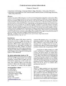
Figure 2. The Aplysia buccal feeding CPG in vitro. When driven by stimulation of the interneuron CBI-2 or of the esophageal nerve (EN), the CPG, residing in the paired buccal ganglia (photograph), generates feeding motor programs. The experimental records show two representative programs from the dataset in Figure 3, each with an intracellular recording from neuron B8 and extracellular recordings from two nerves, the I2 nerve and buccal nerve 2, whose activities are used as standard markers respectively of the protraction (red) and retraction (blue) phases of the program. It is then usual to classify the programs as ingestive or egestive depending on whether B8, a radula closer motor neuron, fires at higher frequency in the retraction phase (as in the top program) or the protraction phase (as in the bottom program), respectively. In this paper (as described in Text S1, Section 1.1), we have mapped the two B8 firing frequencies onto a single variable, the behavior B, that expresses the ingestive-egestive character of the programs along a single dimension, from B = 1 (most ingestive) to B = 21 (most egestive). On the right, all of the 466 programs in the dataset in Figure 3, then broken down into those elicited by CBI-2 or EN stimulation, are plotted along this dimension. Some programs exceed the limits of B = 1 or B = 21 because those limits are defined on average over all of the programs (see Text S1, Section 1.1). doi:10.1371/journal.pone.0003678.g002

Figure 2), whereas if the B8 neurons fire predominantly in protraction, the program is egestive (the bottom program in Figure 2).

These dynamics are revealed when the motor programs in Figure 2 are plotted over time in Figure 3. Proekt et al. performed three types of experiments, stimulating CBI-2 alone (Figure 3A), EN alone (B), or CBI-2 with an embedded period of EN stimulation (C), in the pattern represented by the ‘‘stimulus’’ variable S. In each case, the first programs were intermediate, with the behavior B close to zero. Then, as the stimulation continued, the programs progressively evolved in the ingestive direction, toward B = 1, with CBI-2 stimulation (filled circles), or in the egestive direction, toward B = 21, with EN stimulation (empty circles). When the stimulation was discontinued, the programs relaxed back toward B = 0. The evolution occurred over several minutes, over a number of programs and, in vivo, cycles of the feeding behavior, with what we will therefore call ‘‘slow’’ dynamics. When the programs were made strongly egestive by EN stimulation and the stimulation was then switched to CBI-2, the first CBI-2-elicited program remained strongly egestive, and subsequent programs evolved in the ingestive direction with the same slow dynamics (Figure 3C, segment ‘‘4’’). In other words, simply the starting point of the slow evolution of the CBI-2-elicited programs was displaced in the egestive direction (compare segments ‘‘2’’ and ‘‘4’’ of Figure 3C). Interestingly, however, the converse switch from CBI-2 to EN stimulation switched the programs from strongly ingestive to strongly egestive essentially immediately, with fast dynamics (Figure 3C, arrow ‘‘3’’), much faster than was their slow evolution with EN stimulation alone (compare arrows ‘‘1’’ and ‘‘3’’ in Figure 3, B and C). Evolution in the egestive direction was thus greatly accelerated by a previous ingestive history. We modeled these dynamics with a simple differential-equation model. The slow dynamics can be fully explained (blue curve in Figure 3) by a very simple ‘‘1D’’ model with just one dynamical variable, B itself, that relaxes slowly toward steady states at B = 1,

Dynamics of the feeding CPG It might be expected that the identity of the stimulus that triggers each motor program would at the same time specify the character of that program—that CBI-2 stimulation, the ingestive stimulus, would trigger ingestive programs, and EN stimulation, the egestive stimulus, would trigger egestive programs. Aplysia feeding would then be a purely stimulus-driven behavior. However, this is not the case. Figure 2, right, summarizes the ingestive-egestive character of 466 motor programs, elicited either by CBI-2 or by EN stimulation, recorded in vitro by Proekt et al. [39]—the dataset whose dynamics we will model and investigate in this paper. In anticipation of the modeling, we have already in Figure 2 mapped the B8 firing frequencies recorded by Proekt et al. onto a single normalized variable, the ‘‘behavior’’ B, that ranges from B = 1, indicating the most ingestive feeding motor program and, in vivo, the most ingestive feeding behavior, to B = 21, indicating the most egestive program and behavior (see supplementary Text S1, Section 1.1). Like the observed movements of the behavior in vivo, the motor programs span the entire ingestiveegestive range. Furthermore, both the CBI-2- and EN-elicited programs cover a large, and overlapping, part of the range. At different times, the same CBI-2 stimulation, in particular, can elicit a strongly ingestive or a strongly egestive program. Thus, as Proekt et al. [39,40] concluded, the character of the motor programs is not directly specified by the stimulus. Neither is it random, however, or independent of these stimuli. Rather, it is specified by the internal state of the feeding CPG at the moment of stimulation, which evolves in response to the stimuli with well-defined, history-dependent dynamics. PLoS ONE | www.plosone.org

3

November 2008 | Volume 3 | Issue 11 | e3678

Behavior from CNS Dynamics

Figure 3. The dynamics of the Aplysia feeding CPG. Data from the experiments of Proekt et al. [39], already mapped onto our model variables. In the buccal feeding CPG preparation in vitro, Proekt et al. stimulated either CBI-2 alone (A) EN alone (B), or CBI-2 with an embedded period of EN stimulation (C) in the pattern shown here, represented by the stimulus variable S. From each motor program elicited by the stimulation, Proekt et al. measured the B8 firing frequencies in protraction and retraction (see Figure S1 and Text S1, Section 6.1), here mapped onto the single ingestiveegestive dimension of the variable B. Each filled or empty circle (CBI-2 or EN stimulation, respectively) represents the mean6SE of 6–18 programs; altogether the dataset contains 466 programs. The red curve is the best fit (see Text S1, Section 1.4) of the 2D model (equations summarized above; for complete model specification see Text S1, Section 1.3). The blue curve shows the corresponding behavior of the 1D model, not an independent fit to the data but rather simply the behavior of the 2D model with the memory M set to 0 (see Text S1, Section 2). doi:10.1371/journal.pone.0003678.g003

21, and 0 in response to CBI-2, EN, and no stimulation, represented by S = 1, 21, and 0, respectively (blue equation in Figure 3; for details see Text S1, Section 2). B itself thus is the internal state of the feeding CPG as it is expressed in the ingestive-egestive character of the feeding motor programs and behavior. The 1D model fails at just one point: it cannot explain the one component of fast dynamics in the data. This requires a ‘‘2D’’ model with an additional dynamical PLoS ONE | www.plosone.org

variable, which we call the ‘‘memory,’’ M. To explain the data, M builds up with its own slow dynamics when B.0 and then, upon EN stimulation, accelerates the relaxation of B toward B = 21 (red equations in Figure 3; see Text S1, Sections 1.2 and 1.3). M thus ‘‘remembers’’ ingestive behavior and modifies accordingly subsequent egestive behavior. The red curves of B and M in Figure 3 show the best fit of the full 2D model to the data. 4

November 2008 | Volume 3 | Issue 11 | e3678

Behavior from CNS Dynamics

the true environment, too, is slow. The slow dynamics are thus adapted to a slow environment. The 2D model, however—the full model of the dynamics of the Aplysia feeding CPG—completely failed to perform this task (Figure 4C, right). With its fast dynamics in the egestive direction, the model tracked only egestive stimuli, not ingestive stimuli (Figure 4B, simulation 3). The model thus failed in a biologically significant manner: it failed to eat.

These dynamics of the feeding CPG are not confined to the CPG itself, but emerge in the contractions of the various muscles and the phasing of the movements of the buccal feeding apparatus [29]. The question now is, what kind of behavior, in what kind of environment, are these dynamics adapted for?

Task 1: prediction of an uncertain environment One plausible role of such dynamics might be to predict the true state of the environment, so that the appropriate behavior can be produced. The true state of the environment is often uncertain. The ‘‘true’’ environmental stimuli may be incomplete and ambiguous, and they are perceived by the nervous system through limited and noisy sensory channels (Figure 1). Furthermore, the nervous system must often prepare now to execute the behavior later, in a future environment that is, by definition, unknown. Thus the behavior cannot simply be driven by the immediately perceived stimulus. Instead, the dynamics of the nervous system can act as an internal model that predicts what the true state of the environment will most likely be when the behavior is executed, and furthermore—when the dynamics are those of a complete sensory-motor system such as the Aplysia feeding CPG—it does so already in behavioral terms, by automatically producing the appropriate behavior. Proekt et al. [39] proposed that the slow dynamics of the Aplysia CPG act in this manner, integrating the perceived stimulus over time to estimate the true environment and consequently predicting conservatively that, when the next motor program is triggered, the true environment will most likely not have changed from that estimate and neither should the behavior. Thus, in Figure 3C, after the EN stimulation has made the programs egestive, the next program remains egestive even when it is triggered by CBI-2 stimulation. How well do the dynamics of the Aplysia CPG in fact perform this role? We gave our CPG models such a predictive task in a simulated environment (Figure 4A). The environment consisted of a sequence of true stimuli, St, randomly switching between ingestive, egestive, and none, represented by St = 1, 21, and 0, respectively, with durations drawn randomly from a Gaussian distribution with mean t. To model the uncertain perception of the environment, the true stimulus St was then corrupted by fast random noise to give the perceived stimulus, Sp, so that at any moment there was a given probability that if St was 1, say, Sp was 0 or 21. The CPG model was stimulated only with the perceived stimulus Sp, yet its task was to match its behavior B as closely as possible to the true stimulus St. Performance was defined simply as the average difference between B and St (for further details see Text S1, Sections 3.1 and 3.2). Figure 4B shows three representative simulations and Figure 4C maps the performance of the two CPG models over a range of environments defined by the two parameters t, the characteristic time scale of the environment expressed in the durations of the true stimuli St, and f, the fraction of St perceived in Sp—the degree of certainty of the environment. Cool colors represent poor performance, warm colors good performance. Consider first the 1D model, incorporating only the slow dynamics. When the environment was faster—that is, when St switched on average faster—than the slow dynamics of the model, B did not follow St at all (Figure 4B, simulation 1), resulting in poor performance (left side of Figure 4C, left). But when the environment was slower than the model dynamics, B tracked St well, ignoring a significant degree of obscuring noise (Figure 4B, simulation 2), resulting in good performance (top right corner of Figure 4C, left). Thus, indeed, by not responding to the perceived stimulus immediately but rather integrating it over time, the slow dynamics can extract from it a good prediction of the true environment, provided that PLoS ONE | www.plosone.org

Task 2: biologically realistic ingestion and egestion of seaweed strips The failure of the 2D model in all environments defined by the two environmental parameters tested implied that, as far as these environments were concerned, Task 1 could not be the task to which the dynamics of the CPG are adapted. In developing a more relevant task, we were guided by a key feature of the dynamics themselves. While Task 1 was completely symmetric in the prevalence and order of ingestive and egestive stimuli, the observed CPG dynamics exhibit an asymmetric second-order coupling between ingestion and egestion. Egestion is facilitated by prior ingestion, but not vice versa. This presumably reflects the fact that, in vivo, egestion is evoked to expel inedible seaweed only if the seaweed has previously been ingested, but ingestion has no such prerequisite. We constructed a correspondingly asymmetric environment and task—indeed, by incorporating also the other basic facts of Aplysia feeding, a complete, biologically realistic feeding scenario. In this scenario (Figure 5A; for details see Text S1, Section 3.3), the true environment consists of a large population of seaweed strips, with lengths drawn from a Gaussian distribution with mean t, which the CPG model is to eat, necessarily sequentially, strip by strip. Intrinsically, all of the seaweed is edible, generating a true stimulus St = 1. However, because of the uncertain perception of the environment, as in Task 1, St reaches the model only intermittently, to a degree governed by the parameter f, as the perceived stimulus Sp. Stimulated by Sp, the model produces the behavior B, which now explicitly acts on the environment by translating to a rate of change of the position, P, on the current strip: ingestive behavior B.0 produces forward movement, and egestive behavior B,0 backward movement, along the strip. To eat, the model must move forward along the strip, and through the sequence of strips, as rapidly as possible since its performance is judged, in a biologically realistic manner, by the total length of seaweed eaten per time. In this scenario, therefore, the CPG model—now, indeed, essentially a simulated agent (cf. [6,14,41])— moves through the feeding environment, and consequently perceives that environment, in a manner that depends not only on the intrinsic properties of the environment, but also on its own actions in the environment. This task would be straightforward, were it not for the fact that, while most of the strips are ‘‘free,’’ some of them (25% in the simulations in this paper) are ‘‘attached’’ at the end so firmly that, when ingested, they cannot be broken off. The attachment point (symbolized by the black color of the ends of the attached strips in Figure 5 and other figures) generates an egestive true stimulus St = 21 and the corresponding Sp. The model must then—because this is tough seaweed that cannot be broken or cut anywhere along its length—egest the entire strip again, all the way back to the beginning, before it can continue to feed on another strip. The model cannot simply avoid ingesting the attached strips in the first place, because at the beginning, and through the ingestion of their entire length until they are found to be attached, or not attached, at the end, all strips appear identical, all intrinsically edible, with St = 1. This is a consequence of the fact that the 5

November 2008 | Volume 3 | Issue 11 | e3678

Behavior from CNS Dynamics

Figure 4. Simulations and performance of the 1D and 2D models in Task 1. A: Schema of the task, explained in Results. B: Steady-state excerpts from three representative simulations, with different values of the environmental parameters t, the time scale of the environment, and f, the fraction of the true stimulus St that is apparent in the noisy perceived stimulus Sp, and with either the 1D or the 2D model. In simulations 2 and 3, Sp is plotted sampled at 1/s, rather than 10/s as in simulation 1, to allow its structure to show through in these compressed plots. C: Performance of the 1D and 2D models, color-coded according to the scale shown on the right, over values of t ranging from 1 to 1000 s (note the log scale) and f ranging from 1/3, where Sp is pure random noise with no information at all about St, to 1, where there is no noise at all and Sp is identical to St (see Text S1, Section 3.2). The locations of the three simulations in B are marked. doi:10.1371/journal.pone.0003678.g004 PLoS ONE | www.plosone.org

6

November 2008 | Volume 3 | Issue 11 | e3678

Behavior from CNS Dynamics

Figure 5. Performance of the 2D and 1D models in Task 2. A: Schema of the task, explained in Results. B: Local ingestive stimulus and global egestive goal oppose each other, driving the behavior in opposite directions along the same seaweed strip. C: Performance of the 2D and 1D models, color-coded according to the scale shown on the right, over values of t ranging from 1 to 250 and f ranging from 0, where the true stimulus St is not perceived at all, to 1, where St is always fully perceived (see Text S1, Section 3.3). doi:10.1371/journal.pone.0003678.g005

The 2D model, with both slow and fast dynamics, was able to perform Task 2, over a sharply defined range of environments, exceptionally well, indeed with performance approaching the theoretical maximum (see Text S1, Section 3.3) of ,1/3 (Figure 5C, left). The 1D model, with only the slow dynamics, was not able to perform the task at all (Figure 5C, right).

model, like real Aplysia, perceives only the purely local St and Sp just from the current point of contact with the environment. This fact has another interesting consequence. In egesting an attached strip, the model soon loses contact with the point of attachment where St = 21 and begins to move back over portions of the strip that, when the model moved over them earlier in the forward direction, generated, and now generate again, the intrinsic ingestive stimulus St = 1. Nevertheless, the model must continue to egest, following an egestive ‘‘goal’’ that is contrary not just to the perhaps misperceived stimulus Sp, as in Task 1, but now even to the true stimulus St. We will refer to this as ‘‘goal-driven’’ behavior, as opposed to the simple ‘‘stimulus-driven’’ behavior when the goal agrees with St (Figure 5B). Thus, in Task 2, it is no longer sufficient to predict the true state of the local environment at any moment, because the behavior appropriate to the local environment at any moment may not be the best behavior overall. Instead of a series of local predictions, the system must make, rather, a global prediction of the properties of the entire seaweed strip. PLoS ONE | www.plosone.org

Performance emerges from an interaction of slow and fast dynamics The region of high performance in Figure 5C, left, is conspicuously curved. This is because the performance depends not on t or f separately, but on their product tf (see supplementary Figure S3 and the accompanying Text S1, Section 6.3). The performance is low when either t or f is small (in region ‘‘a’’), and increases as tf increases (from left to right, and bottom to top, through region ‘‘b’’). The highest performance occurs around tf