Predicting binaural speech intelligibility from signals estimated by a blind source separation algorithm Qingju Liu1 , Yan Tang2 , Philip J.B. Jackson1 , Wenwu Wang1 1
Centre for Vision, Speech and Signal Processing, University of Surrey, UK 2 Acoustic Research Centre, University of Salford, UK
[email protected],
[email protected], {p.jackson, w.wang}@surrey.ac.uk
Abstract State-of-the-art binaural objective intelligibility measures (OIMs) require individual source signals for making intelligibility predictions, limiting their usability in real-time online operations. This limitation may be addressed by a blind source separation (BSS) process, which is able to extract the underlying sources from a mixture. In this study, a speech source is presented with either a stationary noise masker or a fluctuating noise masker whose azimuth varies in a horizontal plane, at two speech-to-noise ratios (SNRs). Three binaural OIMs are used to predict speech intelligibility from the signals separated by a BSS algorithm. The model predictions are compared with listeners’ word identification rate in a perceptual listening experiment. The results suggest that with SNR compensation to the BSS-separated speech signal, the OIMs can maintain their predictive power for individual maskers compared to their performance measured from the direct signals. It also reveals that the errors in SNR between the estimated signals are not the only factors that decrease the predictive accuracy of the OIMs with the separated signals. Artefacts or distortions on the estimated signals caused by the BSS algorithm may also be concerns. Index Terms: blind source separation, speech intelligibility, objective intelligibility measures, noise
1. Introduction Objective intelligibility measures (OIMs, e.g. [1, 2]) are useful in providing reasonable and fast predictions of speech intelligibility in various adverse listening conditions. Therefore, they are widely used in place of resource-consuming listening experiments using human listeners in many fields such as acoustic design [3], hearing impairment [4] and algorithm optimisations for improving speech intelligibility [5]. With further extensions to binaural listening, OIMs are capable of dealing with more realistic listening situations [6, 7, 8]. However, the majority of state-of-the-art OIMs are doubleended. To make an intelligibility prediction, they require prior information about the original clean speech signal and the noise signal(s) or the speech+noise mixture, as well as the strict mixing process such as the signal-to-noise ratio (SNR). Their usability is therefore limited in many practical scenarios in which the original signals are not readily available, for example, when estimating intelligibility from speech signals recorded by a pair of microphones in noisy public places. While there are some established single-ended methods (e.g. [9]) for predicting speech quality directly from a processed/degraded signal, very few relevant studies seek to predict intelligibility without accessing individual speech and masker sources. In [10], a singleended method based on speech-to-reverberation modulation en-
ergy ratio (SRME) was proposed. With further improvements, it demonstrated high correlations with subjective data from a hearing-impaired cohort in noisy reverberant conditions [4]. However, the SRME metric may not be suitable for predicting intelligibility in fluctuating noise maskers, whose effects not only reduce the modulation depth of the speech signal, but also introduce stochastic disturbance to speech modulation. Predicting intelligibility directly from the speech+noise mixture may be difficult; an intermediate approach could be to estimate the source signals from the mixture – any doubleended OIM can then make a prediction using the estimated signals. For binaural recordings, the state-of-the-art blind source separation (BSS) methods [11, 12, 13] using interaural level difference (ILD) and interaural phase difference (IPD) have demonstrated good performance for two-channel source separation. These BSS methods can largely preserve binaural cues, as well as maintain the energy of each sound source, which is vital for speech intelligibility in noise. How well, then, can speech intelligibility be predicted single-endedly from the BSSseparated signals using existing OIMs, compared to the OIMs’ performance when using ground truth signals? The aim of this study is therefore to examine the performance of three binaural OIMs in predicting intelligibility from the outputs of a BSS algorithm, in both stationary and fluctuating noise maskers. The model predictions are compared with listeners’ sentence-level word identification rate in a perceptual listening experiment. As the BSS may not thoroughly preserve the original SNR, two different SNR compensation schemes are tested in order to improve the OIM performance with the BSSseparated signals.
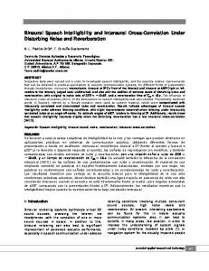
2. Proposed method Fig. 1 illustrates the framework of the proposed system. A BSS algorithm [11, 12, 13] is applied to extract both the target and masker signals. To implement real-time source separation and intelligibility prediction, the separation model is trained offline. The training data can be obtained at the stage of sound check Model parameter
Separation model
Binaural mixture
Binaural BSS
Intelligibility score target
Binaural OIM
masker
Figure 1: Flow chart of the proposed system. The thick arrows denote 2-channel data flow, while the solid lines represent model parameters. The yellow blocks operate online.
for example, so that the model will hold statistics of binaural features. Since the separation model is source positions- and the SNR level-dependent, these model parameters need to be estimated from the binaural mixture, from which the sources are estimated. As the output of the BSS stage, the separated signals are then fed into a binaural OIM for intelligibility estimation. 2.1. The binaural BSS algorithm As in [11], source signal from a certain direction arrives at two ears with different time delays and levels: L(t, f )/R(t, f ) = 10
α(t,f ) 20
√ −1β(t,f )
e
(1)
where L(t, f ) and R(t, f ) are the time-frequency (TF) representations of the left-ear and right-ear signals indexed by time frame t and frequency bin f . α(t, f ) and β(t, f ) denote interaural level difference (ILD) and interaural phase difference (IPD), respectively. Note that β is the frequency representation of the interaural time delay τ that β = [f τ ]π−π , which is mapped into the range of [−π, π]. If there is only one source signal coming from a specific direction θ, a Gaussian mixture model (GMM) can be employed to characterise the above bimodal features with the independence assumption between IPD and ILD: X IPD L(α, β|Ψθ ) = ϕτ |θ N (α|ΨILD (2) θ )N (β|Ψθ ) τ
where ϕτ |θ is the prior for P a signal coming from azimuth θ to yield the delay τ , and τ ϕτ |θ = 1. N (·|·) is the 2 Gaussian distribution, in which ΨIPD = {ξτ,f |θ ; στ,f θ |θ } contains the frequency-, azimuth- and delay-dependent mean ξτ,f |θ ILD 2 = {µf |θ ; ηf2 |θ } consists of and variance στ,f |θ , while Ψθ the frequency- and azimuth-dependent mean µf |θ and variance ILD ηf2 |θ . The parameter set, i.e. Ψθ = {ϕτ |θ , ΨIPD θ , Ψθ }, can be learned from binaural recordings containing only one signal from azimuth θ. Fig. 2 shows an example of parameter set Ψθ . For multiple sources coming from directions θi , i = 1, 2, · · · , I, based on the sparsity assumption that there is only one dominant signal at each TF point, we can adopt Eqn. 2 to X X L(α, β) = wi L(α, β|Ψθi ), s.t. wi = 1 (3) i
i
30
where wi is the weight of the i-th source coming from θi . The weight varies with the relative energy of each source in the mixture, e.g. the SNR level for one-target-one-masker cases. Given mixtures with known source directions θi , we can obtain the weight wi for each source at each TF point using an iterative expectation maximisation (EM) process. Note that, unlike the EM process applied to GMM models which estimates all the parameters, Ψθi is fixed to the parameter set directly extracted from the binaural mixture that contains only one source from direction θi . This avoids the overfitting problem when one signal is much weaker than the other signals, failing in yielding enough dominant features for convergence. When applying the trained BSS model {wi , Ψθi }Ii=1 to new binaural recordings, the TF separation mask Pfor the source coming from θi is generated as Mi (t, f ) = τ p(t, f, i, τ ), which is applied to both L(t, f ) and R(t, f ) to obtain the final binaural source estimate. 2.2. Binaural objective intelligibility metrics One recent and two standard OIMs with their binaural extensions were adopted as the backend intelligibility predictors. The binaural distortion-weighted glimpse proportion (BiDWGP). BiDWGP consists of two main components. The first one accounts for the local audibility of speech in noise by quantifying the number of speech regions with local SNR above a certain threshold, known as ‘glimpses’, on the spectrotemporal excitation pattern (STEP, [14]). The second component measures the effect of masker-induced distortions on speech envelope. To model binaural listening, glimpses and the frequency-dependent distortion factors are computed for both ears. The binaural interaction is accounted for by applying the gain computed as the binaural masking level difference (BMLD, [15, 16]) to the speech STEP when glimpses are defined. The better-ear effect is then simulated by combining glimpses from the two ears. The final intelligibility index is the sum of the numbers of glimpses in each frequency band, weighted by the distortion factor and band importance function. See [8] for more details. Note that, in this study it is assumed that the binaural signals of sources are directly accessible; the stage of estimating binaural signals from the single-channel signals engaged in [8] is omitted in the current implementation. Further comparisons on the outputs of the two implementations confirmed almost identical results.
ILD (dB)
20 10 0 -10 0
1
2
3
4
5
6
7
6
7
Frequency (kHz)
(a) ILD parameter ΨILD θ
IPD (rad)
π
-π 1
2
3
4
5
Frequency (kHz)
(b) IPD distribution p(·|θ) =
P
τ
ϕτ |θ N (·|ΨIPD θ )
Figure 2: The parameter set Ψθ for θ = π/3. (a) ILD: the solid line and the dotted lines are the mean µf |θ and deviations µf |θ ± ηf |θ , respectively. (b) IPD distribution calculated with ϕτ |θ and ΨIPD θ .
The binaural Speech Intelligibility Index (BiSII). BiSII extends its monaural standard measure – Speech Intelligibility Index [1] – to account for the better-ear effect and binaural interaction in binaural listening [6]. The apparent SNR in each frequency is computed for the two ears, taking the larger SNR between the two ears as the binaural SNR for that frequency. The frequency-specific BMLD gains are then added to the SNRs to obtain the effective SNRs, which are used for the final intelligibility index calculation. Otherwise, the implementation follows the standard procedure as described in [1]. The binaural Speech Transmission Index (BiSTI). An extension was introduced in [7] to enable the STI [2] to predict binaural intelligibility. Similarly to BiSII, for the better-ear effect the modulation transfer functions (MTFs) for each frequency band are calculated separately for both ears, and the larger value is then considered as the binaural MTF for that channel. The gain due to the binaural interaction is computed for frequencies of 0.5, 1 and 2 kHz using an method based on interaural crosscorrelation. More details are described in [7]. As implementa-
speech-shaped noise SNR
ISD
4
3
3
2
2
1
1
0
0
-1
-1 -10 20 -30 60 -90 90 120-150
BiSII
∆OIM
0.1
0.1
0
0
-0.1
-10 20 -30 60 -90 90 120-150 Masker azimuth (°)
-0.1
SNR
ISD
2
2
1
1
0
0
-1
-1 -10 20 -30 60 -90 90 120-150
BiSII
BiSTI
0.2
0.1
0.1
0
0
-0.1
SNR: -15 dB
-10 20 -30 60 -90 90 120-150
BiDWGP
0.2
-10 20 -30 60 -90 90 120-150 Masker azimuth (°)
4 3
BiSTI
0.2
SNR: -18 dB
3
-10 20 -30 60 -90 90 120-150
BiDWGP
0.2
competing speech 4
SNR: -6 dB
∆level (dB)
SNR: -9 dB
∆OIM
∆level (dB)
4
-10 20 -30 60 -90 90 120-150 Masker azimuth (°)
-0.1
-10 20 -30 60 -90 90 120-150 Masker azimuth (°)
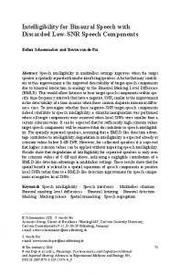
Figure 3: Comparisons of SNR and ISD levels (upper) and OIM predictions (lower) between the direct signal and that separated from SSN (left) and CS (right), calculated as the mean across the 220 sentences for each condition. tion in this study, the standard framework of the STI calculation [2] is used, except that the MTF is calculated using a phaselocked method [17], with a revised normalisation term [18].
3. Experiments The binaural samples used for testing were drawn from [8]. Harvard sentences were mixed with a stationary noise masker (SSN: speech-shaped noise) or a fluctuating noise masker (CS: female competing speech) at two SNR levels: -9 and -6 dB for SSN; -18 and -15 dB for CS. Both speech and masker sources were placed on a 2-metre radius. While the speech source was fixed ahead of the listener (θt = 0◦ ), the location of the masker varied in azimuth of θm ∈ [0, −10, 20, −30, 60, −90, 90, 120, −150, 180]◦ on a horizontal plane. The virtual anechoic sound field was simulated by convolving the single channel signals with corresponding binaural room impulse responses. In total, 32 conditions (2 maskers × 2 SNRs × 8 masker locations1 ) were tested. For each of the 32 conditions, a BSS model was trained offline. The required parameter set in Eqn. 2 was first calculated from the binaural mixtures for the target speech at θs and for the masker at each θm , respectively. Fig. 2 illustrates the learned parameter set for the competing speech masker at θm = π/3. After being processed by the BSS algorithm, the separated signals were then fed into the three binaural OIMs separately for calculating objective intelligibility scores. As the reference, objective scores were also computed from the signals of ground truth, which are referred to as the direct signals.
4. Evaluation Subjective listening tests [8] were first carried out in a word identification task for each of the simulated mixing conditions introduced earlier, which involved a group of 14 native British English speakers with normal hearing. The word-recognition score is used as the measure for the subjective binaural speech intelligibility. The 220 sentences used in the subjective listening tests in [8] were processed by the BSS for each of the 32 conditions. The upper row of Fig. 3 displays the difference be1 0◦ and 180◦ were excluded here as the target speech and the masker produce indistinguishable binaural features, resulting in poor BSS performance.
tween the direct signal and the separated signal in terms of SNR and interaural SNR difference (ISD), defined as ∆X = (Xdirect − Xseparated ), where X denotes the measurement used. The results suggest that while the spatial cues are well preserved (|∆ISD| < 0.5 dB), the BSS algorithm tends to underestimate the SNR level of the separated signals in all conditions. The average SNRs of the separated signals across masker locations and preset SNR levels are 1.7 dB lower in SSN and 2.7 dB lower in CS. Such underestimations are especially prominent when the masker is further off the central axis of the listener, i.e. 60◦ , ±90◦ and 120◦ , as well as 10◦ in CS. The lower row of Fig. 3 presents the ∆OIM for the three OIMs. Overall, the predictive patterns when using the separated signals reflect the impact due to the SNR underestimation. For individual OIMs, the Euclidean distance between the objective scores calculated from the the direct signals and the separated signals (row ‘Raw’ in Table 1) was computed for individual maskers (SSN and CS) separately and for the all 32 conditions (overall). Predictions of BiDWGP and BiSII, which quantify the masked-audibility directly using signal energy, are largely deviated from that of using direct signals. The BiSTI metric which measures modulation reduction, appears to be less sensitive to the SNR underestimation. Nevertheless, the effect due to the masker location is clear for all OIMs, especially in SSN. The objective predictions of the OIMs were further compared to the mean word identification rate (ranging between 20% and 93%, [8]) of 14 native British English speakers in the 32 conditions. The linear relationship between the objective and subjective intelligibility is measured as the Pearson correlation coefficient ρ and the error of pthe standard deviation of listener scores, defined as σe = σd 1 − ρ2 , where σd is the standard deviation of listener scores per condition. Table 2 exhibits the performance for all OIMs in sub-conditions, with the first shaded row showing the performance when the direct signals are used, as the ‘benchmark’. If the benchmark correlations are assumed to be the true performance of each OIM, any other higher or lower correlation relative to the benchmark should caused by the errors of the BSS algorithm when predicting intelligibility from the separated signals. With the separated signals (row ‘Raw’ in Table 2), BiSII can still maintain a linear relationship with listener performance reasonably well compared to its benchmarks, although it has produced smaller intelligibility indices than those with direct signals. However, while BiSTI only preserves its predictive
Table 1: Euclidean distance between the objective intelligibility scores computed from the direct and the separated signals. Raw
SNR Rec.
Sel. Comp.
SSN CS overall SSN CS overall SSN CS overall
BiDWGP
BiSII
BiSTI
0.28 0.64 0.70 0.16 0.34 0.37 0.15 0.55 0.57
0.73 0.49 0.88 0.61 0.27 0.67 0.68 0.43 0.80
0.10 0.15 0.17 0.10 0.03 0.10 0.04 0.10 0.11
Table 2: Objective-subjective correlation coefficients ρ (σe ) for using the direct signals (in grey) and the separated signals.
4.1. SNR rectification Having observed that the BSS algorithm leads to lower SNR for the separated signals, we also investigated the model performance when the SNR of the separated signals was rectified to match that of the direct signals. This process effectively reset ∆SN R to 0 dB for all conditions, resulting in the shortened Euclidean distance as shown in row ‘SNR Rec.’ of Table 1. The performance of each OIM is displayed in row ‘SNR Rec.’ of Table 2. BiSII and BiSTI achieved similar performance to their own benchmarks for individual maskers; there are some improvements in the performance of BiDWGP. However, perfectly restoring the SNR of the separated signals is almost impossible in practice without having prior knowledge of the true SNR. 4.2. Selective SNR compensation With the separated signals, the objective predictions seem more sensitive to the SNR underestimation when the masker is at 60◦ , ±90◦ and 120◦ than at other locations, as illustrated in Fig. 3. A solution would be to apply the gain only to these conditions. A set of 50 different sentences from the same corpus were used to explore the optimal gains. The optimisation was to maximise the Pearson correlation between the predictions of using the direct signals and using the separated signals. The higher the correlation, the closer the performance for the separated signals was to the true performance. The optimisation was conducted on the same two noise maskers but with an extended SNR range from -12 to 0 dB for SSN and -18 to -6 dB for CS, taking a 3dB step. The examined values for the gain were from 0.5 to 3 dB with a 0.5-dB step. The final optimal value of 1.5 dB was chosen as the point at which the mean correlation across the sub-conditions (SSN, CS and overall) was the best, based on the mean performance across all the three OIMs. However, it is worth noting that this procedure can only optimise the linear relationship between the predictions using the two approaches; it may not necessarily reduce the distance between the two types of predictions (see row ‘Sel. Comp.’ of Table 1). As demonstrated in row ‘Sel. Comp.’ of Table 2, by applying a constant 1.5-dB gain to the separated speech signals in the conditions where the masker is at 60◦ , ±90◦ and 120◦ , a remarkable improvement in the performance of BiDWGP was received, making it almost as accurate (ρ = 0.89) as when predicting from the direct signals (ρ ≥ 0.90). While BiSII lost some accuracy in CS (from 0.84 to 0.78), BiSTI maintained its benchmark performance for individual maskers. Nevertheless, all the OIMs still lack some robustness for cross-masker predic-
BiSII
BiSTI
benchmark
SSN CS overall
0.91 (0.09) 0.90 (0.05) 0.90 (0.07)
0.88 (0.10) 0.84 (0.07) 0.65 (0.13)
0.79 (0.13) 0.77 (0.08) 0.69 (0.12)
Raw
SSN CS overall SSN CS overall SSN CS overall
0.79 (0.13) 0.96 (0.04) 0.69 (0.12) 0.83 (0.12) 0.94 (0.04) 0.70 (0.12) 0.89 (0.10) 0.89 (0.06) 0.74 (0.11)
0.87 (0.10) 0.84 (0.07) 0.66 (0.13) 0.88 (0.10) 0.80 (0.07) 0.70 (0.12) 0.87 (0.10) 0.78 (0.08) 0.67 (0.13)
0.76 (0.14) 0.82 (0.07) 0.54 (0.14) 0.77 (0.13) 0.77 (0.08) 0.55 (0.14) 0.77 (0.13) 0.76 (0.08) 0.58 (0.14)
SNR Rec.
Sel. Comp. power in SSN, the accuracy of BiDWGP for separated signals decreases drastically in all sub-conditions.
BiDWGP
tions (i.e. overall) using separated signals. For DWGP, given its high benchmark overall correlation (ρ = 0.90), this is presumably due to the inconsistent distance shift from the objective scores computed from the direct signals in different maskers, as read from row ‘Sel. Comp.’ of Table 1.
5. Conclusions Three OIMs were employed to predict binaural speech intelligibility from the BSS-separated signals. Overall, except for across-masker prediction, the OIMs may provide similar predictive accuracy to their benchmark performance measured from the direct signals. As the outputs of the BSS algorithm, the SNR between the separated signals tends to be underestimated, especially when the masker is at 60◦ , ±90◦ and 120◦ in SSN as well as 10◦ in CS. The ideal SNR rectification does not recover the true performance for the OIMs, revealing that errors in SNR preservation are not the only issues for OIMs to make reliable intelligibility predictions from the separated signals; other aspects, such as the artefacts resulted from the BSS algorithm, may also play a role. The fact that selective SNR compensation largely benefited BiDWGP but not BiSII implies that, due to their different mechanisms, compensation to the estimated speech signal may need to be optimised individually for specific OIM for best performance. Further work will focus on identifying the kinds of distortions introduced by the BSS that OIMs can not account for, hence reduced predictive power of OIMs. Particularly, we should investigate the relationship between these distortions and different mechanisms of OIMs, and exploit this relationship in practical usages. For real-time processing there may be insufficient information on which BSS model is to train. Thus, a localisation model could also be employed at the early stage of the pipeline in order to estimate the source location. In addition, for an appropriate BSS model, statistics of the masker need also to be learnt online.
6. Acknowledgements This work was supported by the EPSRC Programme Grant S3A: Future Spatial Audio for an Immersive Listener Experience at Home (EP/L000539/1) and the BBC as part of the BBC Audio Research Partnership. Data underlying the findings are fully available without restriction, details are available from DOI 10.15126/surreydata.00811027.
7. References [1] ANSI S3.5-1997, “Methods for the calculation of the speech intelligibility index,” 1997. [2] IEC, “Part 16: Objective rating of speech intelligibility by speech transmission index (4th edition),” 2011, in IEC 60268 Sound System Equipment (International Electrotechnical Commission, Geneva, Switzerland). [3] G. Ballou, Handbook for sound engineers. 2013.
Taylor & Francis,
[4] J. F. Santos and T. H. Falk, “Updating the SRMR-CI metric for improved intelligibility prediction for cochlear implant users,” IEEE/ACM Trans. Audio, Speech, Language Process., vol. 22, no. 12, pp. 2197–2206, 2014. [5] C. Taal, R. C. Hendriks, and R. Heusdens, “Speech energy redistribution for intelligibility improvement in noise based on a perceptual distortion measure,” Computer Speech and Language, vol. 28, no. 4, pp. 858–872, 2014. [6] P. M. Zurek, Acoustical Factors Affecting Hearing Aid Performance. Allyn and Bacon, Needham Heights, MA, 1993, ch. Binaural advantages and directional effects in speech intelligibility, pp. 255–276. [7] S. J. van Wijngaarden and R. Drullman, “Binaural intelligibility prediction based on the speech transmission index,” J. Acoust. Soc. Am., vol. 123, no. 6, pp. 4514–4523, 2008. [8] Y. Tang, M. Cooke, B. M. Fazenda, and T. J. Cox, “A glimpsebased approach for predicting binaural intelligibility with single and multiple maskers in anechoic conditions,” in Proc. Interspeech, 2015, pp. 2568–2572. [9] L. Malfait, J. Berger, and M. Kastner, “P. 563&# 8212; The ITUT standard for single-ended speech quality assessment,” IEEE Trans. Audio, Speech, Language Process., vol. 14, no. 6, pp. 1924–1934, 2006. [10] T. H. Falk, C. Zheng, and W.-Y. Chan, “A non-intrusive quality and intelligibility measure of reverberant and dereverberated speech,” IEEE Trans. Audio, Speech, Language Process., vol. 18, no. 7, 2010. [11] M. I. Mandel, R. J. Weiss, and D. Ellis, “Model-based expectation-maximization source separation and localization,” IEEE Trans. Audio, Speech, Language Process., vol. 18, no. 2, pp. 382–394, February 2010. [12] A. Alinaghi, P. J. Jackson, Q. Liu, and W. Wang, “Joint mixing vector and binaural model based stereo source separation,” IEEE/ACM Trans. Audio, Speech, Language Process., vol. 22, no. 9, pp. 1434–1448, September 2014. [13] Q. Liu, W. Wang, P. J. B. Jackson, M. Barnard, J. Kittler, and J. Chambers, “Source separation of convolutive and noisy mixtures using audio-visual dictionary learning and probabilistic time-frequency masking,” IEEE Trans. Signal Process., vol. 61, no. 22, pp. 5520–5535, November 2013. [14] B. C. J. Moore, “Temporal integration and context effects in hearing,” J. Phonetics, vol. 31, pp. 563–574, 2003. [15] J. F. Culling, M. L. Hawley, and R. Y. Litovsky, “The role of headinduced interaural time and level differences in the speech reception threshold for multiple interfering sound sources,” J. Acoust. Soc. Am., vol. 116, no. 2, pp. 1057–1065, 2004. [16] J. F. Culling, M. L. Hawley, and R. Y. Litovsky, “Erratum: The role head-induced interaural time and level differences in the speech reception threshold for multiple interfering sound sources,” J. Acoust. Soc. Am., vol. 118, no. 4, p. 552, 2005. [17] R. Drullman, J. M. Festen, and R. Plomp, “Effect of reducing slow temporal modulations on speech reception,” J. Acoust. Soc. Am., vol. 95, no. 5, pp. 2670–2680, 1994. [18] R. L. Goldsworthy and J. E. Greenberg, “Analysis of speech-based speech transmission index methods with implications for nonlinear operations,” J. Acoust. Soc. Am., vol. 116, no. 6, pp. 3679– 3689, 2004.