Predicting Chaotic Time Series by Reinforcement Learning

Predicting Chaotic Time Series by Reinforcement Learning 1

T. Kuremoto1 , M. Obayashi1 , A. Yamamoto1 , and K. Kobayashi1 Dep. of Computer Science and Systems Engineering, Engineering Faculty,Yamaguchi Univ. Tokiwadai 2-16-1, Ube, Yamaguchi 755-8611, Japan {wu,obayashi,k}@csse.yamaguchi-u.ac.jp Abstract

Although a large number of researches have been carried out into the analysis of nonlinear phenomena, little is reported about using reinforcement learning, which is widely used in artificial intelligent, intelligent control, and other fields. Here, we consider the problem of chaotic time series using a self-organized fuzzy neural network and reinforcement learning, in particular, a learning algorithm called Stochastic Gradient Ascent(SGA). The proposed fuzzy neural network is similar to a radial basis function network(RBFN), but has self-organization ability dealing with its dynamical inputs,and provides stochastic outputs. The outputs are values of predicted time series, which called actions in reinforcement learning. After feeding some training data of chaotic time series to the initial frame of system, the structure and synaptic weights will be organized, and the predictor begins to provide correct dynamics of time series. Applying our proposed method to the Lorenz system, we obtained a high accuracy estimation of short-term prediction, and a reasonable result of long-term prediction.

1

Introduction

Studies on nonlinear phenomena in complex systems have been attracting many of researchers. Deterministic chaos, especially, comes to be the most important part of these studies recently, and either the basic theories or applications show us a large number of successful results [1, 2, 3, 4, 5]. In this paper, we would like to concern with the prediction of chaotic time series, and propose a new neural network model using reinforcement learning techniques. It’s too difficult to model complex, irregular signals of chaos by traditional methods of nonlinear analysis because of the large quantities of parameters, and its complexity of characteristics. So neural network models, as a kind of soft-computing methods, have been considered as effective nonlinear predic-

tors [2, 3, 4, 5]. Casdagli employed the radial basis function(RBF) network in chaotic time series prediction in early time [2]. Leung and Wang analyzed the structure of hidden-layer in RBFN, and proposed a technique called the cross-validated subspace method to estimate the optimum number of hidden units, and applied the method to prediction of noisy chaotic time series [4]. Oliveira ,Vannucci and Silva suggested a two-layered feedforward neural network, where the hyperbolic tangent activation function was chosen for all hidden units, the linear function for the final output unit, and obtained good results for the Lorenz system, Henon and Logistic maps [3]. Such of neural network models are not only developed on fundamental studies of chaos, but also applied in many nonlinear predictions, e.g., oceanic radar signals, financial time series, etc [4, 5]. Kodogiannis and Lolis compared the performance of some neural networks, i.e., Multi-layer perceptron(MLP), RBFN, Autoregressive recurrent neural network(ARNN), etc., and fuzzy systems, used for prediction of currency exchange rates, where RBFN gave a high degree of accuracy [5]. Meanwhile, reinforcement learning, a kind of goaldirected learning, is of great use for agent adapting unknown environments [6, 7]. When the environment belongs to Markov decision process(MDP), or Partially observable Markov decision process(POMDP), an agent acts some trial-and-error searches according to certain policies, and receives reward which can be considered as pleasure or pain of a living thing. Through the interactions between the environment and agent, both exploration and exploitation are carried out, agent approaches to goal more and more effectively. Though this kind of machine learning has been showing more and more contributions on artificial intelligence, optimal control theory and other fields, however, no speculation has taken place concerning the application in nonlinear prediction. This paper attempts to predict chaotic time series by an intelligent model which includes techniques of self-organization, fuzzy inference, and stochastic pol-

icy of reinforcement learning. In Section 2, we propose the architecture of prediction system and describe its detail process. Section 3 presents the application of proposed method on the Lorenz system, and results of prediction. Finally, in Section 4, the conclusion of this work will be reported.

2

Prediction System

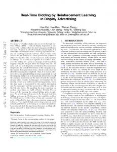
To extract the complex behavior characteristics of nonlinear signals, we employ a self-organized fuzzy neural network(Fig. 1). It is a RBF-like neural network because the membership functions are Gaussian distributions with different values of parameters. Because the number of hidden units in RBFN, which correspond to input patterns usually,is difficult to be determined [4], we consider fuzzy rules (similar to the model of Wang and Mendel [8]), and extend them to a self-organized system. Due to the output of neural network including stochastic parameters, stochastic gradient ascent(SGA) [7], is naturally served into the learning of our predictor. In fact, there are some hypothesize assert chaotic time series that we deal with are not some of determining chaos but artifact of stochastic process. We are not concerned here with this philosophical argument, just use a stochastic policy to determinate actions of prediction in the procedure of reinforcement learning.

2.1

2.2.1

Membership Function

To each element xi (t) of the input X(t), membership function Bij (xi (t)) is represented as ¾ ½ (xi (t) − mij )2 (3) Bij (xi (t)) = exp − 2 2σij where mij and σij are the parameters of mean and standard deviation of the Gaussian membership function in jth node, respectively. Initially, j = 1, and with increasing of input patterns, the membership functions will be added.

Reconstructed Inputs

According to the Takens embedding theorem, the inputs of prediction system on time t, can be constructed as a n dimensions vector space X(t), which includes n observed points with same intervals on time series y(t). X(t) = (x1 (t), x2 (t), · · · , xn (t)) (1) = (y(t), y(t − τ ), · · · , y(t − (n − 1)τ ) (2)

Figure 1: Architecture of prediction system

2.2.2

Fuzzy Inference

The fitness λk (X(t)) is an algebraic product of membership functions which connects to rule k.

where τ is time delay(interval of sampling), n is the embedding dimension. If we set up a suitable time delay and embedding dimension, then a track which shows the dynamics of time series will be observed in the reconstructed state space X(t) when time step t increases.

where o is the number of membership function, connects with k. o ∈ {1, 2, · · · , li }.

2.2

2.2.3

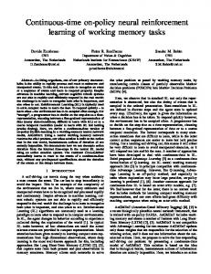
Self-organized Fuzzy Neural Network

Fig. 2 shows architecture of self-organized fuzzy neural network we proposed. The initial number of membership function and fuzzy rule is only 1, respectively.

λk (X(t)) =

n Y

Bio (xi )

(4)

i=1

Self-organization of Neural Network

For a step s on the time series, we calculate every membership function Bij (xi (s)), (i = 1, 2, · · · , n; j = 1, 2, · · · , li ) of inputs xi (s), and let sth node that has the largest value of Bij (xi (s)) connect to xi (s). In

PK σ(X(t), ωσk ) =

k=1

PK

λk ωσk

k=1

λk

(7)

tonaru. where µ is the mean of output,σ is its standard deviation. Weight ωµk andωσk are parameters concerning with inputs setX(t), and will be renew after learning. Thus, the output of neural network is according to a stochastic contribution, which is a prediction behavior. ½ ¾ 1 (ˆ y (t + 1) − µ)2 π(ˆ y (t + 1), W, X(t)) = √ exp − 2σ 2 2πσ (8) where yˆ(t + 1) is the value of one-step ahead prediction, produce by regular random numbers. W means weights ωµk andωσk . This function causes actions so it is called stochastic policy in reinforcement learning.

2.3 Figure 2: Self-organized fuzzy neural network this case,the input xi (s) shares existing membership function and fuzzy rule. Otherwise, if each node j of membership function has √ n Bij (xi (s)) < F (F¯ : T hreshold) (5) ,then a node supplement is necessary, a new membership will be added to correspond the input,li ← li + 1. To a new input set, if there is no any supplement of membership functions, existing membership functions connect with a same node of fuzzy rule, then supplement of rule is not necessary. Meanwhile, if there is a new membership function added, or if a disconnection between all existing nodes of membership functions with the node of fuzzy rule, then a node supplement is necessary, i.e., a new fuzzy rule will be added to correspond the node of membership function. So the connections between membership functions and fuzzy rules are multiple, and share/supplement operation is controlled by thresholds.

Reinforcement Learning of SGA

Reinforcement learning has recently been wellknown as a kind of intelligent machine learning [6, 7]. It needs not any model of operator but learns to approach to its gaol by observing sensing rewards from environments. Kimura and Kobayashi suggested an algorithm called stochastic gradient ascent(SGA), which respect to continuous action. Considering the characteristics of chaos, such as its orbital instability, boundedness, and self-similarity of attractor, it is appropriate to serve this stochastic approximation method to chaotic time series prediction system. SGA algorithm is given under. 1. Accept an observation X(t) from environment. 2. Predict a future data yˆ(t + 1) under a probability π(ˆ y (t + 1), W, X(t)). 3. Collate training samples of times series, take the error as reward ri . 4. Calculate the degree of adaption ei (t), and its history for all elements ωi of internal variable W . where γ is a discount(0 ≤ γ < 1). ei (t) =

2.2.4

Prediction Policy from Defuzzification

Integrate fuzzy rules with connection weight, fuzzy inference can be obtained. The output of signal can be considered as a new Gaussian distribution either, i.e., µ(X(t), ωµk ) =

Di (t) = ei (t) + γDi (t − 1)

(6)

(9) (10)

5. Calculate ∆ωi (t) by under equation. ∆ωi (t) = (ri − b)Di (t)

PK

k=1 λk ωµk PK k=1 λk

¡ ¢ ∂ ln π(ˆ y (t + 1), W, X(t)) ∂ωi

where b is a constant.

(11)

6. Improvement of policy:renew W by under equation. ∆W (t) = (∆ω1 (t), ∆ω2 (t), · · · , ∆ωi (t), · · ·) (12) W ← W + α(1 − γ)∆W (t)

(13)

where α is a learning constant,non-negative. 7. Advance time step t to t + 1,return to(1).

Figure 3: The Lorenz chaos

3

Application

We applied the proposed prediction system on time series of the Lorenz system to examine our method. Observe the Lorenz time series till 1500 steps, use the beginning 1000 steps to be training samples, then perform learning loops till prediction errors going to a convergence. After the architecture of system becomes stable, it is employed to predict data from 1001 step to 1500 step.

3.1

The Lorenz System

The Lorenz system, which is leaded from convection analysis, is composed with ordinary differential equations of 3 variableso(t), p(t), q(t). This paper uses their discrete difference equations (Equ. 14, 15, 16), and predicts the variable o(t)(Fig. 3). o(t + 1) = o(t) + ∆t · σ · (p(t) − o(t))

(14)

p(t + 1) = p(t) − ∆t(o(t) · q(t) − r · o(t) + p(t)) (15) q(t + 1) = q(t) + ∆t(o(t) · p(t) − b · q(t))

(16)

here,we set ∆t = 0.005, σ = 16.0, γ = 45.92, b = 4.0.

Figure 4: Numbers of membership functions and rules in self-organized fuzzy neural network with different input: (a)numbers of membership functions(fuzzy sets) (b)numbers of fuzzy rules

3.2

Parameters of Experiment

Parameters in every part of prediction system are reported here. 1. Reconstruction of input space by embedding(Equ.(1),(2)): Embedding dimension n : 3 Time delay τ : 1 (i.e.,in the case of input to be data of step 1,2,3, then the data of step 4 will be predicted.) 2. Self-organized fuzzy neural network: Initial value of weight ωµk :normal distribution ∈ (0, 1) Initial value of weight ωσk :0.5 Initial value of mij , σij in membership functions:0.0,15.0 Threshold of criterion for supplementary or share √ n of membership functions and rules F¯ : 0.99

Figure 5: Values of parameters in stochastic policy function with different learning times: (a)mean of µ (b)mean of σ 3. Reinforcement learning of SGA: Reward from prediction error rt is ½ 1 if |ˆ y (t + 1) − y(t + 1)| ≤ ε rt = −1 if |ˆ y (t + 1) − y(t + 1)| > ε . Limitation of errorsε:1.0 Discountγ:0.9 Learning constant: For weight ωµk , αωµk :0.003 For weight ωσk , αωσk :3.0E-6 For mean and standard deviation mij , σij,αmij , ασij :3.0E-6

3.3

Results of Experiment

Fig. 4 shows the numbers changing of nodes including membership functions(Fig. 4(a)) and fuzzy rules(Fig. 4(b)), respectively. As a consequence, the

Figure 6: Results of prediction with different learning times: (a)0 times (b)5000 times(c) 15000 times number of membership functions are 22, the fuzzy rules are 54. Fig. 5 shows the values changing of parameters in stochastic policy function π(ˆ y (t+1), W, X(t)) (Equ. 8). After about 11000 times learning,the learning of system goes to a convergence. and the value of average error(average of absolute value of each step’s prediction error) of 1000 steps comes to near 1.451(the range of time series values is about from -28.0 to 37). Fig. 6 demonstrates the change of prediction results with dif-

shows that the methods of soft-computing, such as neural networks and fuzzy techniques can be successfully used to predict the future state of nonlinear systems. The results of our experiment shows the proposed method is effective in deterministic chaotic time series prediction. The future work of this study will be comparisons of the performance with other prediction methods such as nonlinear modeling, RBFN, BP of MLP and so on, and we would like to go on to develop this system to treat noisy chaotic systems.

Acknowledgments This work was supported by MEXT KAKENHI (13450176 and 15700161). Figure 7: Prediction of non-learned data(short-term prediction: one-step ahead)

References [1] K. Aihara, T. Takabe and M. Toyoda, Chaotic neural networks, Physics Letters A, Vol.144, Issues 6-7, pp.333-340, 1990 [2] M. Casdagli,Nonlinear prediction of chaotic time series, Physica D: Nonlinear Phenomena Vol. 35, Issue 3, pp.335-356, 1989 [3] K. A. de Oliveira, A. Vannucci, E. C. da Silva, Using artificial neural networks to forecast chaotic time series, Physica A, No.284, pp.393-404, 1996

Figure 8: Prediction of non-learned data(long-term prediction: regressive prediction) ferent learning times. We used this system to predict the data from 1001 step to 1500 step of Lorenz time series those are not learned, obtained a good result with high accuracy(Fig. 7). Additionally, using the prediction values as the inputs of system, i.e., executing predictor regressively, we had a long-term prediction till 500 step, and results suggest the strong ability of our proposed system (Fig. 8).

4

Conclusion

We proposed an intelligent predictor in this paper, and demonstrated reinforcement learning is of great use to nonlinear phenomena analysis. This work also

[4] H. Leung, T. Lo, S. Wang, Prediction of Noisy Chaotic Time Series Using an Optimal Radial Basis Function, IEEE Trans. on Neural Networks, Vol. 12, No.5, pp.1163-1172, 2001 [5] V. Kodogiannis, A. Lolis, Forecasting Financial Time Series using Neural Network and Fuzzy System-based Techniques,Neural Computing & Applications, No.11, pp.90-102, 2002 [6] R.S.Sutton and A.G. Barto, Reinforcement Learning: An introduction,The MIT Press,1998 [7] H. Kimura, S. Kobayashi, Reinforcement Learning for Continuous Action using Stochastic Gradient Ascent , Intelligent Autonomous Systems, Vol.5, pp.288-295, 1998 [8] L. X. Wang, J. Mendel,Generating fuzzy rules by learning from samples, IEEE Trans. on System, Man and Cybernetics,Vol.22, Issue 6, pp.14141427, 1992