Predicting Climate Change using Response Theory: Global Averages ...

Predicting Climate Change using Response Theory: Global

arXiv:1512.06542v1 [physics.ao-ph] 21 Dec 2015

Averages and Spatial Patterns∗ Valerio Lucarini, Francesco Ragone, Frank Lunkeit December 22, 2015

Abstract The provision of accurate methods for predicting the climate response to anthropogenic and natural forcings is a key contemporary scientific challenge. Using a simplified and efficient open-source general circulation model of the atmosphere featuring O(105 ) degrees of freedom, we show how it is possible to approach such a problem using nonequilibrium statistical mechanics. Response theory allows one to practically compute the time-dependent measure supported on the pullback attractor of the climate system, whose dynamics is non-autonomous as a result of time-dependent forcings. We propose a simple yet efficient method for predicting - at any lead time and in an ensemble sense - the change in climate properties resulting from increase in the concentration of CO2 using test perturbation model runs. We assess strengths and limitations of the response theory in predicting the changes in the globally averaged values of surface temperature and of the yearly total precipitation, as well as their spatial patterns. We also show how it is possible to define accurately concepts like the the inertia of the climate system or to predict when climate change is detectable given a scenario of forcing. Our analysis can be extended for dealing with more complex portfolios of forcings and can be adapted to treat, in principle, any climate observable. Our conclusion is that climate change is indeed a problem that can be effectively seen through a statistical mechanical lens, and that there is great potential for optimizing the current coordinated modelling exercises run for the preparation of the subsequent reports of the Intergovernmental Panel for Climate Change. ∗

Paper prepared for the special issue of the Journal of Statistical Physics dedicated to the 80th birthday of Y.

Sinai and D. Ruelle.

1

1

Introduction

The climate is a forced and dissipative nonequilibrium chaotic system with a complex natural variability resulting from the interplay of instabilities and re-equilibrating mechanisms, negative and positive feedbacks and covering a very large range of spatial and temporal scales [1]. One of the outstanding scientific challenges of the last decades has been the attempt to provide a comprehensive theory of climate, able to explain the main features of its dynamics, describe its variability, and predict its response to a variety of forcings, both anthropogenic and natural [2]. The study of the phenomenology of the climate system is commonly approached by focusing on distinct aspects like: • wave-like features such Rossby or equatorial waves, which have enormous importance in terms of predictability and transport of, e.g., energy, momentum, and water vapour; • particle-like features such as hurricanes, extratropical cyclones, or oceanic vortices, which are of great relevance for the local properties of the climate system and its subdomains; • turbulent cascades, which determine, e.g. dissipation in the boundary layer and and development of large eddies through the mechanism of geostrophic turbulence. While each of these points of view is useful and necessary, none is able to provide a comprehensive understanding of the properties of the climate system. On a macroscopic level, one can say that at zero order the climate is driven by differences in the absorption of solar radiation across its domain. The prevalence of absorption at surface and at the lower levels of the atmosphere leads, through a rich portfolio of processes, to compensating vertical energy fluxes (most notably, convective motions in the atmosphere and exchanges of infrared radiation), while the prevalence of absorption of solar radiation in the low latitudes regions leads to the set up of the large scale circulation of the atmosphere (with the hydrological cycle playing a key role), which allows for reducing the temperature differences between tropics and polar regions with respect to what would be the case in absence of horizontal energy transfers [3, 4]. It is important to stress that such organized motions of the geophysical fluids, which act as negative feedbacks but cannot be treated as diffusive Onsager-like processes, typically result from the transformation of some sort of available potential into kinetic energy, which contrasts the damping due to a variety of dissipative processes. Altogether, the climate can be seen as a thermal engine able to transform heat into mechanical energy with a given efficiency, and

2

featuring many different irreversible processes that make it non-ideal [5, 6]. Besides the strictly scientific aspect, much of the interest on climate research has been driven in the past decades by the accumulated observational evidence of the human influence on the climate system. In order to summarize and coordinate the research activities carried on by the scientific community, the United Nations Environment Programme (UNEP) and the World Meteorological Organization (WMO) established in 1988 the International Panel on Climate Change program (IPCC). The IPCC reports, issued periodically about every 4-5 years, provide systematic reviews of the scientific literature on the topic of climate dynamics, with special focus on global warming and on the socio-economic impacts of anthropogenic climate change [7, 8, 2]. Along with this review effort, the IPCC defines standards for the modellistic exercises to be performed by research groups in order to provide projections of future climate change with numerical models of the climate system. A typical IPCC-like climate change experiment consists in simulating the system in a reference state (a stationary preindustrial state with fixed parameters, or a realistic simulation of the present-day climate), raising the CO2 concentration (as well as, in general, the concentration of other greenhouse gases such as Methane) in the atmosphere following a certain time modulation in a certain time window, and then fixing the CO2 concentration to a certain value to observe the relaxation of the system to a new stationary state. Each time-modulation of the CO2 forcing defines a scenario, and it is a representation of the expected CO2 increase resulting from a specific path of industrialization and change in land use. While much progress has been achieved, we are still far from having a conclusive framework of climate dynamics. One needs to consider that the study of climate faces, on top of all the difficulties that are intrinsic to any nonequilibrium system, the following additional aspects that make it especially hard to advance its understanding: • the presence of well-defined subdomains - the atmosphere, the ocean, etc. - featuring extremely different physical and chemical properties, dominating dynamical processes, and characteristic time-scales; • the complex processes coupling such subdomains; • the presence of a continuously varying set of forcings resulting from, e.g., the fluctuations in the incoming solar radiation and the processes - natural and anthropogenic - altering the atmospheric composition; • the lack of scale separation between different processes, which requires a profound revision

3

of the standard methods for model reduction/projection to the slow manifold, and calls for the unavoidable need of complex parametrization of subgrid scale processes in numerical models; • the impossibility to have detailed and homogeneous observations of the climatic fields with extremely high-resolution in time and in space, and the need to integrate direct and indirect measurements when trying to reconstruct the past climate state beyond the industrial era; • the fact that we can observe only one realization of the process. Since the climate is a nonequilibrium system, it is far from trivial to derive its response to forcings from the natural variability realized when no time-dependent forcings are applied. As already noted by Lorenz [9], it is hard to construct a one-to-one correspondence between forced and free fluctuations in a climatic context. Previous attempts on predicting climate response based broadly on applications of the fluctuation-dissipation theorem have had some degree of success [10, 11, 12, 13, 14], but, in the deterministic case, the presence of correction terms due to the singular nature of the invariant measure make such an approach potentially prone to errors [15, 16]. Adding noise in the equations in the form of stochastic forcing - as in the case of using stochastic parametrizations [17] in multiscale system - provides a way to regularize the problem, but it is not entirely clear how properties convergence in the zero noise. Additionally, one should provide a robust and meaningful construction of the model to be used for constructing the noise: a proposal in this direction is given in [18, 19, 1]. In this paper we want to show how climate change is indeed a well-posed problem at mathematical and physical level by presenting a theoretical analysis of how a general circulation model of intermediate complexity responds to simplified yet representative changes in the atmospheric composition mimicking increasing concentrations of greenhouse gases. We will frame the problem of studying the statistical properties of a non-autonomous, forced and dissipative complex system using the mathematical construction of the pullback attractor [20, 21], and will use as theoretical framework the Ruelle response theory [22, 15] to compute the effect of small time-dependent perturbations on the background state. We will stick to the linear approximation, which has proved its effectiveness in various examples of geophysical interest [16, 23]. The basic idea is to use a set of probe perturbations to derive the Green function of the system, and be then able to predict the response of the system to a large class of forcings having the same spatial structure. In this way, the uncertainties associated to the

4

application of the fluctuation-dissipation theorem are absent and the theoretical framework is more robust. Note that, as shown in [24], one can practically implement the response theory also to treat the nonlinear effects of the forcing. PLASIM [25], the climate model we use in this analysis, has O(105 ) degrees of freedom and provides a flexible tool for performing theoretical studies in climate dynamics. PLASIM is much faster (and indeed simpler) than the state of the art climate models used in the IPCC reports, but provides a reasonably realistic representation of atmospheric dynamics and of its interactions with the land surface and with the mixed layer of the ocean. The model includes a suite of efficient parametrization of small scale processes such as those relevant for describing radiative transfer, clouds formation, and turbulent transport across the boundary layer. In a previous work [23] we have considered a somewhat unrealistic set-up for the model, where the meridional oceanic heat transport was set to zero, with no feedback from the climate state. Such a limitation resulted in an extremely high increase of the globally averaged surface temperature resulting from higher CO2 concentrations. In this paper we extend the previous analysis by using a better model and by considering a wider range of climate observables able to provide a more complete picture of the climate response to CO2 concentration. The paper is organized as follows. In Section 2 we introduce the main concepts behind the theoretical framework of our analysis. We briefly describe the basic properties of the pullback attractor and explain its relevance in the context of climate dynamics. We then discuss the relevance of response theory for studying situations where the non-autonomous dynamics can be decomposed into a dominating autonomous component plus a small nonautonomous correction. In Section 3 we introduce the climate model used in this study, discuss the various numerical experiments and the climatic observables of our interest, and present the data processing methods used for predicting the climate response to forcings. In Section 4 we present the main results of our work. We focus on two observables of great relevance, namely the surface temperature and the yearly total precipitation, and investigate the skill of response theory in predicting the change in their statistical properties, exploring both changes in global quantities and spatial patterns of changes. We will also show how to flexibly use response theory for predicting when climate change becomes statistically significant in a variety of scenarios. In Section 5 we summarize and discuss the main findings of this work. In Section 6 we propose some ideas for potentially exciting future investigations.

5

2

Pullback Attractor and Climate Response

Since the climate system experiences forcings whose variations take place on many different time scales [26], defining rigorously what climate response actually is requires some care. It seems relevant to take first a step in the direction of considering the rather natural situation where we want to estimate the statistical properties of complex non-autonomous dynamical systems. Let us then consider a continuous-time dynamical system x˙ = F (x, t)

(1)

on a compact manifold Y ⊂ Rd , where x(t) = φ(t, t0 )x(t0 ), with x(t = t0 ) = xin ∈ Y initial condition and φ(t, t0 ) is defined for all t ≥ t0 with φ(s, s) = 1. The two-time evolution operator φ generates a two-parameter semi-group. In the autonomous case, the evolution operator generates a one-parameter semigroup, because of time translational invariance, so that φ(t, s) = φ(t − s) ∀t ≥ s. In the non-autonomous case, in other terms, there is an absolute clock. We want to consider forced and dissipative systems such that with probability one initial conditions in the infinite past are attracted at time t towards A(t), a time-dependent family of geometrical sets. In more formal terms, we say a family of objects ∪t∈R A(t) in the finitedimensional, complete metric phase space Y is a pullback attractor for the system x˙ = F (x, t) if the following conditions are obeyed: • ∀t, A(t) is a compact subset of Y which is covariant with the dynamics, i.e. φ(s, t)A(t) = A(s), s ≥ t. • ∀t limt0 →−∞ dY (φ(t, t0 )B, A(t)) = 0 for a.e. measurable set B ⊂ Y. where dY (P, Q) is the Hausdorff semi-distance between the P ⊂ Y and Q ⊂ Y. We have that dY (P, Q) = supx∈P dY (x, Q), with dY (x, Q) = inf y∈Q dY (x, y). We have that, in general, dY (P, Q) 6= dY (Q, P ) and dY (P, Q) = 0 ⇒ P ⊂ Q. See a detailed discussion of these concepts in, e.g., [20]. Note that a substantially similar construction, the snapshot attractor, has been proposed and fruitfully used to address a variety of time-dependent problems, including some of climatic relevance [27, 28, 29, 30]. In some cases, the geometrical set A(t) support useful measures µt (dx). These can be obtained as evolution at time t through the Ruelle-Perron-Frobenius operator [31] of the Lebesgue measure supported on B in the infinite past, as from the conditions above. Proposing a minor generalization of the chaotic hypothesis [32], we assume that when considering sufficiently

6

high-dimensional, chaotic and non-autonomous dissipative systems, at all practical levels - i.e. when one considers macroscopic observables - the corresponding measure µt (dx) constructed as above is of the SRB type. This amounts to the fact that we can construct at all times t a meaningful (time-dependent) physics for the system. Obviously, in the autonomous case, and under suitable conditions - e.g. in the case of of Axiom A system or taking the point of view of the chaotic hypothesis - A(t) = Ω is the attractor of the system (where the t− dependence is dropped), which supports the SRB invariant measure µ(dx). Note that when we analyze the statistical properties of a numerical model describing a non-autonomous forced and dissipative system, we often follow - sometimes inadvertently a protocol that mirrors precisely the definitions given above. We start many simulations in the distant past with initial conditions chosen according to an a-priori distribution. After a sufficiently long time, related to the slowest time scale of the system, at each instant the statistical properties of the ensemble of simulations do not depend anymore on the choice of the initial conditions. A prominent example of this procedure is given by how simulations of past and historical climate conditions are performed in the modeling exercises such as those demanded by the IPCC [7, 8, 2], where time-dependent climate forcings due to changes in greenhouse gases, volcanic eruptions, changes in the solar irradiance, and other astronomical effects are taken into account for defining the radiative forcing to the system. Note that future climate projections are always performed using as initial conditions the final states of simulations of historical climate conditions, with the result that the covariance properties of the A(t) set are maintained. Computing the expectation value of measurable observables for the time dependent measure µt (dx) resulting from the evolution of the dynamical system given in Eq. 1 is in general far from trivial and requires constructing a very large ensemble of initial conditions in the Lebesgue measurable set B mentioned before. Moreover, from the theory of pullback attractors we have no real way to predict the sensitivity of the system to small changes in the dynamics. The response theory introduced by Ruelle [22, 15] (see also extensions and a different point of view summarized in, e.g. [33]) allows for computing the change in the measure of an Axiom A system resulting from weak perturbations of intensity  applied to the dynamics in terms of the properties of the unperturbed system. The basic concept behind the Ruelle response theory is that the invariant measure of the system, despite being supported on a strange geometrical set, is differentiable with respect to . See [34] for a discussion on the radius of convergence (in terms of ) of the response theory.

7

In this case, instead, our focus is on saying that the Ruelle response theory allows for constructing the time-dependent measure of the pullback attractor µt (dx) by computing the time-dependent corrections of the measure with respect to a reference state. In particular, let us assume that we can write x˙ = F (x, t) = F (x) + X(x, t)

(2)

where |X(x, t)|  |F (x)| ∀t ∈ R and ∀x ∈ Y, so that we can treat F (x) as the background dynamics and X(x, t) as a perturbation. Under appropriate mild regularity conditions, it is possible to perform a Schauder decomposition [35] of the forcing, so that we express X(x, t) = P∞ k=1 Xk (x)Tk (t). Therefore, we restrict our analysis without loss of generality to the case where F (x, t) = F (x) + X(x)T (t). One can evaluate the expectation value of a measurable observable Ψ(x) on the time dependent measure µt (dx) of the system given in Eq. 1 as follows: Z



µt (dx)Ψ(x) = hΨi (t) = hΨi0 +

∞ X

(j)

j hΨi0 (t),

(3)

j=1

where hΨi0 =

R

µ ¯(dx)Ψ(x) is the expectation value of Ψ on the SRB invariant measure µ ¯(dx) (j)

of the dynamical system x˙ = F (x). Each term hΨi0 (t) can be expressed as time-convolution (j)

of the j th order Green function GΨ with the time modulation T (t): Z ∞ Z ∞ (j) (j) hΨi0 (t) = dτ1 . . . dτn GΨ (τ1 , . . . , τj )T (t − τ1 ) . . . T (t − τj ).

(4)

At each order, the Green function can be written as: Z τ τ (j) GΨ (τ1 , . . . , τj ) = µ ¯(dx)Θ(τj − τj−1 ) . . . Θ(τ1 )ΛS0τ1 . . . S0j−1 ΛS0j Ψ(x),

(5)

−∞

−∞

where Λ(•) = X · ∇(•) and S0t (•) = exp(tF · ∇)(•) is the unperturbed evolution operator while the Heaviside Θ terms enforce causality. In particular, the linear correction term can be written as: (1)

hΨi0 (t), =

Z

Z µ ¯(dx)

∞

dτ ΛS0τ Ψ(x)T (t − τ ) =

Z

0

∞

−∞

(1)

dτ GΨ (τ )T (t − τ ),

(6)

while, considering the Fourier transform of Eq. 6, we have: (1)

(1)

hΨi0 (ω) = χΨ (ω)T (ω), (1)

(7)

(1)

where we have introduced the susceptibility χΨ (ω) = F[GΨ ], defined as the Fourier transform (1)

of the Green function GΨ (t). Under suitable integrability conditions, the fact that the Green

8

function G(t) is causal is equivalent to saying that its susceptibility obeys the so-called KramersKronig relations [36, 16], which provide integral constraints linking its real and imaginary part, √ so that χ(1) (ω) = iP(1/ω) ? χ(1) (ω), where i = −1, ? indicates the convolution product, and P indicates that integration by parts is considered. See also extensions to the case of higher order susceptibilities in [37, 38, 24, 39]. As discussed in [16, 1, 23], the Ruelle response theory provides a powerful language for framing the problem of the response of the climate system to perturbations. Clearly, given a vector flow F (x, t), it is possible to define different background states, corresponding to different reference climate conditions, depending on how we break up F (x, t) into the two contributions F (x) and X(x, t) in the right hand side of Eq. 2. Nonetheless, as long as the expansion is well defined, the sum given in Eq. 3 does not depend on the reference state. Of course, a wise choice of the reference dynamics leads to faster convergence. Note that once we define a background vector flow F (x) and approximate its invariant measure µ ¯(dx) by performing an ensemble of simulations, by using Eqs. 3-6 we can construct the time dependent measure µt (dx) for many different choices of the perturbation field X(x, t), as long as we are within the radius of convergence of the response theory. Instead, in order to construct the time dependent measure following directly the definition of the pullback attractor, we need to construct a different ensemble of simulations for each choice of F (x, t). One needs to note that constructing directly the response operator using the Ruelle formula given in Eq. 6 is indeed challenging, because of the different difficulties associated to the contribution coming from the unstable and stable directions [40]; nonetheless, recent applications of adjoint approaches [41] seem quite promising [42]. Nonetheless, starting from Eqs. 6-7, it is possible provide a simple yet general method for predicting the response the system for any observable Ψ at any finite or infinite time horizon t for any time modulation T (t) of the vector field X(x),if the corresponding Green function or, equivalently, the susceptibility, (1)

is known. Moreover, given a specific choice of T (t) and measuring the hΨi0 (t) from a set of experiments, the same equations allow one to derive the Green function. Therefore, using the output of a specific set of experiments, we achieve predictive power for any temporal pattern of the forcing X(x). In other term, from the knowledge of the time dependent measure of one specific pullback attractor, we can derive the time dependent measures of a family pullback attractors. We will follow this approach in the analysis detailed below. While the methodology is almost trivial in the linear case, it is in principle feasible also when higher order corrections are considered, as long as the response theory is applicable [38, 24, 39].

9

We also wish to remark that in some cases divergence in the response of a chaotic system can be associated to the presence of slow decorrelation for the measurable observable in the background state, which, as discussed in e.g. [43], can be related to the presence of nearby critical transitions. Indeed, we have recently investigated such issue in [44], thus providing the statistical mechanical analysis of the classical problem of multistability of the Earth’s system previously studied using macroscopic thermodynamics in [45, 46, 47].

3

A Climate Model of Intermediate Complexity: the

Planet Simulator - PLASIM The Planet Simulator (PLASIM) is a climate model of intermediate complexity, freely available upon request to the group of Theoretical Meteorology at the University of Hamburg (https://www.mi.uni-hamburg.de/en/arbeitsgruppen/theoretische-meteorologie.html) and includes a graphical user interface facilitating its use. By intermediate complexity we mean that the model is gauged in such a way to be parsimonious in terms of computational cost and flexible in terms of possibility to explore widely differing climatic regimes [48]. Therefore, the most important climatic processes are indeed represented, and the model is complex enough to feature essential characteristics of high-dimensional, dissipative, and chaotic systems, as the existence of a limited horizon of predictability due to the presence of instabilities in the flow. Nonetheless, one has to sacrifice the possibility of using the most advanced parametrizations for subscale processes and cannot use high resolutions for the vertical and horizontal directions in the representation of the geophysical fluids. Therefore, we are talking of a modelling strategy that differs from the conventional approach aiming at achieving the highest possible resolution in the fluid fields and the highest precision in the parametrization of the highest possible variety of subgrid scale processes [2], but rather focuses on trying to reduce the gap between the modelling and the understanding of the dynamics of the geophysical flow [49]. The dynamical core of PLASIM is based on the Portable University Model of the Atmosphere PUMA [50]. The atmospheric dynamics is modelled using the primitive equations formulated for vorticity, divergence, temperature and the logarithm of surface pressure. Moisture is included by transport of water vapour (specific humidity). The governing equations are solved using the spectral transform method [51, 52]. In the vertical, non-equally spaced sigma (pressure divided by surface pressure) levels are used. The parametrization of unresolved

10

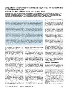
processes consists of long- [53] and short- [54] wave radiation, interactive clouds [55, 56, 57], moist [58, 59] and dry convection, large-scale precipitation, boundary layer fluxes of latent and sensible heat and vertical and horizontal diffusion [60, 61, 62, 63]. The land surface scheme uses five diffusive layers for the temperature and a bucket model for the soil hydrology. The oceanic part is a 50 m mixed-layer (swamp) ocean, which includes a thermodynamic sea ice model [64]. The horizontal transport of heat in the ocean can either be prescribed or parametrized by horizontal diffusion. In this case, we consider the second setting, as opposed to what explored in [23], because it is well known that having even a severely simplified representation of the large scale heat transport performed by the ocean improves substantially the realism of the resulting climate. We remind that the ocean contributes to about 30% of the total meridional heat transport in the present climate [4, 65, 66]. A detailed study of the impact of changing oceanic heat transports on the dynamics and thermodynamics of the atmosphere can be found in [67]. The model is run at T21 resolution (approximately 5.6o × 5.6o ) with 10 vertical levels. While this resolution is relatively low, it is expected to be sufficient for obtaining a reasonable description of the large scale properties of the atmospheric dynamics, which are most relevant for the global features we are interested in. We remark that previous analyses have shown that using a spatial resolution approximately equivalent to T21 allows for obtaining an accurate representation of the major large scale features of the climate system. PLASIM features O(105 ) degrees of freedom, while state-of-the-art Earth System Models boast easily over 108 degrees of freedom. While missing a dynamical ocean hinders the possibility of having a good representation of the climate variability on multidecadal or longer timescales, the climate simulated by PLASIM is definitely Earth-like, featuring qualitatively correct large scale features and turbulent atmospheric dynamics. Figure 1 provides an outlook of the climatology of the model run with constant CO2 concentration of 360 ppm and solar constant set to S = 1365 W m−2 . We show the long-term averages of the surface temperature TS (panel a) and of the yearly total precipitation Py (panel b) fields, plus their zonal averages [TS ] and [Py ]1 . Despite the simplifications of the model, one finds substantial agreement with the main features of the climatology obtained from observations and state-of-the-art model runs: the average temperature mono1

We indicate with [A] the zonally averaged surface value of the quantity [A].

11

tonically decreases as we move poleward, while precipitation peaks at the equator, as a result of the large scale convection corresponding to the intertropical convergence zone (ICTZ), and features two secondary maxima at the mid latitudes of the two hemispheres, corresponding to the areas of the so-called storm tracks [4]. As a result of the lack of a realistic oceanic heat transport and of too low resolution in the model, the position to the ICTZ is a bit unrealistic as it is shifted southwards compared to the real world, with the precipitation peaking just south of the equator instead of few degrees north of it. Beside standard output, PLASIM provides comprehensive diagnostics for the nonequilibrium thermodynamical properties of the climate system and in particular for local and global energy and entropy budgets. PUMA and PLASIM have already been used for several theoretical climate studies, including a variety of problems in climate response theory [23, 1], climate thermodynamics [68, 69], analysis of climatic tipping points [45, 44], and in the dynamics of exoplanets [46, 47].

3.1

Experimental Setting

We want to perform predictions on the climatic impact of different scenarios of increase in the CO2 concentration with respect to a baseline value of 360 ppm, focusing on observables Ψ of obvious climatic interest such as, e.g. the globally averaged surface temperature TS . We wish to emphasise that most state-of-the-art general circulation models feature an imperfect closure of the global energy budget of the order of 1 W m−2 for standard climate conditions, due to inaccuracies in the treatment of the dissipation of kinetic energy and the hydrological cycle [66, 1, 70, 71]. Instead, PLASIM has been modified in such a way that a more accurate representation of the energy budget is obtained, even in rather extreme climatic conditions [45, 46, 47]. Therefore, we are confident of the thermodynamic consistency of our model, which is crucial for evaluating correctly the climate response to radiative forcing resulting from changes in the opacity of the atmosphere. We proceed step-by-step as follows: • We take as dynamical system x˙ = F (x) the spatially discretized version of the partial differential equations describing the evolution of the climate variables in a baseline scenario with set boundary conditions and set values for, e.g., the CO2 = 360 ppm baseline concentration and the solar constant S = 1365 W m−2 . We assume, for simplicity, that system does not feature daily or seasonal variations in the radiative input at the top of

12

a)

b)

c) Figure 1: Long-term climatology of the PLASIM model. Control run performed with background value of CO2 concentration set to 360 ppm and solar constant defined as S = 1365 W m−2 : a) Surface temperature hTS i0 (in K); b) Yearly total precipitation hPy i0 (in mm); c) Zonally averaged values h[TS ]i0 (red line and red y−axis) and h[Py ]i0 (blue line and blue y−axis).

13

the atmosphere. We run the model for 2400 years in order to construct a long control run. Note that the model relaxes to its attractor with an approximate time scale of 20-30 years. • We study the impact of perturbations using a specific test case. We run a first set of N = 200 perturbed simulations, each lasting 200 years, and each initialized with the state of the model at year 200 + 10k, k = 1, . . . , 200. Let us choose as perturbation field X(x) the additional convergence of radiative fluxes due to changes in the atmospheric CO2 concentration. Therefore, such a perturbation field has non-zero components only for the variables directly affected by such forcings, i.e. the values of the temperatures at the resolved grid points of the atmosphere and at the surface. In each of these simulation we perturbed the vector flow by doubling instantaneously the CO2 concentration. This corresponds to having x˙ = F (x) → x˙ = F (x) + Θ(t)X(x). Note that the forcing is well known to scale proportionally with to the logarithm of the CO2 concentration [4]. • By plugging T (t) = Ta (t) = Θ(t) into Eqs. 6, we have that : d (1) (1) hΨi0 (t) = GΨ (t) dt

(8)

(1)

We estimate hΨi0 (t) by taking the average of response of the system over a possibly large number of ensemble members, and use the previous equation to derive our estimate of (1)

GΨ (t), by assuming linearity in the response of the system. In what follows, we present the results obtained using all the available N = 200 ensemble members, plus, in some selected cases, showing the impact of having a smaller number (N = 20) of ensemble members. It is important to emphasize that framing the problem of climate change using the formalism of response theory gives us ways for providing simple yet useful formulas for defining (1)

precisely the climate sensitivity ∆Ψ for a general observable Ψ, as ∆Ψ =