Which components of a large software system are the ... In a study on a large SAP Java system, .... development, the product is built and enhanced as well as.
Apr 1, 2009 - shopping mix e time increas omes the bottl ctions. The pr ..... [Kelly 2006] Terence Kelly, and Alex Zhang. Predicting perform- ance in distributed ...
Queen Mary, University of London. Mile End Road ... An important decision problem in many software projects is when ... Previously, this has required a custom-.
Bayesian Networks (BNs) in software engineering management. In our own ... to be taken into account, even when different evidence conflicts. Suppose that few ...
In a single replacement reaction, a single uncombined element replaces ... type:
combustion, oxidation, synthesis, decomposition, single replacement, double.
Some software products marketed by SAP AG and its distribu- tors contain
proprietary ..... the planning tool of SAP Trade Promotion Management, the
account ...
http://archive.eclipse.org/eclipse/downloads/. Figure 1 ..... file/package as defect-prone, otherwise as defect-free. ..... IEEE Transactions on Software Engineering,.
Apr 28, 2015 - Project management involves managing the project through- out the life ... In the information technology industry, project man- agement ..... New project. Table 3: Multiple regression results. Source. SS df. MS. Regression.
IBM Rochester, Minnesota, manufactures disk dri- ves on an assembly line. At various points in the man- ufacturing process, three phases of tests are performed.
Mar 15, 2018 - energy release rate at another crack nearby. Since this interaction is ..... amendment 11, EDF Energy, Gloucester, 2015. [3] 2013 ASME boiler ...
Jul 25, 2013 - 1Department of Physics, Applied Physics, and Astronomy, Rensselaer Polytechnic Institute, Troy, New York 12180, USA. 2Department of ...
Secondly, we assume that there are strictly positive lump-sum costs of ... lump sum costs of decision and price adjustment thus provides a simple and intuitively.
when licensing saP software. it presents practical examples outlining the different
.... and analysis, and saP Businessobjects Xcelsius® enterprise software for the
... employees who create reports and dashboards with the software, but also for ...
Center for Secure Information Systems ... confidentiality (as opposed to integrity) component of .... logical security level label provides information which.
is broadcast to all replica servers. The atomic broadcast primitive alleviates the need of a more ... abort rate. Finally, we compare the cost of a non-blocking.
tricks, data exclusivity for high levels of contaminants- would be barred ... 'Copgrighl" protections Corporate rules fo
... and download entire ebook libraries or basically hunt and peck in. driveUHEVD63280.fusionsbook.com/ search outcomes
Perfluorooctanoic acid and perfluorooctanesulfonate were predicted to be the ... biodegradation products of 17 and 27% of the perfluorinated sulphonic acid and ...
them (LefkoffHagius & Mason, 1993). Tom et al. (1998) found that consumers who indicated that they have previously purchased counterfeit goods hold attitudes ...
widespread and a part of daily life (Rutter &. Bryce, 2008; Baumgartel .... but more fashion clothing and accessories (Wah- ..... Women's Wear Daily. 192, 9.
Some authors suggested that organismic motivation theory like SDT potentially ... accessing media used by online retailers to sell fashion products; and without any experience in buying ..... Tonglet, M., Phillips, P. S. and Read, A. D. 2004.
experiment conducted at the University of Auckland (NZ) during the first semester of .... disadvantages, including students schedule issues [3],[5], pair incompatibility [3],[16] ..... [23] L. Thomas, M. Ratcliffe, and A. Robertson, Code warriors and
There was a problem previewing this document. Retrying... Download. Connect more apps... Try one of the apps below to op
only a fraction of the factors influencing the final product are taken into account. ...... [12] S. Kim, T. Zimmermann, E. J. Whitehead Jr., and A. Zeller. Predicting ...
predictions require a long failure history, which may not exist for the entity at hand; in fact, a long failure history is something one What is it that makes software fail? In an empirical study of the would like to avoid altogether. post-release defect history of five Microsoft software systems, we found that failure-prone software entities are statistically A second source of failure prediction is the program code itself: correlated with code complexity measures. However, there is no In particular, complexity metrics have been shown to correlate single set of complexity metrics that could act as a universally with defect density in a number of case studies. However, best defect predictor. Using principal component analysis on the indiscriminate use of metrics is unwise: How do we know the code metrics, we built regression models that accurately predict chosen metrics are appropriate for the project at hand? the likelihood of post-release defects for new entities. The In this work, we apply a combined approach to create accurate approach can easily be generalized to arbitrary projects; in failure predictors (Figure 1): WeZimmermann mine the archives of major particular, predictors obtained∗ from one project can also bePremraj Kim Herzig Rahul Thomas software systems in Microsoft and map their post-release failures significant for new, similar projects. Saarland University Saarland University University of Calgary back to individual entities. We then compute standard complexity [email protected][email protected][email protected] metrics for these entities. Using principal component analysis, we Categories and Subject Descriptors determine the combination of metrics which best predict the AndreasMaintenance, Zeller and Jürgen Heymann D.2,7 [Software Engineering]: Distribution, failure probability for new entities within the project at hand. Enhancement—version control.Saarland D.2.8 [Software Engineering]: University SAPweAGinvestigate Germany Finally, whether such metrics, collected from Metrics—Performance measures, Process metrics, Product [email protected][email protected] failures in the past, would also good predictors for entities of metrics. D.2.9 [Software Engineering]: Management—Software other projects, including projects be without a failure history. quality assurance (SQA)
ABSTRACT
Predicting Defects in SAP Products: A Replicated Study
ABSTRACT General Terms
1. Collect input data
Given a large body of Design, code, how do we know where to focus our Measurement, Reliability. quality assurance effort? By mining the software’s defect history, we can automatically Keywordslearn which code features correlated with defects in the past—and leverage these correlations new predicEmpirical study, bug database, complexityformetrics, principal tions: “Incomponent the past, high inheritance depth meant high number of deanalysis, regression model. fects. Since this new component also has a high inheritance depth, let us test1. it thoroughly”. Such history-based approaches work best INTRODUCTION if the newDuring component similar to software the components learned consumes from. softwareis production, quality assurance But how does learning effort. from history perform for projects high of a considerable To raise the effectiveness andwith efficiency variabilitythis between We itran studywhich on two SAP prod-We effort, components? it is wise to direct to athose need it most. therefore need to identify of those pieces of software which that are the ucts involving a wide spectrum functionality. We found mostpredicting likely to fail—and thereforeatrequire most of ourbut attention. learning and was accurate package level, not at product level. These suggest that topieces learncan from past past: de- If One source to results determine failure-prone be their fects, oneashould separate product component with software entitythe (such as ainto module, a file,clusters or some other component) was fail in thepredictions past, it is likely to do clusso in the similar functionality, andlikely maketoseparate for each Such to information be obtained from bug based databases— ter. Initialfuture. approaches form suchcan clusters automatically, on when coupled with version information, such that one similarityespecially of metrics, showed promising accuracy. can map failures to specific entities.
1.
Bug Database
As software quality assurance can account for more than half of the development time [3], it is important to focus this effort on those parts of the project which matter most—that is, those components with the highest number of defects, the highest risk of failure, or the highest potential damage. Allocating quality assurance efforts thus, is among the most important decisions of a quality assurance manager—a bad allocation can easily result in lack of quality, in wastage of resources, or both. To guide such decisions, predictions on the number of defects can be very helpful. Numerous studies have linked defects or defect density to code features—in particular, software complexity metrics [1, 19]. However, almost all studies predict pre-release defect density—that is, the number of defects before shipping the software to the customer. What managers need in addition, though, is a prediction of post-release defects—that is, the number of defects that ∗ Kim Herzig was an intern with SAP in the Fall of 2007 when this work was carried out.
Permission to make digital or hard copies of all or part of this work for personal or classroom use is granted without fee provided that copies are not made or distributed for profit or commercial advantage and that copies bear this notice and the full citation on the first page. To copy otherwise, to republish, to post on servers or to redistribute to lists, requires prior specific permission and/or a fee. Copyright 200X ACM X-XXXXX-XX-X/XX/XX ...$5.00.
Code Code Code
2. Map post-release failures to defects in entities Entity
Entity
Entity
3. Predict failure probability for new entities Entity
However, accurate
INTRODUCTION
Version Database
Predictor
Failure probability
Figure 1. After mapping historical failures to entities, we can use their metrics to predict failures new entities. Figure 1: complexity After mapping past defects to ofentities, we use their code metrics to predict defect counts for new entities _________________________________________________________________________________ (from [14]). *
Andreas Zeller was a visiting researcher with the Testing, Verification and Measurement Group, Microsoft Research in the actually escape into deployment, and therefore are most crucial to Fall of 2005 when this work was carried out.
guard against. Using code features to predict post-release defects is hard, since only a fraction of the factors influencing the final product are taken into account. What one can do, though, is to learn from history, e.g. which code features correlated with post-release defects in the past—and to assign most weight to those features that have the highest predictive power. This is the approach of Nagappan et al. [14] (referred to as MSR study, for Microsoft Research), showing high prediction accuracy for five Microsoft projects. The approach maps past defects to fixes, computes the past defect counts for entities, and then correlates defects with software complexity metrics to build a predictor for new entities (Figure 1). Unfortunately, learning from the past is appealing only if the past is representative of the future. In the MSR study, this meant that the model learned for Internet Explorer (IE) would be applicable for new IE components, but not for, say, new components for IIS, Microsoft’s Web Server; to make predictions for IIS components, one would have to learn from the IIS defect history. If a project spans a wide range of functionality (say, from Web browsing to Web serving), this raises the question how to successfully learn from history: Can we learn from the project as a whole, or do we need to decompose the project into smaller components—and, if so, what would be an appropriate level of granularity for this decomposition?
For these purposes, we have replicated the MSR study in an environment in which we expected to encounter a large variability within projects—precisely, two projects within SAP. The project domain, the development processes, the programming languages used are very different from the ones at Microsoft, and we were eager to see how learning from history would fare here. The contributions of this paper are as follows:
Table 1: Summary of the two SAP products investigated.
Developers # Statements # Added statements
1. We investigate whether the approach presented in the MSR study is applicable to alternate industrial settings—in particular, projects that integrate a wide range of functionality.
History available since History used
2. We explore prediction models at two granularity levels, namely packages and products.
Prediction method
3. We present prediction by package clusters, an improvement over the methods used in the original study that increases the usefulness of the approach. The remainder of this paper is organized as follows. After discussing related work (Section 2), we discuss the data collection (Section 3), followed by the experimental setup (Section 4). Section 5 presents the results obtained, followed by the threats to validity in Section 6 and a discussion in Section 7. Section 8 closes with conclusion and consequences.
2.
BACKGROUND
Predicting defects in software components has been addressed by a number of research studies in the past. Most of these studies used historical data, complexity metrics, or a combination of both to achieve their goals.
2.1
Historical Data
An emerging trend in defect prediction is to combine version repositories with bug databases [13, 15]. The concept of merging bug databases and version repositories has triggered a lot of work in the area, such as tracking source code entities responsible for defects in the past [5, 17, 20]. Schröter et al. [16] leveraged project’s history for defect prediction and demonstrated that using design data such as import relationships can reliably predict post-release defects. Also, Hassan et al. [8] and Kim et al. [12], both used dynamic caching algorithms, with the support of historical data, to predict 10% of the most defect prone source code entities with an accuracy of up to 95%. In contrast to them, most past work was carried out using static approaches.
2.2
Code Metrics
A larger proportion of research studies have used software metrics for defect prediction purposes. Previously, such metrics have shown to correlate with defects or defect density [1, 2, 4, 16, 19]. Basili et al. [1] were among the first to validate that object-oriented metrics are useful to predict defect density. Subramanyam and Krishnan [19] presented a survey on eight more empirical studies, all showing that object-oriented metrics significantly correlate with defects. Fenton et al. [4] showed that even code metrics developed for imperative, non-object-oriented code are capable to assess effort and quality of a software system. Ostrand et al. [15] used a set of 28 metrics and a negative binomial regression model to predict the most defect prone entities (top 20%) with an accuracy of up to 93%. Khoshgoftaar et al. [10, 11] used a quantitative software quality model to predict the defect rank order of software modules for most defect prone entities (top 20%) with an accuracy of up to 95%. But only very few research studies tried to predict post-release defects, i.e., defects occurring after software release. The MSR
Product A
Product B
> 500 ∼ 5.5 M ∼2M
> 500 ∼ 2.5 M ∼ 0.5 M
2002 2002–2006 (for all versions)
2002 2004–2005 (only for version N)
self prediction
forward prediction
study was amongst the first to predict post-release defects for industrial software projects. Using principal component analysis and linear regression, their results showed an overall rank correlation of up to 0.90 between predicted and observed defects. Besides their good correlation results, the MSR study also showed that no single prediction model is suitable to predict defects across several projects. Also, no metric(s) was observed to be universally applicable across different projects for defect prediction. Nevertheless, building prediction models based on source code metrics is promising, even if the resulting models have only local importance. In this paper, we follow the main steps (see Figure 1) used in the MSR study, making only minor adjustments to adapt the approach to the SAP development environment and the ABAP programming language.
3.
DATA COLLECTION
3.1
Researched Products
Our study is based on two major SAP products with sizes over two million lines of code and more than 500 developers each (see Table 1). To maintain confidentiality, we refer to these products as Product A and Product B. Originally, Product B contained approximately ten million lines of code, but to make its investigation manageable, we considered only those packages with high development activity in recent years (see # Added statements in Table 1). The included packages total to approximately 2.5 million lines of code. Both Product A and Product B are considerably larger than those products examined in the MSR study. At 306,000 lines of code, the largest Microsoft product is approximately eight times smaller than Product B and about eighteen times smaller than Product A. By choosing larger projects, we extend the scope of this replication to verify the scalability of the underlying MSR approach.
3.2
Characteristics of ABAP Code
The goal of this work was to predict post-release defect probabilities for ABAP products at SAP. The ABAP programming language not only allows programmers to use object-oriented elements like classes and interfaces, but also provides a variety of functional elements (e.g., function groups—a collection of functions and classes that share the same scope). Also, there is no separation between object-oriented and non-object-oriented coding in ABAP products. This mixture between object-oriented and non-object-oriented entities influenced many aspects of this study. Since both source code entity sets require different code metrics, we considered it necessary to study them separately. Thus, we classified source code entities as object-oriented or non-object-oriented, resulting in two separate, non-intersecting sets: CLASS and NON-CLASS, respectively. We dealt with function groups by separating object-oriented entities and adding them to CLASS. The remaining entities were
package level
class / function group level
metrics and defect data aggregated from below object-oriented metrics computed on this level
(defects predicted on this level)
include level
metrics aggregated from below defect data collected on this level
method level Non-object-oriented metrics computed on this level
Figure 2: Simplified representation of ABAP code entity levels. added to NON-CLASS. While traditional code metrics can be computed on both entity sets, object-oriented metrics can be computed for CLASS only. For NON-CLASS entities, these metrics were set to zero. Figure 2 shows the four most important granularity levels for ABAP. The bottom method level contains methods and functions on which non-object-oriented metrics were computed. The level above contains include entities containing multiple functions and methods. Classes and function groups are contained in the class / function group level. In contrast to Java, classes and function groups can be spread across multiple includes (and most of the times are). Metrics and defect data of lower levels are aggregated to this level. In addition, object-oriented metrics are computed on this level. The class / function group level is the lowest level containing all required data for defect prediction. Hence, we used it to conducted our defect prediction experiments. The top most package level can be compared to the package level for Java programs.
3.3
Defect Data
To base our prediction models on historical defect data, it was necessary to identify the source code entities that contained defects in the past. SAP’s defect database (CSS system) includes, for every fixed defect, a patch to fix it. Previously, Gurovic et al. [6] used these patches to count post-release defects for each entity at the include level, and later aggregated to the class/function group level. The latter is the level at which we conducted our experiments. To summarize, the defects taken into account by this study have the following properties: 1. The bug was filed in the CSS system. 2. The bug’s resolution is FIXED. 3. The entities affected by the fix can be queried from the CSS system.
3.4
Metrics Data
Not all metrics used in the MSR study could be applied to ours due to two reasons. First, not all metrics were applicable to ABAP
code because the projects in the MSR study were conducted using C++ and C#. Second, the current metrics computation framework at SAP, developed by Karg [9], posed several technical limitations. We extended this framework to compute a mixture of 28 traditional and object-oriented metrics on ABAP code (see Table 2 for a detailed list). Furthermore, we enriched our data set by adding suitable metrics like Halstead metrics [7] and database related metrics such as DB Read and DB Write. For each metric we present the name and computation level in the first and second columns of Table 2, respectively. The computation level indicates the level of granularity on which the metric was computed. The third column gives a short description for each metric. The fourth column states the aggregation function. Since nonobject-oriented code metrics are computed on method and function levels, these values must be aggregated to class and function group level to be combined with object-oriented metrics. The aggregation was performed using the aggregation functions: sum (Total), maximum (Max), and average (Avg). We have only reported the first two for brevity. The remaining three columns contain the aggregation functions and correlation values of the metrics with postrelease defects. The first of the three columns reports correlations for all entity types and the last two columns report correlation values for CLASS and NON-CLASS, respectively. Correlation values for those metrics not computable for NON-CLASS entities are set to zero. The discussion on Table 2 is deferred to Section 5.1.
4.
EXPERIMENTAL SETUP
In this section, we present a detailed overview of the experimental setup of this study. It is mainly adapted from the MSR study but contains some necessary modifications and extensions.
4.1
Prediction Models
We use linear regression to predict the number of defects for each entity. The 28 code metrics listed in Table 2 formed the inputs to the model; the predicted defect counts formed the output. Some metrics inter-correlated, which is a violation of one of the assumptions of regression models. For example, the number of basic blocks in a control flow graph is not independent of the number of arcs in the same control flow graph. To overcome this, we conducted a principal component analysis (PCA) on the data and used the top-50 of the 80 principal components for Product A and the top-60 for product B (Figure 3(a)). The difference in number of components is due to the fact that we wanted to have equally high percentages of cumulative variance for both products. A common argument against defect count prediction models is the lack of independence between defect count and code size. Nearly every metric correlates with number of statements. Hence, to show that our prediction models provide value, we compare the results to a size benchmark model that uses only number of statements as input to predict number of defects (Figure 3(b)).
4.2
Procedure
We chose two procedures to train and test our linear regression and size benchmark models: Self prediction. Training and testing sets are generated randomly using the same product version. Two-third of entities are used as training set while the remaining one-third entities comprise the testing set. Forward prediction. Training and testing sets are generated using successive product versions. Entities from version V are used as training set to predict those entities present in version V + 1.
Benchmark Prediction Model
Linear Regression Model
PCA
Metric Values
Linear Regression
Sort
Size
Predictor
(a) Linear Regression Model.
Benchmark Predictor
(b) Size Benchmark Model.
Figure 3: Prediction models used in the study. Of the two, the forward prediction setup is a closer simulation of reality. It delivers a better assessment of our approach, but requires data from two successive product versions. Unfortunately, for Product A data for only one version was accessible at SAP, which is why for Product A we could run only experiments based on the self prediction setup. For Product B, we had data from more than one version. Hence, we conducted experiments on it using the forward prediction setup.
4.3
Evaluation
Both the linear regression and size benchmark prediction models predict defect counts for arbitrary source code entities. But it is more realistic to rank source code entities by predicted defect counts to instead identify most defect prone entities. This way, we know which entities to test most. To evaluate the results, we sorted the entities by number of predicted and observed defect counts and computed the intersection between the top-20% entities. This amounts to the recall of the prediction models. Recall is the ratio of the entities in the intersection to the total number of top-20% entities observed as defect prone. A value of one is desirable and indicates that the prediction model identified all top-20% entities observed as defect-prone, while a value of zero indicates none of the top-20% entities were predicted. For those prediction models predicting post-release defects for the whole products (see Section 5.2), we sorted source code entities by observed and predicted number of defects. The order of entities defined a rank value for each entity. Using Spearman’s rank correlation coefficient [18], we then compared the observed and predicted ranks. The correlation describes how well observed and predicted ranks corresponded, the value lying between 1 and -1. A rank correlation coefficient equal to one would suggest that the rank sequences of observed and predicted number of defects completely coincide, while a coefficient equal -1 indicates that both rank sequences are completely opposite.
5.
RESULTS
The results are organized into four sections. We start with a discussion on correlations between the computed metrics and post-release defects. We then proceed to prediction models predicting defects at three levels of granularity—(a) product, (b) package, and (c) package clusters.
5.1
Metrics Correlation
Table 2 presents the correlations between CLASS and NON-CLASS entities and post-release defects. For most metrics, the correlation values for both types of entities were comparable, except for a select few for which they differed considerably, e.g., FanIn, FanOut, Weighted Methods. Another observation that can be made from Table 2 is that nonobject-oriented metrics have a higher distribution of correlation values than object-oriented metrics. While only two object-oriented
metrics have a correlation values greater than 0.50 (Weighted Methods, Response for class), six non-object-oriented metrics exceed a correlation value of 0.50 (Arcs, Blocks, Comments, Complexity, FanOut and Halstead). Although this indicates that non-objectoriented metrics are better predictors of post-release defects, we suspect that the higher correlation values are an artifact of more entities being available to compute non-object-oriented metrics. Also, it is likely that the metrics do not bear a linear relationship with post-release defects.
5.2
Prediction Models for Products
We began with building prediction models at the product level and created three different prediction models: (1) for all ABAP entity types, (2) for CLASS, and (3) for NON-CLASS only. Results from prediction at this level are presented in Table 3. It contains the R2 values for each of the three prediction models, as well as rank correlations between observed and predicted defect ranks for the top 5%, top 10%, and top 20% most defect prone entities, respectively. Additionally, the table lists the recall values for each prediction model. While the R2 values indicate poor prediction models, rank correlation and recall values show that the predictive accuracy of the prediction models are at par with comparable studies. Ostrand et al. [15] used negative binomial linear regression to predict the most defect prone entities (top 20%) on file level with a prediction recall of 71–93%. Hassan et al. [8] achieved a prediction recall of 45–82% and Kim et al. [12] of 73%–95% when using a caching approach and the top 10% as set of most defect prone entities. Khoshgoftaar et al. [10, 11] presented similar results when predicting the rank-order of modules using a quantitative software quality model. Comparing these results with recall values of 65–70% for Product A and 55–60% for Product B in this study, we are missing about 10% of prediction accuracy to get par. However, comparing the ranks between observed and predicted number of defects for all entities of each product (0.37–0.70) with those rank correlation coefficients presented by the MSR study (0.445–0.906), we see that our prediction models perform competitively, especially when considering that correlations above 0.70 were witnessed for only two of five Microsoft products. Comparing our linear regression models with the size benchmark model (Section 4.1), we gained an improvement of approximately 5%. Such an improvement may insignificant at first glance. In absolute terms, though, we can correctly predict approximately 500 additional defect locations. The recall values for Product A are comparable at top 5%, top 10%, and top 20% for both CLASS and NON-CLASS entities. However, this is not the case for Product B. The prediction models had higher recall values for CLASS entities than for NON-CLASS. This could be explained by the fact that we only included entities for Product B that showed recent development activity. Since most recent development activity is based on object-oriented code, more defects are found in them. On the other hand, NON-CLASS entities are older and more stable, manifesting lesser defects.
Table 2: Metrics correlations for ABAP source code with defect count. Complexity metrics for classes are not aggregated since the prediction models predict defect probabilities for this level of granularity. Correlation with post-release defects Metric Computation Level Description all entity types CLASS NON-CLASS Arcs
method
#arcs in control flow graph
Max Total
0.548 0.579
0.589 0.619
0.577 0.614
Blocks
method
#basic blocks in control flow graph
Max Total
0.503 0.540
0.507 0.549
0.517 0.600
Comments
method
#comments in function
Max Total
0.516 0.559
0.547 0.576
0.573 0.658
Complexity
method
McCabe’s cyclomatic complexity
Max Total
0.510 0.541
0.501 0.543
0.560 0.604
DB-Read
method
#statements reading from database tables
Max Total
0.275 0.283
0.246 0.250
0.210 0.220
DB-Write
method
#statements writing to database tables
Max Total
0.121 0.123
0.100 0.100
0.034 0.041
FanIn
method
#functions calling function
Max Total
0.287 0.287
0.093 0.093
0.444 0.463
FanOut
method
#functions called by function
Max Total
0.148 0.158
0.527 0.560
0.160 0.160
Halstead’s Difficulty
method
based on #operators and #operands, see [7]
Max Total
0.518 0.550
0.578 0.607
0.560 0.569
Parameters
method
#parameters in function
Max Total
0.246 0.332
0.263 0.460
0.305 0.431
Afferent Coupling
class
#classes in foreign packages used by class
0.091
0.158
n/a
Class In-Coupling
class
#classes using class
0.084
0.180
n/a
Class Out-Coupling
class
#classes used by class
0.086
0.344
n/a
Class Usage Indicator
class
#static methods / #methods
0.096
0.206
n/a
Efferent Coupling
class
#classes in foreign packages using class
0.157
0.300
n/a
Impl. Interfaces
class
#implemented interfaces by class
-0.032
0.012
n/a
Inheritance Depth
class
#superclasses of class
-0.038
-0.006
n/a
Interface Methods
class
#interface methods implemented by class
-0.018
0.059
n/a
Maintainability Index
class
derived from Halstead metrics
0.096
0.146
0.237
Overwritten Methods
class
#direct overwritten methods by class
0.038
-0.008
n/a
Response for Class
class
#methods or functions called by class
0.494
0.575
0.570
Subclasses
class
#child classes of class
0.033
0.065
n/a
Weighted Methods
class
sum of method complexities in class
0.555
0.622
0.600
Table 3: Product Prediction Results: Regression, Rank Correlation and Recall Product A Product B
The last section showed that the predictions for post-release defects for the products had moderate predictive power. To explain these results, we examined the data more closely at the product and the package level. At the package level, we observed that for packages belonging to a product, the metrics correlated differently to one another with post-release defects. Thus, prediction models at the product level have conflicting data that distorts the training of the model. Also, we again examined the projects considered in the MSR study and noted that these projects have focus on one single domain (InternetExplorer → web browsing, NetMeeting → network communication, DirectX → computer graphics). In contrast, each SAP product offers a much wider range of services leading to many packages with markedly different domains grouped together to perform as a single product. Hence, we chose to instead build prediction models for each package to investigate if accuracy improves considering that the package contents are more uniform. But this is possible only if the packages have a certain minimum size and a sufficient number of post-release defect reports to allow building reliable prediction models. For this, we selected the ten largest packages of Product A that (a) had over 10,000 statements, (b) contained over 100 function groups and classes, and (c) had the highest defect densities. For Product B, we similarly selected the packages except for using including packages with more than 60 function groups and classes instead of 100. This was necessary because we investigated only a small part of Product B. The recall values for these package prediction models are presented as percentages and visualized using bars, as illustrated in Figure 4. Black values represent recall values of the linear regression model. Gray bars present the results from the size benchmark model (Table 3(b)). Longer bars indicate higher recall values, i.e., higher prediction accuracy. The corresponding percentages are reported on the right side of the bars. Table 4 presents the recall values for each package when predicting the top 20% most defect prone entities. For each product, we present results from the top 10 packages with the largest number of statements (listed in column three of Table 4). The packages are made anonymous as a–j, prefixed by the containing product and a separating dot (.) in the first column. The packages in the table are
graphical comparison of recall values
exact prediction recall values
Figure 4: Recall value representation sorted by decreasing order of defect density, but due to confidentiality reasons, we do not report their values in the table. This allows us to evaluate if there exists any relationship between the performance of the prediction models and the packages’ defect densities. The prediction accuracy itself is reported in the last column of the figure, as illustrated in Figure 4. We defer the explanation of the cluster column to Section 5.4. Sixteen of the twenty packages performed better than the size benchmark model, having an average prediction improvement of approximately 20%. Comparing results from prediction models on products and constituent packages, we gained 24% of accuracy for Product A and 26% of Product B using packages. In cases where prediction models showed no improvement over the benchmark, they performed at least as well, except in the case of A.f. The average recall of the prediction models is approximately 71% for all packages investigated (i.e., including packages not listed in the table). The average recall for Product A was 62%, marginally below the overall product recall. But the recall for some of Product A’s packages increased up to 75% and even higher for Product B. For the latter, some prediction models predicted up to 92% of the top 20% most defective entities.
5.4
Prediction Models for Package Clusters
In the last section, we observed that building prediction models at the package level, rather than product level, increases prediction accuracy. However, a result of this is numerous prediction models for each product. For example, Product A comprises 450 packages and we built a prediction model for each. Although this can be reliably automated, it comes at immense computational expense and is more difficult to manage and analyse. To reduce the number of prediction models per product, we built package clusters based on correlations between the metrics and
Table 4: Prediction Results at Package Level (Fix alignment) Package Cluster NOS Prediction Reliabilities for top 20%
Table 5: Prediction Results using Package Clusters Cluster # packages NOS Recalls Clusters for Product A
post-release defects. As mentioned above, at least in part, the overall product prediction models did not work because of different metric correlations between packages. We leveraged this information to group packages into clusters using the following steps: (1) Compute metric correlations at the package level. (2) Sort the packages by correlations and pick the top seven packages with the highest correlation. (3) Add these packages into set P. (4) Starting with the first package in P, we group all packages having a top metrics intersection size of three or more into one cluster C. If no such package exists, C contains only the first package P. (5) Remove those packages from P that were added to C in step 4. (6) Repeat steps 4 and 5 until P is empty. The computation of package clusters can be automated. Varying thresholds for the number of metrics in the top list (in our case seven) and the required intersection size (in our case three) may
result in different package clusters. But in any case, one package can only belong to one cluster at a time. Within a cluster C, the following holds: ∀A, ∀B ∈ C : |set(A) ∩ set(B)| ≥ 3 where A and B are packages and set(X) is the set of names of the seven most significant correlation metrics in package X. We report the results from the prediction models on package clusters in Table 5. The first column in the table reports the clusters represented using symbols. In total, using the above rules, we generated ten different clusters using the packages listed in Table 4—the cluster column in the table states the cluster in which the package belongs. Back in Table 5, the second column presents the number of packages present in the cluster. The third column presents the sum of the number of statements (NOS) in the constituent packages, while the last column presents the results. Here again, we present prediction accuracy using the visualisation illustrated in Figure 4—except that in this table, the black bar represents the prediction accuracy of the model on clusters, while the gray bar indicates the average prediction accuracy of all constituent packages from Table 4. For example, cluster α contains packages A.c, A.d, A.e, A.f, A.g, A.i. The reported value for the cluster in Table 5 is the average accuracy for all six packages computed from Table 4. Contrary to our expectation that prediction models on the package clusters will be inferior, we observed in fact they performed as well as the average prediction accuracy for packages, for a few cases even better (except for cluster θ). Thus, using clusters, we reduced the number of prediction models by 40–60%, or in other words: we cut the number of required prediction models to half without loosing prediction accuracy. Further improvement may be possible if we choose appropriate comparison thresholds in steps (2) and (4) mentioned above.
6.
THREATS TO VALIDITY
As any empirical study, this study has limitations that must be considered when interpreting its results.
Threats to external validity. These threats concern our ability to generalize from this work to
other industrial practice. In this study, two SAP products have been examined. It is possible that the examined products or parts of it may not be a representative for other products of SAP and other companies. It may also be the case that the presented prediction models only work for products similar to the two products under investigation. Different domains, product standards, and software processes all may influence defects—and come up with different results. Due to these threats, we consider our experiments as a proof of concept, but advise users to run an evaluation as described in this work before putting the technique to use.
Threats to internal validity. These threats concern our ability to draw conclusions about the connections between independent and dependent variables. We identified four specific threats:
7.
In the beginning, we replicated the MSR approach as such, but the results were not convincing. We improved on the predictive performance by switching to package prediction models which resulted fairly good prediction reliability of up to 92% of the most defective entities. This step forced us to compute a large number of prediction models per product. To compensate this shortcoming, we introduced prediction models based on package clusters. Each cluster contains packages with similar metric correlations, only. Not only did this reduce the number of prediction models by 40-60%, but also obtained the average predictive power observed for package prediction models in nearly every case. One may wonder why product prediction models did not show the expected predictive power in contrast to package prediction models. We identify two possible reasons: • First, it turned out that different packages of the investigated SAP products have different sets of code metrics that correlate with post-release defects. This may be explained by the fact that large software products contain multiple application layers serving different application duties. In contrast, the products investigated by the MSR study were considerably smaller in number of statements and were strongly focused on a single domain (e.g. Browsing ↔ Internet Explorer, Rendering ↔ DirectX).
• The defect data is incomplete. Collecting the post-release defect data, we used an approach developed by the Quality Governance & Production Group of SAP. We made no tests to verify the correctness of this data. We do know that there are post-release corrections to source code that are not covered by this approach. However, we believe that the error rate does not influence the predictive power of the described model. This assumption may be wrong and it may be the case that using another information pool, the prediction results may vary from those presented in this paper. • The metrics framework may have limitations. As mentioned before, this paper is based on a metrics computation framework by Karg [9]. There are some unresolved issues concerning this framework that—from our point of view—do not have a great influence to the above presented results. The biggest issue recognized so far is the fact that the framework ignores all macro entities. Since the fraction of entities representing macros is very small, we expect to ignore this fraction not to have any impact. Nevertheless, it may be the case that our expectation is wrong or that there might be undetected issues concerning this framework. • Source code Entities change their names. Source code entities are identified by their TADIR entry name. TADIR is the name of the database table containing information about all source code entities. The TADIR name of each entity is unique and can be used as identification key. When changing this name or other TADIR attributes of the entity, the history of this entity cannot be mapped to the entity anymore. In this case, the validation of the predicted post-release defects fails even if the real value has been predicted. • The implementation may have errors. A final source of threats is that our implementation could contain errors that affect the outcome. To control for these threats, we ensured that the prediction tools had no access to the data to be predicted or any derivative thereof. We also did careful cross-checks of the data and the results to eliminate errors in the best possible way.
Threats to construct validity. These threats concern the appropriateness of our measures for capturing our dependent variables, i.e., the number of defects of a component. This was justified at length when discussing the statistical approach.
DISCUSSION AND LESSONS LEARNED
• A second argument may be based on the product level itself. At SAP, the depth of granulates is deep and the distance between product level and actual source might be too long to preserve the measured source code properties. The four levels shown in Figure 2 are exceeded by at least four levels to the top and by more intermediate levels in between. All in all, we thus confirm our initial assumption that learning from the past is appealing only if the past is representative of the future. The more specific the domain we can learn from, the better the predictor. While learning from entire products may be too general for SAP, learning from individual packages provides good predictors that are applicable to existing components as well as to future components within that package.
8.
CONCLUSION AND CONSEQUENCES
When calibrated with defect history, software complexity metrics can accurately predict the number of post-release defects. For projects with a wide range of functionality, as explored in our study, it is advisable to separate the project into subsystems such as packages, and to learn and predict defects for each subsystem separately. Obviously, the finer the granularity, the more specific the prediction will be, and the higher the predictive power. By using a fully automated approach, as in the present paper, one can evaluate with different levels of granularity and choose the best balance between generality and accuracy. Using software metrics to predict defects is straight-forward, as they are easy to acquire, and easy to apply. However, when it comes to defect prediction, metrics are merely symptoms of hidden factors that make software more or less reliable. Just as one can detect and cure diseases by symptoms alone, we can make appropriate predictions. It is our duty, though, to further investigate these hidden factors— how to characterize them, how to measure them, and how to leverage them for recommendations as early as possible. Two important starting points we would like to investigate is architectural metrics (in particular when considering large-scale products like SAP) as
well as the age of source code entities, which has been shown to have an enormous effect on reliability prediction [12, 15]. We look forward to incorporate such factors and to make automated predictors even more attractive. In the long term, we shall need much more data from the software development process. We will thus concentrate on collecting such data from modern programming environments [21] and further relating it to effort and quality. We do not believe that such automated recommendations will ever surpass human expertise— even if we could collect all process data ever available. However, recommendations can certainly complement expertise—and can provide the necessary findings to avoid bad decisions.
9.
REFERENCES
[1] V. R. Basili, L. C. Briand, and W. L. Melo. A validation of object-oriented design metrics as quality indicators. IEEE Trans. Softw. Eng., 22(10):751–761, 1996. [2] A. B. Binkley and S. R. Schach. Validation of the coupling dependency metric as a predictor of run-time failures and maintenance measures. In ICSE ’98: Proceedings of the 20th international conference on Software engineering, pages 452–455, Washington, DC, USA, 1998. IEEE Computer Society. [3] B. W. Boehm. Software Engineering Economics. Prentice Hall PTR, Upper Saddle River, NJ, USA, 1981. [4] N. E. Fenton and S. L. Pfleeger. Software Metrics: A Rigorous and Practical Approach. PWS Publishing Co., Boston, MA, USA, 1998. [5] M. Fischer, M. Pinzger, and H. Gall. Populating a release history database from version control and bug tracking systems. In ICSM ’03: Proceedings of the International Conference on Software Maintenance, page 23, Washington, DC, USA, 2003. IEEE Computer Society. [6] D. Gurovic and U. Gebhardt. Treasure in Silver Lake. SAP AG Germany (Walldorf), publicly not available. [7] M. H. Halstead. Elements of Software Science (Operating and programming systems series). Elsevier Science Inc., New York, NY, USA, 1977. [8] A. E. Hassan and R. C. Holt. The top ten list: Dynamic fault prediction. In ICSM ’05: Proceedings of the 21st IEEE International Conference on Software Maintenance (ICSM’05), pages 263–272, Los Alamitos, CA, USA, 2005. IEEE Computer Society. [9] L. Karg. Evaluierung des Six-Sigma-Ansatzes und relevanter Kennzahlen am Beispiel der SAP AG unter Betrachtung der Problembereiche Messung von ABAP-Softwareartefakten und Vorhersage von Fehlern. Master’s thesis, Technische Universität Darmstadt, 2006. In cooperation with SAP AG Germany (Walldorf), publicly not available. [10] T. Khoshgoftaar and E. Allen. Predicting the order of fault-prone modules in legacy software. In ISSRE ’98: Proceedings of the The Ninth International Symposium on Software Reliability Engineering, page 344, Washington, DC, USA, 1998. IEEE Computer Society. [11] T. M. Khoshgoftaar and E. B. Allen. Ordering fault-prone software modules. Software Quality Control, 11(1):19–37, 2003. [12] S. Kim, T. Zimmermann, E. J. Whitehead Jr., and A. Zeller. Predicting faults from cached history. In Proceedings of the 29th International Conference on Software Engineering, pages 489–498, May 2007.
[13] N. Nagappan and T. Ball. Use of relative code churn measures to predict system defect density. In ICSE ’05: Proceedings of the 27th international conference on Software engineering, pages 284–292, New York, NY, USA, 2005. ACM. [14] N. Nagappan, T. Ball, and A. Zeller. Mining metrics to predict component failures. In ICSE ’06: Proceeding of the 28th international conference on Software engineering, pages 452–461, New York, NY, USA, 2006. ACM. [15] T. J. Ostrand, E. J. Weyuker, and R. M. Bell. Predicting the location and number of faults in large software systems. IEEE Transactions on Software Engineering, 31(4):340–355, 2005. [16] A. Schröter, T. Zimmermann, and A. Zeller. Predicting component failures at design time. In Proceedings of the 5th International Symposium on Empirical Software Engineering, pages 18–27, September 2006. ´ [17] J. Sliwerski, T. Zimmermann, and A. Zeller. When do changes induce fixes? In MSR ’05: Proceedings of the 2005 international workshop on Mining software repositories, pages 1–5, New York, NY, USA, 2005. ACM. [18] C. Spearman. Demonstration of formulae for true measurement of correlation. The American Journal of Psychology, 18(2):161–169, 1907. [19] R. Subramanyam and M. S. Krishnan. Empirical analysis of ck metrics for object-oriented design complexity: Implications for software defects. IEEE Trans. Softw. Eng., 29(4):297–310, 2003. ˇ [20] D. Cubrani´ c and G. C. Murphy. Hipikat: recommending pertinent software development artifacts. In ICSE ’03: Proceedings of the 25th International Conference on Software Engineering, pages 408–418, Washington, DC, USA, 2003. IEEE Computer Society. [21] A. Zeller. The future of programming environments: Integration, synergy, and assistance. In FOSE ’07: 2007 Future of Software Engineering, pages 316–325, Washington, DC, USA, 2007. IEEE Computer Society.