Keywords-Cloud Service, IaaS Profit Maximization, Behavior. Prediction models, Combinatorial Optimization. I. INTRODUCTION. Cloud computing is ...
Predicting Dynamic Requests Behavior in Long-term IaaS Service Composition Sajib Mistry, Athman Bouguettaya, Hai Dong, and A. K. Qin School of Computer Science & Information Technology RMIT University, Melbourne, Australia Email:{sajib.mistry, athman.bouguettaya, hai.dong, kai.qin}@rmit.edu.au Abstract—We propose a novel composition framework for an Infrastructure-as-a-Service (IaaS) provider that selects the optimal set of long-term service requests to maximize its profit. Existing solutions consider an IaaS provider’s economic benefits at the time of service composition and ignore the dynamic nature of the consumer requests in a long-term period. The proposed framework deploys a new multivariate HMM and ARIMA model to predict different patterns of resource utilization and Quality of Service fluctuation tolerance levels of existing service consumers. The dynamic nature of new consumer requests with no history is modelled using a new community based heuristic approach. The predicted long-term service requests are optimized using Integer Linear Programming to find a proper configuration that maximizes the profit of an IaaS provider. Experimental results prove the feasibility of the proposed approach. Keywords-Cloud Service, IaaS Profit Maximization, Behavior Prediction models, Combinatorial Optimization.
I. I NTRODUCTION Cloud computing is increasingly becoming the technology of choice as the next-generation platform for conducting business. Big companies such as Amazon, Microsoft, Google and IBM are already offering Infrastructure-as-aService (IaaS), Platform-as-a-Service (PaaS) or Software-asa-Service (SaaS) solutions in the cloud market [1]. Typically, an IaaS provider delivers Virtual Machine (VM) services to SaaS applications by providing services based on a fixed amount of resources (CPU, Memory, Network Bandwidth, etc.). For example, the IaaS provider Rackspace can host around 80,000 machines and the specifications of each machine is similar to a Dell PowerEdge 2970 [2]. The IaaS provider usually advertises certain Quality of Services (QoSs) (e.g., availability, response time, etc.) in the Service Level Agreement (SLA). SLA violations may incur penalties for the provider [1]. For example, Rackspace refunds 30% of a consumer bill if the availability of its services is less than 99% in a month [3]. As the number of IaaS cloud consumers (SaaS providers) are increasing, it is difficult to satisfy all consumer requests when considering resource constraints and SLA violations. The provider-consumer relationship between IaaS and SaaS providers is long-term and economically driven [4].In the cloud, a large proportion of services are provisioned long-term that are billed monthly or yearly instead of hourly. IaaS providers encourage long-term service requests by advertising cheaper prices on reserved resources. For example, a consumer can save up to 53% in a 3 year reservation plan compared to the on-demand scheme in Amazon EC2 [2]. Naturally, an IaaS provider receives long-
term service requests from different types of consumers. The provider should analyze the long-term profitability by composing service provisioning based on these requests before accepting them. We define the long-term service composition from the provider’s perspective as selecting an optimal set of long-term service requests that will maximize the provider’s objective functions (e.g., revenue and profit) while considering resource constraints and SLA violation penalties. To the best of our knowledge, existing approaches only consider the composition of shortterm service requests to achieve a trade-off between profit maximization and consumer satisfaction [5], [6], [7]. These approaches optimize the allocation of available resources at the time of compositions and maximize the profit in that time point. These approaches are not applicable to the long-term composition as the functional and non-functional requirements in the long-term service requests may change over time [4]. Due to the dynamic nature of the SaaS applications (e.g., multi-tenancy, changes in business requirements, etc.), a fixed set of requirements are not often applicable over a period of time. Figure 1(b) and (c) depicts the possible long-term (1 year) QoS and resource requirements from three different types of SaaS applications. As short-term compositions select consumer requests based on only current requirements, the selected requests may not be profitable in the future. We identify the following long-term factors that are missing in short-term compositions and incorporate them in the proposed framework: 1. Dynamic behavior of consumer requests in a longterm period: SaaS providers’ run-time service requests may be different from the initial requests. Such dynamism may occur in resource utilization, QoS fluctuation tolerance level and early contract termination. Generally, SaaS providers estimate the required long-term IaaS resources and add headroom over these estimates. This may lead to gross underutilization of IaaS resources in the runtime [8]. The underutilized resources can actually be allocated for other suitable consumer requests to maximize the profit. If other requests are unavailable, the operation cost can be reduced by turning off the under-utilized resources to save power. Consumers may early terminate contracts for various reasons [9]. In this situation, the allocated resources of the exiting consumers can be used for new consumer requests to maximize the profit. Similarly, QoS fluctuation tolerance is another important runtime behavior of consumer requests. When the IaaS provider advertises QoS, some consumers may tolerate some extent of QoS fluctuations in delivered services [9]. The IaaS
provider therefore prefer consumers who are more likely to tolerate QoS fluctuations to reduce possible SLA violation penalties. 2. Long-term economic model of IaaS provider: According to [2], electricity cost is the most influential variable in an IaaS provider’s operation cost. Electricity price, employee wages, etc. fluctuate in a long-term basis and is influenced by demand and supply phenomena. The future operation cost of a service cannot be easily measured using current environment variables. Hence, an economic model is required for estimating the long-term profit generated by a service composition. 3. Optimal resource allocation in different arrival models of requests: When an IaaS provider has certain resource constraints, it is important to allocate resources optimally to maximize the profit. For example, composing only CPUintensive services may early run out the CPU quota and under-utilize the networking resources. Besides, composing services using over-provisioned resources may cause SLA violations. The future service demand also needs to be considered in the time of composition. In the deterministic situation, all the long-term requests are available at the time of composition. The type of requests and their arrival time can be accurately predicted by the composer using deterministic models. In the stochastic situation, both the request type and their arrival time are stochastic in nature. Therefore, a service composition task is to determine whether to offer a service to a request or reserve it for a forthcoming more profitable request. In this paper, a new IaaS service composition framework is proposed by considering the deterministic arrival of service requests. The stochastic arrival situation will be studied in the future. The key task of this framework is to predict the dynamic behavior of the consumer requests for the optimal composition. According to [8], the long-term consumer behavior on resource utilization can be represented as highfrequent, seasonal-trending or regime changing time series. SaaS providers such as Video Stream Services are likely to follow seasonal-trending or regime changing patterns [8]. Resource utilization time series of stock market SaaS applications generally follow high frequent patterns [10]. It is difficult to use a specific model to realize different patterns. Besides, service requirement attributes (VMs and QoSs) are often correlated and multivariate in nature [4]. Hence, we propose a new multivariate Hidden Markov Model (HMM) and Auto Regressive Integrated Moving Average (ARIMA) model to predict the high frequent or seasonal-trending long-term behavior of service requests based on historical evidences. In the case of new consumer requests without historical data, a novel community based bootstrapping method is devised to predict the future service usage. Once the incoming requests is transformed by projecting the dynamic behavior, we model the profit maximization problem using Integer Linear Programming (ILP) [11] by considering resource constraints (CPU, memory and network
bandwidth) and penalty caused by SLA violations. Due to the page limit, we are not addressing the provider’s longterm economic model in this paper. Instead a profit model is developed by using a short-term economic model in [2] and assuming that it remains constant in a long-term period. The key contribution of our research is a new service composition framework for IaaS providers. The novelty of the framework is summarized as: 1) The use of multivariate analysis on a HMM and ARIMA model for predicting the future QoS fluctuation tolerance level, resource utilization and early exit patterns of the existing consumers, and a community based bootstrapping method to predict the dynamic behavior of new consumer requests. 2) An ILP based solution for profit maximization taking transformed requests as inputs and considering resource constraints as well as SLA violation penalties. The paper is structured as follows: the related work, service composition framework and prediction model are discussed in Section II, III and IV respectively. The optimization process, experiments and conclusion are presented in Section V, VI and VII respectively. II. R ELATED W ORK Existing approaches for service composition from provider’s perspective mainly focus on the short-term single service provision rather than multiple service provisions. Resource allocation algorithms for SaaS providers are proposed in [5] to minimize the infrastructure cost and SLA violations. The algorithms are designed to ensure that SaaS providers are able to manage the dynamic demands of customers. A distributed architecture for the resource management is proposed in [6], [7] to prevent under-utilization and overutilization of resources by Multiple Criteria Decision Analysis. We propose a service composition framework that considers long-term service requests. A HMM and queuing models are considered in resource planning to predict QoS performance in [12]. Statistical analysis is performed to estimate the resource utilization in [13]. K-means clustering approach is applied for intelligent resource provision management in [14]. ARIMA [15] is the most commonly used model in auto regressive time-series analysis. An ARIMA based cloud workload prediction is proposed in [16]. An Artificial Neural Network (ANN) is designed to predict workload for massively multiplayer online game in the cloud [17]. As QoS and resource attributes have inherent correlations, existing approaches lack multivariate analysis for better predictions of the requests’ behavior. The predicted requests are composed into an optimization process. Linear Programming (LP), ILP, Quadratic Programming (QP) are mostly used optimization techniques [11]. An ILP model for short-term resource allocation and task scheduling is proposed in [7]. We formulate an ILP for the long-term profit maximization problem by taking transformed service requests as input and considering resource constraints and SLA violations.
Operation Cost model of resources
100 Resource Units
40
60
80
100
0
60
Pricing model of Services
SaaS CRM 1 SaaS CRM 2 SaaS CRM 3
20
Economic Model of the Provider
95
Composed Services
SaaSn
SaaS CRM 1 SaaS CRM 2 SaaS CRM 3
90
Optimization Module
Availability (%)
Request Over-Provision Module
IaaS Provider
85
SaaS1 SaaS2
Predicted resource requirements
80
Requests
JAN
MAR
JUN Time
(a)
(b)
SEP
DEC
JAN
MAR
JUN
SEP
DEC
Time
(c)
Figure 1: (a) The proposed service composition framework, (b) Original and transformed QoS requirements, (c) Resource requirements III. T HE L ONG - TERM S ERVICE C OMPOSITION F RAMEWORK The proposed service composition framework consists of three modules: the request transformation module, the economic model of the provider and the optimization module (see Figure 1(a)). The request transformation module apply heuristics on the SaaS requests to predict their future QoS tolerance level and resource utilization. The optimization module calculates the profit of the transformed requests using a long-term economic model of resources and services of the IaaS provider. The following example describes how the heuristic based approach can maximize profit in service composition from the provider’s perspective. Let us assume, an IaaS provider operates with two constraints: both the numbers of maximum resource and QoS units are 100. We only consider the “availability” as QoS for simplicity. The rule of determining the composite QoS of QoS1 and QoS2 is the maximum value of the two attributes. The provider has a fixed rate ($5/hour) for the service usage. The profitability of the provider is proportional to resource usage, i.e., the marginal operation cost per node reduces when the resource utlization increases at the node [2]. We assume that three SaaS CRM consumers require services from the IaaS provider. The three consumers’ QoS and Resource requirements change over times (solid lines in Figure 1(b) and (c)). As there are three requests, optimal composition can be selected from six combinations. At first, we consider optimization without heuristics, i.e, exact resource provisioning according to the requests. Here, only the following four combinations ({CRM 1}, {CRM 2}, {CRM 3} and {CRM 1, CRM 3}) satisfy the maximum resource and QoS unit constraints. {CRM 2} is the combination that maximizes the profit by $110 in this exact provisions. We create the transformed requests based on previous history of the consumers (dotted lines in Figure 1(b) and (c)). Considering the predicted resource utilization, we have five combinations with the transformed requests ({CRM 1}, {CRM 2}, {CRM 3}, {CRM 1, CRM 3} and {CRM 2, CRM 3}) that satisfy all the constraints. We find that the combination {CRM 2, CRM 3} is maximizing
the profit by $180. Hence, the heuristic based service combination may generate extra profit than the exact provisions. IV. P REDICTING T HE DYNAMIC B EHAVIOR OF C ONSUMER R EQUESTS The long-term service requests are typically modeled in time-series [4]. We predict three types of dynamic behavior of the service requests: Resource utilization level, QoS fluctuation tolerance level and early exit from contract. We use historical data to build the prediction model for existing consumers. According to [8], different consumers generate different types of patterns in their service usage history. Two of the most frequent patterns in Google Cluster data usage are high frequent and seasonal-trend [18]. HMM and ARIMA are proved to be efficient for high frequent and seasonal-trend univariate patterns respectively [12]. As the behavior of service requests is multivariate in nature, univariate model would ignore the correlation effect among the attributes (e.g., relationships among computing, network and storage). We propose a multivariate HMM for predicting high-frequent multivariate patterns. The multivariate HMM is used in modeling prediction errors of seasonal-trend ARIMA model. Prediction models of the consumer requests are aggregated in their corresponding community. This community prediction model is used for predicting the behavior of new requests without history. We formulate the prediction problem as follows. Let us assume that the IaaS provider receives long-term requests from N different consumers represented as {U1 , U1 , ..., UN }. The consumers belong to a community from a set of predefined communities COM . All the consumers require total Ttotal time units of services. The long-term requests are formed concatenating different short-term service requests in this time interval. We define the j th short-term service request of the ith consumers as a tuple, Sij = {c, m, nb, av, rt, th, ts , te }, where c, m, nb are the required functional units of CPU, Memory and Network Bandwidth respectively. The QoS requirements av, rt, th specify the required units of Availability, Response Time and Throughput respectively. ts and te specify the starting and ending
time of the service respectively. The long-term service requests of the ith consumer is formed using k short-term requests represented as Ui = (Si1 , Si2 , ...., Sik ), where Pk (t − ts ) = Ttotal | ts � Sij and te � Sij . In this e j=1 section, the objective is to transform the long-term service ´i by applying QoS requests of the ith consumer, Ui into U tolerance level and resource utilization heuristics. As both new and existing consumers can submit the service requests, we generate the transformation heuristics for both the new and existing consumers. A. Request transformation of existing consumers We generate the heuristics for an existing consumer using their history. Let us assume that there are n observations of requests (Ui1 , Ui2 , ..., Uin ) and service usage records ´ 1, U ´ 2 , ..., U ´ n ). The target is to predict future (n + 1)th (U i i i ´ n+1 , given the (n + 1)th service service usage record U i n+1 request Ui . Naturally, service utilization is correlated with service requests. Hence, for each resource or QoS attribute, q, we generate the normalized QoS tolerance or resource utilization sequences qˆ in each observation using equation 1. As Ttotal is the length of request sequences, the past resource utilization and QoS tolerance of attribute q can be transformed into a n × Ttotal observation matrix M (q). We consider two types of patterns in the observation matrix: a) high frequent b) seasonal-trend. The multivariate HMM and ARIMA modeling of the observation matrix are described in the following sections.
qˆt =
qt −q´t qt
´n | qt � Uin and q´t � U i
qˆ11 qˆ12 Observation matrix, M (q) = . qˆ1n
. qˆt1 . qˆt2 . . . qˆtn
(1)
. qˆT1 total . qˆT2 total . . . qˆTntotal
(2)
1) Multivariate HMM Modeling of high frequent resource and QoS usage patterns: We model a new multivariate HMM for QoS tolerance level and resource utilization level using the following modified Markov assumption: • Limited horizon on correlated sequences: The probability of current state of an attribute depends on the previous state of the attribute and all the correlated attributes. We can denote it as P (Xt+1 = avt+1 |Xt , Yt−l , Zt−l ). l is the lagged value of correlated states. X, Y and Z represent the states of the three QoS or resource attributes respectively (Figure 2).
Xt
Xt+1
Yt
Yt+1
Zt
Zt+1
AVt
AVt+1
THt
THt+1
RTt
RTt+1
Figure 2: Correlation among QoS attributes in the multivariate HMM Based on the limited horizon assumption on correlated attributes, we define the multivariate HMM
for QoS tolerance level and resource utilization as M ulti HM M = (Sk , Ok , Ak , Bk , π) for all k attribute (k � AV, T H, RT, C, M, N B). Sk defines the set of hidden states for the kth attribute. m denotes the number of elements in Sk . Defining the number of hidden states in the HMM is an open issue and often chosen based on the data nature [19]. We set Sk = {very low, low, Medium, high, very high} considering the relative changes in patterns over a period of time. Ok defines the set of observation states as a data sequence. n denotes the number of elements in Ok . As the data are normalized using equation 1, the values are in the range [0,1]. The state transition probability distribution matrix, Ak , is an [m × m] matrix denoting probabilities of transitioning from each state to another for the kth attribute. The Observation symbol (output) probability distribution matrix Bk is an [m×n] matrix representing the probability of producing each of n outputs for each of the m hidden states for the kth attribute. π is the initial probability distribution of the states. The generated multivariate sequences in the observation matrix could not be used directly for the lack of explicit dependence and appropriate lagged values in the sequences. We find the explicit dependence using the following definition of correlation operator. The appropriate lagged value is found using the iterative method in Algorithm 1. • Correlation Operator (CPx,y ): Given q ¯x and q¯y as the means of observation sequences of x and y attributes, and Sqx and Sqy as their standard deviations; the correlation operator between the attributes x and y are defined as a Pearson Correlation: CPx,y =
1 m−1
Pm
i=1 (
qy qx qyi −¯ qxi −¯ Sqx )( Sqy )
(3)
Algorithm 1 Finding the lagged value l of the Yth attribute for the Xth attribute Input: The normalized observation sequence generated by equation 1, X = (x1 , x2 , ...., xn ) and Y = (y1 , y2 , ...., yn ) Output: the lagged value l of the Yth attribute for the Xth attribute 1: minimum standard deviation, M S := M AX V ALU E. 2: lagged value, l := 0 3: for i := 2 to n − 1 do ˆ = (xi , xi+1 , ...., xn ) 4: Generate X ˆ x = ( yxi , yi+1 , ...., yxn ) 5: Generate X Y 1
2
n−i
6: Find the standard deviation M S1 of 7: if M S1 < M S then 8: M S := M S1 9: l := i 10: end if 11: end for 12: Return l
ˆ X . Y
We generate the multiple observation sequences for training the multivariate HMM with proper lagged values for the correlated attributes,. For example, to train the HMM for the “availability” qos attribute, we generate the sequence like {(avi , avi+1 , ..., avn ), (thi−l , thi−l+1 , ..., thi−l+n ), (rti−j , rti−j+1 , ..., rti−j+n )}. Here, l and j are the lagged values of throughput and response time respectively. We use the described procedure in [10] to train the HMM. It uses joint probability distributions of the observation
sequences as a weight factor to train the HMM. As there is no direction about how to determine the weights, we use the correlation operator from equation 3 to state the uniform dependence. We derive the combinatorial multiple observation probability of the attribute X with the generated lagged sequence of other (k−1) attributes from [10] as stated in equation 4. O denotes the multiple observations and O(k) denotes the observations from kth attribute. λ is used for the short form of the multivariate HMM in equation 4. P (O|λ) =
1 K
PK
k=1 (CPX,k )
P (O(k) |λ)
(4)
The generalized training equations from [10] are also modified with the correlation operator in equations 5, 6 and 7. As the Baum-Welch algorithm in [10] requires forward and backward operators, we denote the joint probability (k) ξt (m, n) as the probability of transition from state m to n (k) at time t and t + 1 for the kth attribute. γt (m) denotes the probability of the system being in state m at time t for the kth attribute. 1) The state transition probability from state m to state n: amn =
1 K
PK PTk −1 (k) (CPX,k ) P (O (k) |λ) ξt (m,n) Pk=1 Pt=1 K Tk −1 (k) (k) k=1
(CPX,k ) P (O
|λ)
t=1
γt
(m)
(5)
2) The emission probability of the observation symbol x from state m: PK bmx =
1 K
k=1
(CPX,k ) P (O (k) |λ)
PK k=1
PTk
(CPX,k ) P (O (k) |λ)
(k)
t=1,O k =x
t PTk −1 t=1
γt
(k)
γt
(m)
3) Initial state probability: PK (k) (CP ) P (O (k) |λ)γ1 (m) 1 k=1 PK X,k π=K (k) k=1
(CPX,k ) P (O
|λ)
(m)
(6)
(7)
It is proved that the generalized training equations will converge in both uniform and non-uniform dependence in [10]. As the constant correlation cooperator represents an uniform dependence, the specialized equations 5, 6 and 7 should also converge. The training equations are used in the iterative procedure described in [10]. We begin with random values in the parameters of the HMM, and train it with each observation, until the changes in parameter minimize. After the training, traditional Viterbi algorithm [12] is used to find the most likely sequence of hidden states and observation sequence. As the predicted (n + 1)th observed sequence is a normalized difference between the requests and utilization, we transform the (n + 1)th consumer request into a new future utilization using the derivation of equation 1. 2) HMM-ARIMA Modeling of seasonal resource and QoS usage patterns: The ARIMA method in [15] is used to model a single univariate time-series, it could not be used directly for multiple observations. Let us assume, there are n seasonal-trend observations {O1 , O2 , ...., On } for the k th attribute. To predict On+1 , we first aggregate the observations Pn as AGn = i=1 Oi . The aggregated AGn contains seasonal and trend properties. Hence, we use the Box-Jenkis method [15] to model the AGn into ARIMA. Prediction errors generated by fitted ARIMA models in different attributes form
an error observation matrix, M (error) using the equation 2. We predict the On+1 using the new HMM-ARIMA model combining the aggregated observations and error observation matrix in equation 8. (1 −
Pp
i=1
αi Li )(1 − L)d AGn = (1 +
Pq
i i=1 θi L )M ulti
HM M (M(error))
(8)
The equation 8 consists of three parts. The auto regressive (AR) part depends on the p lagged values of the time series of aggregated AGn and αi is the coefficient constant. The moving average (MA) part depends on the q lagged values of the previous prediction errors and θi is the coefficient constant. The third part is the multivariate error reduction attributes where M (error) is the error observation matrix. In ARIMA, a non-stationary time series needs to be converted into a stationary time series by a difference operation [15]. Here, d represents the number of times that the difference operation is performed to obtain the stationary time series. The values of (p,d,q) is determined by the Box-Jenkis method for the aggreagted observation[15]. M (error) is determined by aggregating the previous prediction errors generated by univariate ARIMA(p,d,q) process on each observation. As M ulti HM M (M(error)) predicts on error patterns, we reduce possible prediction errors by incorporating it in the equation 8. B. Request transformation of new consumers We assume that a new consumer belongs to a community and the new user’s behavior is similar to the community’s behavior. For example, the SaaS CRM for universities should behave differently compared with the SaaS CRM for retail shops. Let us assume the provider maintains a set of communities {COM1 , COM2 , ..., COMn }. Each community contains either high-frequent or seasonaltrend consumer members. Although the types and number parameters in the member prediction models remain same (e.g., number of hidden states in HMM), the parameter values differ from member to member. The community generates a multivariate HMM or ARIMA model represented as (COMi (x)| x�{Multi HMM, HMM-ARIMA}) by aggregating the corresponding models of its members. When a request from a new consumer of a certain community is received, we use its community’s most recent aggregated model to transform the requests. We update the prediction model of a community through an evolutionary process. Each new user’s performance is evaluated and then it is used to update the model. This weighted approach more emphasizes on the recent users. Let us assume, the IaaS provider receives a new user’s request, q. The predicted usage of the requests using COMi (x) is P R(q). The actual usage found after the service completion is AC(q). The observation sequence length is n. AC(q)max and AC(q)min are the maximum and minimum values in the usage observation receptively. We generate the prediction model N ew(x) with actual observations using the procedure of Section IV-A1 and IV-A2. The prediction performance of COMi (x) is evaluated using Normalized Root Mean
Square Error (NRMSE) in equation 9. We can update the community’s prediction model using the NRMSE as a weight in equation 10. rP
n
N RM SE =
P R(q)−AC(q) ( )2 i=1 AC(q)max −AC(q)min
(9)
n
COMi (x) = w COMi (x) + (1 − w) N ew(x)
(10)
the binary variable that represents whether the ith service request is taken in the composition. The combinatorial ILP optimization problem is formulated as follows: The objective function, M aximize
i=1
i=1
(t) ˆi Bi t=1 c
≤ Cmax
(t) ˆi Bi t=1 s
≤ Smax
PN PT i=1
C. Selection of models and early exit prediction
ˆ (t) t=1 nbi Bi ≤ N Bmax
PN PT i=1
It is out of the scope of the paper to find an efficient way for selecting the best model for a given resource usage history. We apply the brute force method for finding the best model. Each prediction model i.e., Multivariate HMM or HMM-ARIMA, is performed on the given history and the performance is measured by the NRMSE using equation 9. A lower NRMSE value indicates the higher prediction accuracy. Hence, we select the model that has lower NRMSE on the given history. We assume that there exits a history of gap time (lease time - early exit time) for an existing consumer. The normalized gap time sequence is generated by the equation 5 using lease or contract period as a denominator. As it is a single univariate sequence, the univariate HMM model [12] is used to predict next exit time. V. A N ILP M ODELING FOR R EQUEST O PTIMIZATION Our target is to select the best set of user requests, Ui that maximize the long-term profit. The revenue is calculated using the original requests. According to [2], cloud providers have an economic model for setting the price for a service menu. Let us assume the pricing function is represented as P rice(x). Hence, The total revenue for N consumer PN (t) requests at time t, Revenuet = i P rice(Ui ). The operational cost is calculated on the transformed requests. We get the transformed request of the ith consumer request (t) (t) ˆ (t) (t) ˆ (t) ˆ (t) ˆ (t) = (ˆ as U ci , sˆi , nb ˆ i , th i , av i , rti ) from the predici tion module in Section IV. According to [2], the operation cost is a function OP Cost(x) on the total utilization of composed services. We denote the total resource utilization PN ˆ (t) by N service requests at time t as U tilt = i U i ). The proposed prediction models transform the requests in a timeseries prediction confidence. Hence, we denote the prediction confidence of U tilt as P r(U tilt ). The cost calculation on predicted request behavior should include the possible SLA violation cost denoted as SLA Cost. We formulate the total operation cost at time t using these notations in equation 11. Costt = OP Cost(U tilt ) + (1 − P r(U tilt )) × SLA Cost
t=1 (Revenuet − Costt )Bi
Subject to, PN PT
where, x�{Multi HMM, HMM-ARIMA}, w = N RM SE of new consumer requests
(12)
PN PT
(11)
The long-term composition period is denoted as T . The composition rules of resources and QoS are summarized in [5], [4]. The constraints on the limited resources are represented as Xmax |, X�{C, S, N B, AV, T H, RT }. As our target is to maximize the profit, we transform the composition problem as a combinatorial ILP optimization problem. Bi is
(t)
max(av ˆ i Bi | i � U ) ≤ AVmax (t)
ˆ i Bi | i � U ) ≤ T Hmax max(rt
PN
i=1
ˆ (t) rt i Bi ≤ RTmax
Bi = {0, 1} | i � U
The above ILP can be solved using the procedure in [11]. The time complexity analysis of the optimization process is out of the scope of the paper. VI. E XPERIMENTS AND R ESULTS A set of experiments are conducted to evaluate the accuracy of the proposed multivariate HMM-ARIMA for predicting the dynamic behavior of consumer requests in comparison with the univariate HMM, ANN and univariate ARIMA models. Next, we compare the profitability of the proposed heuristic based service composition with a greedy approach and an ILP without heuristics. All the experiments are conducted on computers with Intel Core i7 CPU (2.13 GHz and 4GB RAM). R statistical tool [20] is used to implement the algorithms. A. Data Description and Correlation Density Index (CDI) We evaluate the proposed method using a mixture of Google Cluster resource utilization [18], real world cloud QoS performance [21] and synthetic data. Google Cluster data include CPU and Memory utilization and allocation time-series of 70 jobs over 1 month period. Real world QoS data includes two time series (i.e., response time, throughput) for 100 cloud services over a 6 month period. We randomly pick 70 providers and make one-one mapping with the google cluster jobs. As the QoS dataset only contains actual service usage, we synthetically generate the service requests using a probabilistic distribution termed Correlation Density Index (CDI) (equation 13). We define CDI as the average of standard deviations among the normalized differences between the request sequences and the actual usage sequences. In equation 13, DIF F (i, j, t) refers to the normalized difference between the service attribute j’s requested value and actual usage value at time t for service i. AV G(j, t) is the average of normalized difference of DIF F (i, j, t). A higher CDI refers to a lower randomness of the correlations between the the service request and the actual service usage in the history. We generate five sets of service requests with 5 different CDI values (0.5, 0.6, 0.7, 0.8, 0.9) from the given real world QoS dataset. We
100 80 60 0 0.5
Memory
40
Avg of Resource and QoS units
0.2 0.0
0.0
CPU
Actual values Community based Predicted values
20
0.6
0.8
Propesed Multivariate HMM−ARIMA univariate HMM ANN ARIMA
0.4
Average NRMSE
0.6 0.4 0.2
NRMSE
1.0
0.8
Multivariate HMM−ARIMA HMM ARIMA ANN
0.6
0.7
0.8
Correlation Density Index (CDI)
(a)
(b)
0.9
10
40
70
100
130
160
190
220
250
280
Number of future observations
(c)
Figure 3: Experiment results: a) Prediction accuracy on Google Cluster Data b) CDI effect on the proposed approach c) Prediction accuracy of the community heuristic manually check the types of the provider and group them in 5 communities. We randomly select 5 consumer requests from each community and labeled them as new consumer requests. Pm q CDI(j) = 1 −
t=1
1 k−1
Pk−1 i=1
(DIF F (i,j,t)−AV G(t))2 m
(13)
B. Setup of economic values for profit modeling In this paper, we assume that the short-term economic model of the provider will remain constant in the long term. The price of resources and QoS are set by following Rackspace pricing model as ($5/unit per hour for any type of resource). According to [2], a mapping relationship between operation cost and utilization is devised in Table I. The SLA violation fee is 20% of the revenue credited to consumers. The resource constraints is set by allowing maximum 100 units for each attributes. Table I: relationship between Resource utilization and Operation Cost Resource utilization 5% 30% 60% 90% 100%
Operation Cost per hour $110 $140 $150 $160 $165
C. Accuracy in predicting the behavior of consumer requests We train the proposed multivariate HMM-ARIMA with the training dataset from Section VI-A. Besides, we use a default 4-state HMM, ARIMA and ANN in R to train each attribute individually. A lower value in the normalized root mean square error (NRMSE) (equation 9) is used as a performance indicator of the proposed methods. We plot the average NRMSE in prediction models for each attribute (CPU and Memory) in the Google Cluster Data set in Figure 3(a). The average NRMSE value of the dataset is enough for comparison as individual discrepancies are accumulated in the comparison. The Figure 3(a) depicts that the proposed method predicts more accurately than ANN, univariate HMM and ARIMA in the real world dataset with lower NRMSE
value. As we generate the QoS request sequence synthetically using CDI, we evaluate the effect of CDI over the prediction error (Figure 3(b)). We find that NMRSE reduces when the CDI increases. The proposed method produces lower NRMSE than ANN, HMM and ARIMA in higher CDI, which is an desired property for the heuristic. We also evaluate the performance of the community based prediction for new consumers (Figure 3(c)). Although the prediction using community’s heuristics is not as accurate as the approach for existing consumers, it is still close to the original dataset. The Figure 4(a) depicts that a larger community can predict more accurately than a smaller community. D. Performance analysis on profit maximization and resource utilization The performance of the optimization is compared with an ILP without heuristic and a greedy approach [5]. The greedy approach is a short-term composition that admits services on a First In First Served basis. When a new requests arrives, it is admitted based on the current available resources in the greedy approach. Figure 4(b) depicts the cumulative profit over time. Although the proposed approach generates less profit at the beginning, eventually it generates more profit than the greedy and ILP without heuristics (Figure 4 (b)). The monthly resource utilization rate is plotted in Figure 4 (c). The greedy approach only maximizes resource utilization at the beginning while the proposed heuristic based ILP maximizes resource utilization in a steady rate over the period of composition (Figure 4 (c)). VII. C ONCLUSION In summary, we propose a novel service composition framework for IaaS providers to maximize their long-term profits. Experimental results show that the proposed multivariate prediction approach performs better than univariate approaches. The real world applicability of the framework increases by incorporating a community based prediction model for new consumer requests. The proposed ILP based optimization approach maximizes both the profit and resource utilization in the long-term period. Hence, the pro-
100 80 60
Resource Utilization (%)
600 400
Profit ($)
200 10
20
30
40
50
Number of consumers in the community
(a)
0
0
0.0
20
40
800
1.0 0.8 0.6 0.4 0.2
Average NRMSE
Proposed ILP with heuristic on requests ILP with no heuristic Greedy Approach
Proposed ILP with heuristic on requests ILP with no heuristic Greedy Approach
1
2
3
4
Time (Week)
(b)
5
1st
2nd
3rd
4th
5th
Month
(c)
Figure 4: (a) Effect of the community size on prediction (b) Cumulative profit over time (c) Monthly resource utilization posed framework is more applicable in a real world environment than the greedy approach. In the future, we will target the long-term economic model of IaaS providers and service composition for multiple providers. ACKNOWLEDGEMENTS This research was made possible by NPRP 7-481-1-088 grant from the Qatar National Research Fund (a member of The Qatar Foundation). The statements made herein are solely the responsibility of the authors. R EFERENCES [1] M. Armbrust, A. Fox, R. Griffith, A. Joseph, R. Katz, and A. Konwinski, “Above the clouds: A berkeley view of cloud computing,” EECS Department, University of California, Berkeley, Tech., 2009. [2] ´I. Goiri, J. Guitart, and J. Torres, “Economic model of a cloud provider operating in a federated cloud,” Information Systems Frontiers, vol. 14, no. 4, pp. 827–843, 2012. [3] Rackspace, “Cloud servers sla,” 2015, available online at http://www.rackspace.com/information/legal/cloud/sla. [4] Z. Ye, A. Bouguettaya, and X. Zhou, “QoS-aware cloud service composition using time series,” in Service-Oriented Computing. Springer-Heidelberg, 2013, vol. 8274, pp. 9–22. [5] L. Wu, S. Garg, and R. Buyya, “Sla-based resource allocation for software as a service provider (saas) in cloud computing environments,” in 11th IEEE/ACM International Symposium on Cluster, Cloud and Grid Computing, 2011, pp. 195–204. [6] Y. O. Yazir, C. Matthews, R. Farahbod, S. Neville, A. Guitouni, S. Ganti, and Y. Coady, “Dynamic resource allocation in computing clouds using distributed multiple criteria decision analysis,” in 3rd International Conference on Cloud Computing (CLOUD), 2010, pp. 91–98. [7] D. Ergu, G. Kou, Y. Peng, Y. Shi, and Y. Shi, “The analytic hierarchy process: task scheduling and resource allocation in cloud computing environment,” The Journal of Supercomputing, vol. 64, no. 3, pp. 835–848, 2013. [8] M. Stokely, A. Mehrabian, C. Albrecht, F. Labelle, and A. Merchant, “Projecting disk usage based on historical trends in a cloud environment,” in Proceedings of the 3rd Workshop on Scientific Cloud Computing Date. ACM, 2012, pp. 63–70. [9] D. Ivanovi, M. Carro, and M. Hermenegildo, “Constraintbased runtime prediction of sla violations in service orchestrations,” in Service-Oriented Computing. Springer-Heidelberg, 2011, vol. 7084, pp. 62–76.
[10] X. Li, M. Parizeau, and R. Plamondon, “Training hidden markov models with multiple observations-a combinatorial method,” IEEE Transactions on Pattern Analysis and Machine Intelligence, vol. 22, no. 4, pp. 371–377, 2000. [11] S. Reiter and D. B. Rice, “Discrete optimizing solution procedures for linear and nonlinear integer programming problems,” Management Science, vol. 12, no. 11, pp. 829–850, 1966. [12] S. Pacheco-Sanchez, G. Casale, B. Scotney, S. McClean, G. Parr, and S. Dawson, “Markovian workload characterization for qos prediction in the cloud,” in IEEE International Conference on Cloud Computing (CLOUD), July 2011. [13] J. O. Iglesias, L. M. Lero, M. D. Cauwer, D. Mehta, and B. O’Sullivan, “A methodology for online consolidation of tasks through more accurate resource estimations,” in IEEE/ACM Intl. Conf. on Utility and Cloud Computing (UCC), London, UK, Dec. 2014. [14] Q. Zhang, M. F. Zhani, R. Boutaba, and J. L. Hellerstein, “Dynamic heterogeneity-aware resource provisioning in the cloud,” IEEE Transactions on Cloud Computing (TCC), vol. 2, no. 1, Mar. 2014. [15] G. E. Box and D. A. Pierce, “Distribution of residual autocorrelations in autoregressive-integrated moving average time series models,” Journal of the American Statistical Association, vol. 65, no. 332, pp. 1509–1526, 1970. [16] R. Calheiros, E. Masoumi, R. Ranjan, and R. Buyya, “Workload prediction using arima model and its impact on cloud applications’ qos,” IEEE Transactions on Cloud Computing, vol. 99, p. 1, 2014. [17] C.-F. Weng and K. Wang, “Dynamic resource allocation for mmogs in cloud computing environments,” in Wireless Communications and Mobile Computing Conference (IWCMC), 2012 8th International, Aug 2012, pp. 142–146. [18] C. Reiss, J. Wilkes, and J. L. Hellerstein, “Google cluster-usage traces: format + schema,” Google Inc., Mountain View, CA, USA, Technical Report, 2011, http://code.google.com/p/googleclusterdata/wiki/TraceVersion2. [19] Z. Malik, I. Akbar, and A. Bouguettaya, “Web services reputation assessment using a hidden markov model,” in Proceedings of the 7th International Conference on ServiceOriented Computing. Springer-Verlag, 2009, pp. 576–591. [20] H. Qian, “Pivotalr: A package for machine learning on big data,” The R Journal, vol. 6, 2014. [21] W. Jiang, D. Lee, and S. Hu, “Large-scale longitudinal analysis of soap-based and restful web services,” in Proceedings of the 2012 IEEE 19th International Conference on Web Services, 2012, pp. 218–225.