Predicting Effort to Fix Software Bugs Cathrin Weiß Saarland University
[email protected]
Rahul Premraj Saarland University
[email protected]
Abstract Predicting the time and effort for a software problem has long been a difficult task. We present an approach that predicts the fixing effort for an issue. Our technique leverages existing issue tracking systems: given a new issue report, we search for similar, earlier reports and use their average time as a prediction. Our approach thus allows for early effort estimation, helping in assigning issues and scheduling stable releases. We evaluated our approach on the JBoss project data and found that we can estimate within ±7 hours of the actual effort.
1. Introduction In this paper, we address the problem of estimating the time it takes to fix an issue (an issue is either a bug, feature request, or task) from a novel perspective. Our approach is based on leveraging the experience from earlier issues—or, more prosaic, to extract issue reports from bug databases and to use their features to estimate fixing effort (in personhours) for new, similar problems. These estimates are central to project managers, because they allow to plan the cost and time of future releases. Our approach is illustrated in Figure 1. As a new issue report r is entered into the bug database (1), we search for the existing issue reports which have a description that is most similar to r (2). We then combine their reported effort as as estimate for our issue report r (3).
2. Data Set Most development teams organize their work around a bug database. Essentially, a bug database acts as a big list of issues—keeping track of all the bugs, feature requests, and tasks that have to be addressed during the project. Bug databases scale up to a large number of developers, users— and issues. An issue report provides fields for the description (what causes the issue, and how can one reproduce it), a title or summary (a one-line abstract of the description), as well as a severity (how strongly is the user affected by the issue?). For our experiments, we use the JBoss project data that
Thomas Zimmermann Saarland University
[email protected]
Andreas Zeller Saarland University
[email protected] Predicted effort as weighted average
New problem report
(1)
(3)
(2) Bug database
Most similar reports with recorded effort
Figure 1. Predicting effort for an issue report Table 1. Prerequisites for issues. Count Issues reported until 2006-05-05 11,185 Issues with – effort data (timespent sec is available) 786 676 – valid effort data (timespent sec≤lifetime sec) – type in (’Bug’, ’Feature Request’, ’Task’, ’Sub-task’) 666 – status in (’Closed, ’Resolved’) 601 – resolution is ’Done’ 575 – priority is not ’Trivial’ 574 Issues indexable by Lucene 567
uses the Jira issue tracking system to organize issue reports. Jira is one of the few issue tracking systems that supports effort data. To collect issues from JBoss, we developed a tool [3] that crawls through the web interface of a Jira database and stores them locally. As inputs for our experiment, we only use the title and the description of issues since they are the only two available fields at the time the issue is reported. In Table 1, we list the prerequisites for issues to qualify for our study. In total, 567 issues met these conditions and finally became the inputs to our statistical models.
3. Predicting Effort for Issue Reports To estimate the effort for a new issue report, we use the nearest neighbor approach [2] to query the database of re-
solved issues for textually similar reports. Analogous to Figure 1, a target issue (i.e., the one to be estimated) is compared to previously solved issues to measure similarity. Only the title (a one-line summary) and the description, both of them are known a priori, are used to compute similarity. Then, the k most similar issues (candidates) are selected to derive a estimate (by averaging effort) for the target. Since the input features are in the form of free text, we used Lucene [1] (an open-source text similarity measuring tool) to measure similarity between issues. We also use another variant of kNN (α-kNN) to improve confidence in delivered estimates. Here, only predictions for those issues are made for which similar issues exist within a threshold level of similarity. Prosaically, all candidates lying within this level of similarity are used for estimation. To evaluate our results, we used two measures of accuracy. First, Average Absolute Residuals (AAR), where residuals are the differences between actual and predicted values. Smaller AAR values indicate higher prediction quality and vice versa. Second, we used Pred(x), which measures the percentage of predictions that lie within ±x% of the actual value, x taking values 25 and 50 (higher Pred(x) values indicate higher prediction quality).
using additional data, such as discussions on issues.
4. Results
5. Conclusions and Consequences
Figure 2 shows the AAR, Pred(25) and Pred(50) values for when varying the k parameter from 1 to 10. The AAR values improve with higher k values, i.e., the average error decreases. Since, the Pred(25) and Pred(50) values worsen (i.e., decrease), there is no optimal k in our case. Overall the accuracy for kNN is poor. On average, the predictions are off by 20 hours; only 30% of predictions lie within a ±50% range of the actual effort, which we speculate to be an artefact of diversity in issue reports. The α-kNN approach does not suffer from diversity as much as kNN. In Figure 3, we show the accuracy values for α-kNN when incrementing the α parameter from 0 to 1 by 0.1. We used k = ∞ for this experiment to eliminate any effects from the restriction to k neighbors. Note that Feedback indicates the percentage of issues that can be predicted using α-kNN. The combination of k = ∞ and α = 0 uses all previous issues to predict effort for a new issue (na¨ıve approach without text similarity). It comes as no surprise that accuracy is at its lowest, being off by nearly 35 hours on average. However, for higher α values, the accuracy improves: for α = 0.9, the average prediction is off by only 7 hours and almost every second prediction lies within ±50% of the actual effort value. Keep in mind that higher α values increase the accuracy at the cost of applicability; for α = 0.9, our approach makes only predictions for 13% of all issues. Our future work will focus on increasing the Feedback values by
Given a sufficient number of earlier issue reports, our automatic model makes predictions that are very close for issues. As a consequence, it is possible to estimate effort at the very moment a new bug is reported. This should relieve managers who have a long queue of bug reports waiting to be estimated, and generally allow for better allocation of resources, as well for scheduling future stable releases. The performance of our automated model is more surprising if one considers that our effort predictor relies only on two data points: the title, and the description. However, some fundamental questions remain to be investigated such as what is it that makes software tedious to fix? To learn more about our work in mining software archives, please visit http://www.st.cs.uni-sb.de/softevo/
kNN
kNN 100% better
JBOSS: AAR
worse 30h
JBOSS: Pred(25) JBOSS: Pred(50)
80%
25h 20h
60%
15h
40%
10h 5h better 0h
20%
k=1 k=3 k=5 k=7 k=9
0%
k=1 k=3 k=5 k=7 k=9
Figure 2. Accuracy values for kNN. αkNN with k=∞
αkNN with k=∞ 100% better
JBOSS: AAR
worse 30h
80%
JBOSS: Pred(25) JBOSS: Pred(50) JBOSS: Feedback
25h 20h
60%
15h
40%
10h 5h better 0h
20%
α=0
α=0.5
α=1
0%
α=0
α=0.5
α=1
Figure 3. Accuracy for α-kNN with k=∞.
References [1] E. Hatcher and O. Gospodnetic. Lucene in Action. Manning Publications, December 2004. [2] M. Shepperd and C. Schofield. Estimating software project effort using analogies. IEEE Transactions on Software Engineering, 23(12):736–743, November 1997. [3] T. Zimmermann and P. Weigerber. Preprocessing CVS data for fine-grained analysis. In Proceedings of the First International Workshop on Mining Software Repositories, pages 2–6, May 2004.