Sep 23, 2016 - [13] Willis CG, Ruhfel B, Primack RB, Miller-Rushing AJ, Davis CC. Phylogenetic patterns of .... [42] Kawecki TJ. The evolution of genetic ...
Predicting evolutionary rescue via evolving plasticity in stochastic environments Jaime Ashandera,b,∗, Luis-Miguel Chevinc , Marissa L. Basketta,b a
Department of Environmental Science & Policy
arXiv:1609.06763v1 [q-bio.PE] 21 Sep 2016
b
c
Center for Population Biology UC Davis Davis, CA 95616 USA
Centre d’Ecologie Fonctionnelle & Evolutive (CEFE) CNRS Montpellier CEDEX 5 France
Abstract Phenotypic plasticity and its evolution may help evolutionary rescue (ER) in a novel and stressful environment, especially if environmental novelty reveals cryptic genetic variation that enables evolution of increased plasticity. However, the environmental stochasticity ubiquitous in natural systems may alter these predictions because high plasticity may amplify phenotype-environment mismatches. Although previous studies have highlighted this potential detrimental effect of plasticity in stochastic environments, they have not investigated how it affects extinction risk in the context of ER and with evolving plasticity. We investigate this question here by integrating stochastic demography with quantitative genetic theory in a model with simultaneous change in the mean and predictability (temporal autocorrelation) of the environment. We develop an approximate prediction of long-term persistence under the new pattern of environmental fluctuations, and compare it with numerical simulations for short- and long-term extinction risk. We find that reduced predictability increases extinction risk and reduces persistence because it increases stochastic load during rescue. This understanding of how stochastic demography, phenotypic plasticity, and evolution interact when evolution acts on cryptic genetic variation revealed in a novel environment can inform expectations for invasions, extinctions, or the emergence of chemical resistance in pests. Keywords: Evolutionary Rescue, Phenotypic Plasticity, Baldwin Effect, Environmental Predictability, Stochastic Demography, Environmental Stochasticity, Cryptic Genetic Variation
∗
Corresponding author Email address: jashander (at) ucdavis (dot) edu (Jaime Ashander)
September 23, 2016
1. Introduction Abrupt environmental change beyond species’ tolerance boundaries occurs both naturally and due to human-driven global change [1]. Change affecting an entire population (or one unable to disperse) leaves two possibilities for persistence: adapt or acclimate, that is, genetic evolution or phenotypic plasticity [2]. Adaptive responses after a shift in the environment can prevent extinction if there is sufficient additive genetic variation [3]. Such evolutionary rescue (ER) takes time, however, and a declining population may go extinct before evolutionary response leads to positive growth and recovery of population size [4]. Response via phenotypic plasticity may be faster, while also permitting survival in novel environments and time for further evolution. Evolution and plasticity thus inevitably interact. On one hand, perfectly adaptive plasticity prevents selection on fixed genetic characters [5] and more generally may reduce the strength of selection on a trait in predictable environments. On the other hand, partially adaptive plasticity, simply by increasing survival in the new environment, results in more time for selection, and thus evolution, before extinction [6, 7]. Furthermore, plasticity may itself evolve if it varies genetically (GxE interaction, [8]). Plasticity, when quantified as the slope of a linear reaction norm, can theoretically evolve to become transiently higher in new environments [9]. This greater plasticity among surviving lineages requires that the environmental shift causes increased additive genetic variance (VA ) of the trait under stabilizing selection due to plasticity (i.e., that stress reveals “cryptic” VA , which occurs in some cases [reviewed by 10–12] although the opposite pattern is also frequently found). Furthermore, empirical observations of heightened plasticity in lineages surviving anthropogenic disturbances like climate change [13, 14] or transcontinental introductions [15] agree with suggestions from deterministic theory that plasticity facilitates ER [16]. Both the evolution of plasticity [17, 18] and extinction risk [19, 20] depend on environmental variation. For plasticity, variation in the environment favours evolution of plasticity if an environmental cue reliably correlates with the environment that imposes selection [17, 18]. More precisely, the optimal level of developmental plasticity matches the correlation between the environment of development and that of selection (i.e., environmental predictability), with any mismatch reducing the expected longterm fitness [18]. For extinction risk, long-run population growth determines long-term persistence, and declines with increasing variance in environmental fluctuations in the growth rate [19]. When such fluctuations are positively autocorrelated, they increase extinction risk by allowing for many successive generations of negative growth [21]. In contrast, autocorrelation in phenotypic selection might decrease 2
extinction risk, because it allows closer evolutionary tracking of an optimum phenotype, thus increasing the mean population growth rate [22]. Importantly, the pattern of environmental stochasticity affects not only the mean, but the whole distribution of population sizes. In the context of ER, this implies that many populations may go extinct, even when the expected population does not [19, 23]. These separate influences of stochasticity on plasticity’s evolution and on extinction suggest the potential for stochasticity to reduce, or possibly reverse, the adaptive role of plasticity during ER. For instance, if predictability is low and plasticity is high, environmental variation in mean fitness will be large (because excess plasticity causes overshoots of the optimum; [24]). Such excessive plasticity can lead to extinction [25]. For example, if the environment undergoes an abrupt change in predictability, which can happen if its temporal autocorrelation rapidly changes, phenotypic plasticity might become transiently maladaptive, which would not only reduce the expected fitness, but also increase the variance in population sizes across replicates, further increasing extinction risk (as shown without plasticity by Ashander and Chevin in prep). Therefore, considering environmental stochasticity is necessary to understand the conditions under which evolving plasticity enhances or impedes ER. Yet previous analytical treatments [e.g., 3, 16] have neglected stochastic effects on ER, which has rarely been studied outside of simulation models [e.g., 26]. Furthermore, for plasticity to evolve at all requires GxE interactions, which with linear reaction norms may lead to higher phenotypic variance in novel environments [7, 9, 18]. Large phenotypic variation in a new environment, for a trait under stabilizing selection, results in standing variance load that reduces population growth, which may prevent long-term persistence and thus impede ER (see [16], Fig. 1c at large t) but whether these effects occur in stochastic environments is unknown. Here, we investigate whether and how stochastic environmental fluctuations, and the variance load induced by expression of cryptic genetic variance in a novel environment, constrain evolutionary rescue with evolving plasticity. To do so, we integrate quantitative genetic theory on evolution of plasticity with stochastic demography. Modelling a large shift in the mean optimum trait, to a value outside the previous range of temporal environmental variation, combined with a change in the environmental predictability of fluctuations in this optimum, we develop an approximation for the population growth rate after the mean trait reaches a stationary distribution around the expected optimum. We also examine, using simulations of the underlying model, the risk of quasi-extinction both in the short term and overall. The approximations predicts long-term persistence in the new environment, quantifying the eco-evolutionary dynamics that emerge with evolving plasticity when a major detrimental environ3
mental shift is combined with random environmental fluctuations. We find that for ER to occur in these conditions the environmental predictability after the shift must be above a critical level.
2. Materials and methods 2.1. Reaction norm, phenotypic selection, and population dynamics We assume random mating in a closed population with discrete generations and environmental stochasticity that is “coarse-grained" so that every individual in a generation experiences the same environment. The environment both determines an optimal value θ(t) for a primary trait z(t), and cues a plastic response from that trait. We assume linear dependence of the optimal trait on the selecting environment εs (t), so θ(t) = Bεs (t) (where the environmental sensitivity of selection B defines the change in the optimum phenotype for a unit change in environment εs (t)). We model the genotypic reaction norm (i.e., plasticity), a linear response in the trait to the environmental cue εc (t) with slope b and intercept a, such that the phenotype of an individual is z(t) = a + bεc (t) + e. Here the residual environmental variation e is independent of the macro environment and has mean zero and variance σe2 [9]. Our model applies to irreversible (non-labile) forms of plasticity such as developmentally-plastic traits. We model the reaction norm intercept a and slope b as quantitative traits with means a ¯ and ¯b and additive genetic variances σa2 and σb2 , respectively [9, 18], so the intercept a represents the breeding value in a reference environment, εc (t) = 0. In addition, we assume that the population has evolved in a range of environments centred around zero, so that phenotypic variance in the reference environment is minimal. Then with linear reaction norms as here the slope and intercept have zero additive genetic covariance [9], and the additive genetic variance of the expressed trait z(t) increases quadratically away from the reference environment εc (t) = 0 (grey band in Figure 1(a)), which implies strong increases in heritability away from the reference environment. The mean and variance of the expressed trait value z(t) before selection are z¯(t) = a ¯(t) + ¯b(t)εc (t)
(1a)
σz2 (εc (t)) = σa2 + σb2 ε2c (t) + σe2 ,
(1b)
which assumes the reference additive genetic variances are constant in time. The expressed trait and the slope have covariance Cov(z, b) = εc (t)σb2 and so, with large εc (t), direct selection on the trait results in stronger selection on reaction norm slope [9]. (This does not hold with an alternative assumption where variance decreases away from the reference environment; see Appendix E.) 4
In each generation, we assume stabilizing selection for an optimum value, which gives an expression for the Malthusian growth rate. Given a fitness function of width ω and optimum θ defined above, absolute 2
�
fitness is W (z, t) = Wmax exp − (z(t)−θ(t)) 2ω 2
�
. Averaging over the (normal) distribution of phenotypes
within a generation, mean maladaptation of the trait from the optimum, x(t) = z¯(t)− θ(t), drives mean �
�
¯ (t) = Wmax S(εc (t))ω 2 exp − S(εc (t)) x absolute fitness [9, 27] W ¯(t)2 , where S(εc (t)) = 2 p
1 σz2 (εc (t))ω 2
is
the strength of stabilizing selection experienced by the population. Because the strength of selection S depends on the phenotypic variance, it changes with the environmental shift according to eq. (1b); however, in the new environment it is approximately constant (if selection is weak as we assume here) with value Sδ as we show below in 2.3.2 (assuming small covariance between reaction norm intercept and environment, see [28]). Trait change in a generation is the product of the additive genetic variancecovariance matrix G and the selection gradient β, i.e., ∆y(t) = Gβ, with the vector of reaction norm traits y(t) =
� � a ¯ ¯ b
¯ with respect to y (t); following Lande [27], the gradient of log mean fitness W
gives β (see Appendix B). The dynamics for population size (assuming very weak density dependent regulation, or a form of density-dependence, e.g., large exponent in a theta-logistic model, where growth ¯ (t)N (t), and the population’s trajectories during rescue are similar; see [16]) are then N (t + 1) = W ¯ Malthusian growth rate r(t) = log( NN(t+1) (t) ) = log(W (t)) is r(t) = rmax + log
q
Sδ ω 2 −
Sδ x(t)2 2
(2)
Two terms reduce the growth rate from its maximum rmax = log Wmax . They correspond to “loads” well-known in evolutionary biology. The first is standing variance load due to phenotypic variability in any generation, the second is the lag load [29] due to maladaptation x(t). The latter can be further decomposed into a “stochastic load” caused by fluctuations in the optimum, causing mismatch (with average zero) between the mean trait and the optimum and a deterministic “shift load” caused by mismatch of the mean trait (after accounting for fluctuations) relative to the mean optimum. 2.2. Environmental stochasticity, shift in the optimum, and resulting dynamics We consider an autocorrelated stochastic environment, where noise arises from a stationary process ε(t) with variance σ 2 and autocorrelation function fε (t; T ) = e−t/T (here, T is the characteristic autocorrelation time and T → 0 implies the process is white noise). The environment of development determines the trait with a delay of τ less than one generation, so ε(t) determines both the environment of selection εs (t) = ε(t) and that of development εc (t) = ε(t − τ ), which is the environmental cue [9]. (In general, environmental variables acting as cue might differ from the environments causing selection, 5
but this is beyond our present scope.) In the reference environment, the correlation between the cuing environment and the selecting environment represents the environmental predictability of selection (or cue reliability; [25, 30]), which in our case is the autocorrelation over time τ , given by ρ = fε (τ ) = e−τ /T . A single discrete shift in the environment changes the mean of both the environment of selection and the environmental cue by the same amount δ, and also changes the environmental predictability from ρ to ρδ . Our analysis assumes that, even accounting for stochastic variance in the environment, the new optimum is very different from the previous one, i.e., σ 2 ≪ δ2 . Under this assumption, rescue occurs over two phases at different timescales [9]. Over the rapid Phase 1, the maladaptation of the mean phenotype is reduced to near zero by evolution of increased plasticity (mean reaction norm slope increases from solid black line to grey line in Figure 1(a), rapidly as in Figure 1(b) left of the dotted lines). During the slower Phase 2, the mean reaction norm height and slope evolve to approximately their optimal values (mean reaction norm slope decreases from solid grey line to dashed black line in Figure 1(a), slowly as in Figure 1(b) right of the dotted lines). Lande [9] showed that the rapid increase of plasticity is controlled by the proportion of additive genetic variance in the new environment due to variance in reaction norm slopes, φ =
δ2 σb2 , σa2 +δ2 σb2
where assuming a large shift implies φ is near 1.
In the new environment, the maladapted population declines at first (Figure 1(c)) because it has a negative expected growth rate, which increases over time due to adaptive evolution (eq. 2; Figure 1(d)). Because Phase 1 occurs much faster than Phase 2, the growth rate first increases rapidly during this phase, then effectively stabilizes.
2.3. Simulations and analysis We quantify the risk of extinction before rescue (i.e., before the end of Phase 1) by using simulations to compute the proportion of trajectories that experience quasi-extinction. Additionally, we quantify two components of extinction risk, which reflect the action of differing eco-evolutionary processes. First, the short-term risk reflects both temporally stochastic environment and deterministic effects of reduced shift load during ER. We compute it by using simulated quasi-extinction during the initial population decline before the end of Phase 1. Second, the long-run growth rate reflects effects of stochastic load and standing variance load at stationarity; a negative long-run growth rate implies eventual extinction. We analytically approximate the long-run growth rate at the end of Phase 1, and also we compute it from simulations for comparison.
6
2.3.1. Simulations of short-term and total extinction risk For all simulations of extinction risk, we drew initial conditions from a stationary distribution of reaction norm intercept and slope generated after 15,000 generations in an environment with mean 0 and predictability ρ (where theory predicts a ¯(t) = 0 and slope ¯b(t)/B = ρ; see [9, 18]). Using mean fitness ¯ (t)N (t). We also track the reaction as growth rate, we compute population dynamics as N (t + 1) = W ¯ , with trait change in a generation given by the product of norm parameters a ¯, ¯b, and mean fitness W genetic variance (assumed constant, at an equilibrium between mutation and stabilizing selection) and the selection gradient (see 2.1). We computed means of these quantities at each generation across 250 replicate simulations (except in Figure 1, where we used 50 replicates to ease visualization). We also performed simulations where we relaxed the assumption of constant variance, assuming instead that variance reaches an equilibrium at each population size due to mutation-selection-drift balance, (under a modified stochastic house-of-cards approximation [23]; see Figure S5). All numerical simulations and plotting of analytical predictions were performed in R [31–33]; further details are in Appendix D. We define quasi-extinction probability PQE (t) as the proportion of population trajectories that fall below a critical population size NC before time t. From the simulations, we computed quasi-extinction probability for the short-term, at a time before the end of Phase 1 (PQE (tbef ), with tbef as half the characteristic timescale of Phase 2). Also from the simulations, we computed the total probability of quasi-extinction, over the whole time period into Phase 2 (PQE (taft ), see Figure 1(c); we defined taft as the characteristic timescale of Phase 2 plus 500 generations). 2.3.2. Analysis of the approximate long-run growth rate A positive long-run growth rate (asymptote of the black line in Figure 1(d)) is necessary for long-term persistence after rescue. The long-run growth rate r¯(t) depends on the expectations of the standing variance and lag loads, taken over stochastic fluctuations, of log mean absolute fitness [19, 22, 23]. An analytical formula for growth rate follows from two main assumptions, under which we compute the expected loads (derived in Appendix A). First, if stabilizing selection is weak, by taking an expectation over stochastic fluctuations the variance load caused by increased phenotypic variance is approximately constant, with value LG = −1/2 log(Sδ ω 2 ), where Sδ ≈ σa2 + σb2 (δ2 + σ 2 ) + σe2 + ω 2
�−1
, is the average
selection strength in the new environment. Also assuming weak stabilizing selection, the expected lag load is approximately LL (t) =
Sδ 2 2 E(x (t))
and is the only quantity that varies in time. Thus, the lag
load determines temporal variation in the long-run growth rate, which is r¯(t) ≈ rmax − LG − LL (t). 7
A second assumption is that fluctuations in maladaptation achieve stationarity at the end of Phase 1, which permits us to compute the variance in maladaptation σx2 . Because the lag load can be decomposed into the mean and variance in maladaptation, LL (t) =
Sδ x2 (t) + σx2 2 (¯
and the mean maladaptation goes
to zero by the end of Phase 1 (see Appendix B), the long-run growth rate depends only on the variance in maladaptation σx2 , and is r¯(t) ≈ rmax − LG −
Sδ 2 2 σx .
The variance in maladaptation affects not only
the spread in trajectories of growth rates, and thus population size, but also long-term persistence, based on the long-run growth rate. After Phase 1, change in reaction norm parameters is slow which provides some justification for the assumption, which yields an explicit formula for the variance in maladaptation, and thus the growth rate. The formula depends on the value of plasticity is at the end of Phase 1 (with value bmax = B(ρ + φ(1 − ρ))), as well as characteristics of the novel environment (see full derivation in Appendix C). Persistence occurs when
r¯1 = rmax − LG −
Sδ 2
σ 2 (B 2 + ¯bmax (¯bmax − 2Bρδ )) �
1/τ
1 − Sδ σa2 log ρδ
�
1−
B¯ bmax (ρ−1 −ρδ ) δ 2 ¯ B +bmax (¯bmax −2Bρδ )
��−1 ≥ 0.
(3)
Because r¯1 depends on environmental predictability ρδ in the new environment, the size of shift in mean δ, and (through selection strength Sδ ) variance in plasticity σb2 , eq. (3) defines critical levels of these that are necessary for a population to persist. For comparison to the analytically-predicted critical parameter values (¯ r1 ≥ 0 eq. 3), we also computed (from the simulations described above) the stochastic population growth rate over the cusp between Phases 1 and 2 (i.e., between tbef to taft ˆs = Figure 1(d)) from its maximum likelihood estimator, λ
N (tbef )−N (taft ) tbef −taft
[34].
3. Results We found that with evolving plasticity, the combination of a major environmental shift with stochastic fluctuations in the environment alters the eco-evolutionary outcome, as compared to the effects of each of these factors in isolation. In particular, our analysis reveals the importance of environmental predictability for ER with evolving plasticity.
3.1. Environmental predictability is critical to ER with evolving plasticity Evolutionary rescue following a shift in the mean optimal trait requires a critical level of final environmental predictability. Predictability below this critical level both reduces long-term persistence 8
(Figure 2(a-b) and increases extinction risk in the short term (Figure 2(c,d) . Furthermore, this decreased predictability strongly increases total extinction risk across a range of initial genetic variances in plasticity (Figure 2(e)) and sizes of the environmental shift (Figure 2(f)). None of these effects of predictability can be understood from deterministic models, which predict inaccurate trajectories over rescue in the presence of stochasticity (see Figure S4). Increases in stochastic load, due to increased plasticity during ER, cause this constraint by reducing the long-run growth rate. For any fixed shift size (δ Figure 2(b)) or additive variance in plasticity (σb2 Figure 2(a)), decreasing the final environmental predictability ρδ increases the stochastic load because plasticity in excess of predictability causes the mean trait to overshoot the mean optimum (see Appendix C and Figure S2) resulting in larger mismatch variance and hence decreased expected growth rate after Phase 1. It is important to note that a reduction in predictability (i.e., temporal autocorrelation in the optimum) is expected to increase stochastic load even without plasticity, because it will decrease adaptive tracking [22]. In our case, however, evolved increases in plasticity causes much higher stochastic load (often more than four times greater, Figure S2). In simulations where the genetic variance changes with population size due to drift, there is still a critical predictability (see Figure S6) but it increases much faster with shift size δ and the effect of standing variance load disappears.
3.2. Effects of genetic variance in plasticity depend on initial plasticity In populations with low initial plasticity, determined by the environmental predictability ρ with which a lineage has evolved, increasing genetic variance in plasticity can greatly reduce short-term risk of quasi-extinction (for ρ = 0.3 Figure 2(c,d) left column, PQE (tbef ) > 0.75 for all σb2 below about 0.025). Effects on the total risk of extinction are similar (Figure 2(c), left column). On the other hand, in populations with high initial plasticity, genetic variance in reaction norm slope does not affect extinction very much in the short term (PQE (tbef ) < 0.05 for σb2 below 0.025 with high predictability ρδ in Figure 2(c,e) right column). Such populations generally have much lower risk of short-term quasi-extinction consistent with earlier results of Chevin and Lande [16, their Fig. 2] on the effect of initial relative plasticity on (deterministic) extinction. However, in these populations when predictability following the shift is intermediate to low, increasing additive variance in reaction norm slopes decreases long-run growth rate (positively sloped solid lines in Figure 2(a) indicate increased variance moves from ‘+’ to ‘-’, with similar increase in the total risk extinction (Figure 2(c), right column). 9
In low-plasticity populations transitioning to high predictability environments, the effects of stochastic load are low and the benefits from increased plasticity during ER can outweigh the negative effects of the standing variance load. In contrast, for populations with initially high plasticity the change in plasticity during ER is small and the effects of standing variance load and stochastic load dominate. This can be seen by comparing the analytical persistence threshold (Figure 2(a-b)) to the total extinction probability (Figure 2(e,f)). For high initial plasticity (right columns) the analytical prediction matches the total extinction probability, but this is not the case for low initial plasticity (left columns). The equation predicts the same constraint in both low- and high-plasticity populations (solid lines have similar shape in both columns of Figure 2(a-b)). Numerical simulations of long-run growth rate agree (heatmap and dotted line have same shape in both columns of Figure 2(a-b)). This occurs because eq. (3) depends on plasticity at the end of Phase 1, which is influenced very little by initial plasticity. The condition of positive long-term growth, however, is only necessary for ER, not sufficient, and is sensitive only to effects of variance load and stochastic load. Total extinction risk reflects deterministic reduction of lag load due to increase plasticity during ER; such increases are more important for low-plasticity populations, which incur greater maladaptation initially.
3.3. Analytical prediction of the growth rate performs well Across most parameter values agreement between eq. (3) and simulations is strong (compare solid and dotted lines within Figures 2(a-b)). The exception is high initial plasticity and small environmental shift (solid and dotted lines mismatch for low predictability in Figure 2(b)), where changes in φ are driven by small shifts δ and large additive variance in plasticity in the reference environment (see Appendix F).
4. Discussion Our analytical results and simulations reveal the eco-evolutionary dynamics that emerge with evolving plasticity when a major detrimental environmental shift is combined with random environmental fluctuations. We find that whether evolving plasticity will enable ER depends on environmental predictability in the new environment. If predictability is moderate to low after an environmental shift, the transient evolution of high plasticity that occurs in the new environment causes a large stochastic load that reduces the likelihood of ER. Even without plasticity, environmental predictability affects the stochastic load (lower autocorrelation reduces adaptive tracking of the optimum by genetic evolution; [22]), and 10
thus the probability of evolutionary rescue in a stressful new environment (Ashander and Chevin in prep). When ER causes increased plasticity, these effects are stronger (see Figure S2), because frequent mismatches caused by excess plasticity result in large variance in growth rate and negative population growth (Figure S4(d)), even after mean maladaptation has reduced to zero (Figure S4(a)). This parallels findings that non-evolving plasticity can amplify fluctuations in population mean fitness and thus growth rate without an environmental shift [24, 25, 35]; here, we demonstrate that this process also constrains ER. On the other hand, if predictability is high in the new environment, ER is relatively likely. Our findings accord with other theory that suggests irreversible developmental plasticity is not useful in low predictability environments, which might instead favour reversible plasticity [36]. In addition, we find that positive effects of increased genetic variance in plasticity for ER in a stochastic environments are limited to situations where lineages with low evolved plasticity experiencing shifts to a more predictable environment. Due to the trade-off between short-term adaptive benefits and long-term stochastic and standing variance loads, large genetic variance in plasticity can sometimes decrease the chance of ER for lineages where plasticity is initially high that experience shifts to environments with low predictability. Chevin and Lande [16, their Fig. 1c at large t] noted the effect of the standing variance load, but focused on deterministic environments that do not include random noise. We extend this theory to noisy environments and demonstrate, for low predictability, the effects of genetic variance in plasticity: it lessens exposure to small population size in the short term, but may cost increased variance load that slightly reduces long-term persistence (in population with already-high plasticity that shift to low-predictability environments). (Note, however, that in our model the genetic variance in plasticity is fixed, and so the model cannot produce any direct selection to reduce this load.) These effects of genetic variance, however, are weak compared to the constraint imposed by predictability. Our findings extend deterministic theories on ER [e.g., 3, 16] by directly quantifying the effect of environmental stochasticity with evolving plasticity on persistence. Although models of ER on quantitative traits have not typically accounted for environmental stochasticity [but see 23, 26], demographic stochasticity has been shown to affect ER by de novo mutation or standing variation at a single gene [e.g., 37] because population trajectories depends on births and deaths during the initial period when advantageous genes were rare. Environmental stochasticity, our focus here, is arguably more important than demographic stochasticity because it operates with equal strength at all population sizes [20], and affects the population size distribution during ER or with fluctuating selection on quantitative 11
traits (Ashander and Chevin in prep). Stochasticity’s effect on ER with evolving plasticity may be especially strong, as mismatches of increased plasticity with predictability both increase short-term extinction risk and reduce long-run growth. We also showed that lowered predictability can cause the high plasticity that evolved during ER to eventually be maladaptive, unless the new environment is highly predictable. 4.1. Assumptions and caveats To obtain analytical approximations that predict evolutionary trajectories we used three main assumptions. We assumed first, that baseline additive variances in reaction norm parameters remain constant during the shift, second, that the linear shape of reaction norms extend beyond the reference environment where they evolved and where variance is minimized, and third, that the new environment is far outside the distribution of past environments and causes a density-independent decline in population size. Constant additive genetic variance, as modelled in our simulations and analytical results, is commonly assumed in models like ours to make analytical progress, and although it is not biologically realistic it can provide a good approximation to more complex dynamics [38]. Accounting for evolving genetic variance would require added complexity, such as tracking the full distribution of breeding values: [e.g., 39] or using an approximation like the stochastic house-of-cards [e.g., 23]. More explicit genetics have already been included in some models of ER (e.g., polygenic adaptation, [40]), but this is more challenging with plasticity and a stochastic environment. With environmental noise in a constant environment, variance in reaction norms is expected to decrease [41] which could represent the state of the population in the long run after the phenotype has evolved to become canalized around the new mean environment [42] but theory is lacking for the transient change in genetic variance after the shift in mean environment. It is likely that reductions in population size during ER will reduce genetic variance. We investigated the sensitivity of our results to this possibility (see Figure S6) and still found that if predictability in the new environment is below a critical level then ER is unlikely. The critical levels in this case, however are higher than those suggested by our analytical results, which thus can be viewed as a lower bound on extinction risk. The dynamics we show are all derived by assuming that partially adaptive plasticity with linear reaction norms extending to the novel environment and that variance is minimal in the reference environment. Theory demonstrates that linear reaction norms will evolve within the reference regime over long 12
timescales [e.g., 18], but it is the assumption that variance is minimal in the reference environment (and that reaction norms extend to the novel environment, [9]) that implies increased heritable variation in the novel environment. Without increased additive genetic variance VA , there is no strong covariance between reaction norm slope and the trait expressed, which means no strong selection to increase reaction norm slope and so no transient increase in plasticity (see Appendix E). An environmental shift then increases neither variance load nor, necessarily, plasticity. Because we expect quite different results without assuming VA increases in the new environment, we emphasize that our models will only apply when novel or stressful environments reveal cryptic genetic variation [e.g., 7]. Although this idea finds support in some systems, in meta-analyses the opposite trend (of decreasing heritable variation in rare, stressful or novel environments) is equally frequent [reviews:
10, 11]. There are
relatively few studies that obtain clear results either way, however, in part due to the difficulty of replicating an experiment across many environmental values [12]. In these cases, then, evolution of plasticity should have little influence on ER and we expect dynamics to follow results for non-plastic ER [e.g., classic deterministic theory 3, or its extension to stochastic environments by Ashander and Chevin in prep]. Furthermore, although we assumed partially adaptive plasticity, it can be sometimes be maladaptive [e.g., 43]. Developing theory on this may require modelling non-linear reaction norms (e.g., via function-valued traits, [44]). Finally we ignore demographic regulation, effectively assuming that density-dependence is very weak. In practice we assume the novel environment is stressful and initially causes a density-independent population decline because the environment is far outside the previous range of environments. Introduced by Lande [9], it is an extreme version of environmental novelty, but one that yields mathematically tractable expressions for the growth rate. As shown previously without stochasticity, the densityindependent trajectories we study are close to those under very weak density dependent regulation or a form of density-dependence, e.g., large exponent in a theta-logistic model, where growth trajectories during rescue are similar [16]. Under stronger density regulation that acts even when the population is far below carrying capacity, we would expect steeper declines in population size. Despite the limitations mentioned above, our assumptions apply nicely to some systems. For example, compare the implied increase in VA (≈ 9-fold; Figure 1(a)) to Husby et al. [45] who showed higher temperature increased genetic variance of breeding time of the great tit Parus major (≈ 4-fold increase in mean VA ), or to McGuigan et al. [46] who showed for three-spine stickleback (Gasterosteus aculeatus) an even stronger increase in genetic variance of body size with low-salinity (≈ 38-fold increase in 13
mean VA ). How frequently such increases in VA occur with environmental novelty remains an open question. Furthermore, even if increases occur, they are not sufficient to guarantee rescue. Among other conditions, heritability and evolvability must also increase, and as we show heritable variance in plasticity may be detrimental for several reasons (standing load, and stochastic lag load in unpredictable environments). 4.2. Empirical context and applications We define a long-term persistence criterion by predicting the stochastic growth rate for hundreds to thousands of generations after the population’s mean trait has adapted to the new optimum. To apply this theory, either for empirical verification or for prediction, several types of data are needed. First, estimates for parameters governing the genetics of GxE interactions (i.e., additive genetic variances in several environments) and the trait’s effect on fitness can be obtained from common garden and other experiments [14]. Second, information about the environmental sensitivity of selection can be measured using a single episode of selection (e.g., in Parus major: [47–49]). Third, parameters for environmental predictability can be characterized statistically [e.g., 50], but this requires knowledge, or assumptions, about the environment of selection. These data requirements are challenging but achievable in several field and laboratory systems. Phenological traits, because they are developmental traits under strong selection and cues are often known, may be the best fit. Furthermore, these traits among the most observable biological responses to climate change [51]. Germination timing of high altitude plants is particularly promising: winter temperature and snow melt cue development that is also genetically-influenced and under stabilizing selection (with risk of frost-killing if too early, or dessication if too late; [52]), and optimal timing varies with altitude [53], so reciprocal transplants shift the optimum. Furthermore, optimal timing is shifting with climate change [54]. Osmoregulatory traits are another candidate. Studies in the copepod Eurytemora affinis support a role for rapid evolution driven by plasticity in parallel adaptations to freshwater [55]. For three-spine stickleback additive genetic variation in body size is higher in stressful low-salinity environments [46]. ER has already been studied in several microorganisms (e.g., Pseudomona fluorescens, [56]), some of which display phenotypic plasticity (e.g., Escherichia coli, Saccaromyces cerevisiae, reviewed in [57]). Quantitative predictions of persistence for populations currently undergoing ER could aid conservation planning, assessment of invasive species, and management of antibiotic or pesticide resistance. Although 14
many examples of the latter are major-gene effects (for analysis of ER via a single gene, see e.g., [37]), even these cases may include a quantitative contribution from minor genes [40]. Our theory is relevant for applied contexts where plasticity is thought to aid persistence or invasion, including reintroduction for conservation purposes and invasive species control. For example invasive species are more plastic in response to added resources [15], suggesting more plastic species are better invaders. Our findings imply a more subtle prediction: a “filter” against invaders long-adapted to low-reliability cues (where the same cue is maintained from the native to invaded range), and a “shield” for regions where cues used by common invaders are unreliable. Applying this theory to a variety of systems might help resolve observed variation how plasticity changes following a disturbance [e.g., 58].
4.3. Conclusion Overall, evolving plasticity facilitates evolutionary rescue unless the new environment is unpredictable. If it is not, then large variance in plasticity might help lineages long-evolved to low-predictability environments adjust to novel environments with high predictability. These findings suggest the role of plasticity in longer-term evolution to changing environments is positive, but limited. The rapid increase in plasticity that occurs in our model is an example of the Baldwin effect [9] where plasticity increases in species colonizing stressful environments. (Baldwin actually proposed theory for the evolution of plasticity that is much more general than this [59].) This effect, and related processes, have often been mentioned as under-appreciated factors in evolution [60, 61]. In novel environments that fluctuate with low predictability, however, we show that a transient increase in plasticity (Figure 1(b)) can impose a substantial load on average growth, and thus a barrier to ER. For populations whose plasticity evolved in response to low-predictability cues, then, the Baldwin effect (as embodied in the two-phase process studied here where plasticity increases) may have limited importance in adaptation. An implication of these results is that over long timescales where the environment has shifted frequently, we expect phenotypic plasticity (and its genetic variance) to be absent or strongly reduced, unless cues are consistently reliable. Code Code used to perform the simulations is available [33]. Competing interests We have no competing interests. Author contributions JA designed the study, carried out the analyses, and drafted the manuscript; LMC designed the study, guided the analyses, and helped write the manuscript; MLB designed the
15
study, guided the analyses, and helped write the manuscript. All authors gave final approval for publication. Acknowledgements Feedback from Swati Patel, Sebastian Schreiber, and Michael Turelli improved an earlier version of the manuscript. Funding Support from IGERT (JA, NSF DGE-0801430 to P.I. Strauss), ContempEvol (LMC, ANR11-PDOC-005-01), and FluctEvol (LMC, ERC-2015-STG-678140-FluctEvol).
5. References [1] Palumbi S.
Humans as the world’s greatest evolutionary force.
Science. 2001;293(5563):1786–1790.
http://dx.doi.org/10.1126/science.293.5536.1786. [2] Davis MB, Shaw RG, Etterson JR. Evolutionary responses to changing climate. Ecology. 2005;86(7):1704–1714. http://dx.doi.org/10.1890/03-0788. [3] Gomulkiewicz R, Holt R. When does evolution by natural selection prevent extinction? Evolution. 1995;41(1):201– 207. http://www.jstor.org/stable/2410305. [4] Carlson SM, Cunningham CJ, Westley PAH. Evolutionary rescue in a changing world. Trends in Ecology & Evolution. 2014;29(9):521–530. http://dx.doi.org/10.1016/j.tree.2014.06.005. [5] de Jong G. Evolution of phenotypic plasticity: patterns of plasticity and the emergence of ecotypes. The New Phytologist. 2005;166(1):101–17. http://dx.doi.org/10.1111/j.1469-8137.2005.01322.x. [6] Crispo E. The Baldwin effect and genetic assimilation: revisiting two mechanisms of evolutionary change mediated by phenotypic plasticity. Evolution. 2007;61(11):2469–79. http://dx.doi.org/10.1111/j.1558-5646.2007.00203.x. [7] Ghalambor CK, McKay JK, Carroll SP, Reznick DN.
Adaptive versus non-adaptive phenotypic plasticity
and the potential for contemporary adaptation in new environments.
Functional Ecology. 2007;21(3):394–407.
http://dx.doi.org/10.1111/j.1365-2435.2007.01283.x. [8] Via S, Lande R.
Genotype-Environment Interaction and the Evolution of Phenotypic Plasticity.
Evolution.
1985;39(3):505–522. http://www.jstor.org/stable/10.2307/2408649. [9] Lande R. Adaptation to an extraordinary environment by evolution of phenotypic plasticity and genetic assimilation. Journal of Evolutionary Biology. 2009;22(7):1435–46. http://dx.doi.org/10.1111/j.1420-9101.2009.01754.x. [10] Hoffmann A, Merilä J. Heritable variation and evolution under favourable and unfavourable conditions. Trends in Ecology & Evolution. 1999;14(3):96–101. http://www.sciencedirect.com/science/article/pii/S0169534799015955. [11] Charmantier A, Garant D. Environmental quality and evolutionary potential: lessons from wild populations. Proceedings of the Royal Society B–Biological Sciences. 2005;272(1571):1415–25. http://dx.doi.org/10.1098/rspb.2005.3117. [12] McGuigan K, Sgrò CM. Evolutionary consequences of cryptic genetic variation. Trends in Ecology & Evolution. 2009;24(6):305–11. http://dx.doi.org/10.1016/j.tree.2009.02.001. [13] Willis CG, Ruhfel B, Primack RB, Miller-Rushing AJ, Davis CC. Phylogenetic patterns of species loss in Thoreau’s woods are driven by climate change. Proceedings of the National Academy of Sciences. 2008;105(44):17029–33. http://dx.doi.org/10.1073/pnas.0806446105.
16
[14] Merilä J, Hendry AP. Climate change, adaptation, and phenotypic plasticity: the problem and the evidence. Evolutionary Applications. 2014;7(1):1–14. http://dx.doi.org/10.1111/eva.12137. [15] Davidson AM, Jennions M, Nicotra AB. Do invasive species show higher phenotypic plasticity than native species and, if so, is it adaptive? A meta-analysis. Ecology Letters. 2011;14(4):419–431. http://dx.doi.org/10.1111/j.14610248.2011.01596.x. [16] Chevin LM, Lande R. When do adaptive plasticity and genetic evolution prevent extinction of a density-regulated population? Evolution. 2010;64(4):1143–50. http://dx.doi.org/10.1111/j.1558-5646.2009.00875.x. [17] Moran N. The evolutionary maintenance of alternative phenotypes. American Naturalist. 1992;139(5):971–989. http://www.jstor.org/stable/10.2307/2462363. [18] Gavrilets S, Scheiner SM. The genetics of phenotypic plasticity V. Evolution of reaction norm shape. Journal of Evolutionary Biology. 1993;6:31–48. http://dx.doi.org/10.1046/j.1420-9101.1993.6010031.x. [19] Lewontin RC, Cohen D. On population growth in a randomly varying environment. Proceedings of the National Academy of Sciences. 1969;62(4):1056–60. http://www.jstor.org/stable/59357. [20] Lande R, Engen S, Sæther BE. Stochastic Population Dynamics in Ecology and Conservation. Oxford University Press; 2003. [21] Turelli M.
Random environments and stochastic calculus.
Theoretical Population Biology. 1977;78:140–178.
http://www.ncbi.nlm.nih.gov/pubmed/929455. [22] Lande R, Shannon S. The Role of Genetic Variation in Adaptation and Population Persistence in a Changing Environment. Evolution. 1996;50(1):434–437. http://www.jstor.org/stable/2410812. [23] Bürger R, Lynch M. Evolution and Extinction in a Changing Environment : A Quantitative-Genetic Analysis. Evolution. 1995;49(1):151–163. http://www.jstor.org/stable/2410301. [24] Chevin LM, Collins S, Lefèvre F.
Phenotypic plasticity and evolutionary demographic responses to climate
change: taking theory out to the field. Functional Ecology. 2013;27(4):967–979. http://dx.doi.org/10.1111/j.13652435.2012.02043.x. [25] Reed TE, Waples RS, Schindler DE, Hard JJ, Kinnison MT.
Phenotypic plasticity and population viability:
the importance of environmental predictability. Proceedings of the Royal Society B. 2010;227(1699):3391–3400. http://dx.doi.org/10.1098/rspb.2010.0771. [26] Björklund M, Ranta E, Kaitala V, a Bach L, Lundberg P, Stenseth NC. Quantitative trait evolution and environmental change. PloS one. 2009;4(2):e4521. http://dx.doi.org/10.1371/journal.pone.0004521. [27] Lande R. Natural selection and random genetic drift in phenotypic evolution.
Evolution. 1976;30(2):314–334.
http://www.jstor.org/stable/2407703. [28] Tufto J. Genetic evolution, plasticity, and bet-hedging as adaptive responses to temporally autocorrelated fluctuating selection: A quantitative genetic model. Evolution. 2015;69(8):2034–2049. http://dx.doi.org/10.1111/evo.12716. [29] Maynard Smith J. What Determines the Rate of Evolution?
The American Naturalist. 1976;110(973):331–338.
http://www.jstor.org/stable/2459757. [30] de Jong G. Unpredictable selection in a structured population leads to local genetic differentiation in evolved reaction norms. Journal of Evolutionary Biology. 1999;12(5):839–851. http://dx.doi.org/10.1046/j.1420-9101.1999.00118.x. [31] R Core Team. R: A language and environment for statistical computing. Vienna, Austria: R Foundation for Statistical Computing; 2014. http://www.r-project.org/.
17
[32] Eddelbuettel D, Francois R. Rcpp: Seamless R and C++ Integration. Journal of Statistical Software. 2011;40(8):1–18. http://www.jstatsoft.org/v40/i08/. [33] Ashander J, Chevin LM. phenoecosim v0.2.4; 2015. ZENODO. http://dx.doi.org/10.5281/zenodo.33933. [34] Caswell H. Matrix Population Models: Construction Analysis and Interpretation. 2nd ed. Sunderland, MA, USA: Sinauer Associates; 2001. [35] Michel M, Chevin L, Knouft J.
Evolution of phenotype-environment associations by genetic responses to se-
lection and phenotypic plasticity in a temporally autocorrelated environment. Evolution. 2014;68(5):1374–1384. http://dx.doi.org/10.1111/evo.12371. [36] Botero CA, Weissing FJ, Wright J, Rubenstein DR. adapt to environmental change.
Evolutionary tipping points in the capacity to
Proceedings of the National Academy of Sciences. 2015;112(1):184–189.
http://dx.doi.org/10.1073/pnas.1408589111. [37] Martin G, Aguilée R, Ramsayer J, Kaltz O, Ronce O. The probability of evolutionary rescue: towards a quantitative comparison between theory and evolution experiments. Philosophical Transactions of the Royal Society of London Series B: Biological Sciences. 2013;368(1610):20120088. http://dx.doi.org/10.1098/rstb.2012.0088. [38] Turelli M, Barton NH. Genetic and Statistical Analyses of Strong Selection on Polygenic Traits: What, Me Normal? Genetics. 1994;138(3):913–941. http://dx.doi.org/10.1111/j.1558-5646.2009.00875.x. [39] Burgess SC, Waples RS, Baskett ML. Local Adaptation When Competition Depends on Phenotypic Similarity. Evolution. 2013;67(10):3012–3022. http://dx.doi.org/10.1111/evo.12176. [40] Gomulkiewicz R, Holt RD, Barfield M, Nuismer SL. Genetics, adaptation, and invasion in harsh environments. Evolutionary Applications. 2010;3(2):97–108. http://dx.doi.org/10.1111/j.1752-4571.2009.00117.x. [41] de Jong G, Gavrilets S. Maintenance of genetic variation in phenotypic plasticity: the role of environmental variation. Genetical Research. 2000;76(3):295–304. http://www.ncbi.nlm.nih.gov/pubmed/11204976. [42] Kawecki TJ.
The evolution of genetic canalization under fluctuating selection.
Evolution. 2000;54(1):1–12.
http://dx.doi.org/10.1554/0014-3820(2000)054. [43] Duputié A, Rutschmann A, Ronce O, Chuine I. Phenological plasticity will not help all species adapt to climate change. Global Change Biology. 2015;21(8):3062–3073. http://dx.doi.org/10.1111/gcb.12914. [44] Gomulkiewicz R, Kirkpatrick M.
Quantitative genetics and the evolution of reaction norms.
Evolution.
1992;46(2):390–411. http://www.jstor.org/stable/2409860. [45] Husby A, Visser ME, Kruuk LEB.
Speeding up microevolution:
the effects of increasing tempera-
ture on selection and genetic variance in a wild bird population.
PLoS Biology. 2011;9(2):e1000585.
http://dx.doi.org/10.1371/journal.pbio.1000585. [46] McGuigan K, Nishimura N, Currey M, Hurwit D, Cresko WA. evolution in threespine stickleback.
Cryptic genetic variation and body size
Evolution; international journal of organic evolution. 2011;65(4):1203–11.
http://dx.doi.org/10.1111/j.1558-5646.2010.01195.x. [47] Vedder O, Bouwhuis S, Sheldon BC.
Quantitative assessment of the importance of phenotypic plas-
ticity in adaptation to climate change in wild bird populations.
PLoS Biology. 2013;11(7):e1001605.
http://dx.doi.org/10.1371/journal.pbio.1001605. [48] Gienapp P, Lof M. Predicting demographically sustainable rates of adaptation : can great tit breeding time keep pace with climate change? Philosophical Transactions of the Royal Society B: Biological Sciences. 2013;368(1610):20120289.
18
http://rstb.royalsocietypublishing.org/content/368/1610/20120289.short. [49] Chevin LM, Visser ME, Tufto J. Estimating the variation, autocorrelation, and environmental sensitivity of phenotypic selection. Evolution. 2015;69(9):2319–2332. http://dx.doi.org/10.1111/evo.12741. [50] Marshall DJ, Burgess SC. Deconstructing environmental predictability: seasonality, environmental colour and the biogeography of marine life histories. Ecology Letters. 2015;18(2):174–181. http://dx.doi.org/10.1111/ele.12402. [51] Parmesan C. Ecological and Evolutionary Responses to Recent Climate Change. Annual Review of Ecology, Evolution, and Systematics. 2006;37(1):637–669. http://dx.doi.org/10.1146/annurev.ecolsys.37.091305.110100. [52] Inouye DW, Wielgolaski FE. Phenology: An Integrative Environmental Science. In: Schwartz MD, editor. Phenology: An Integrative Environmental Science. vol. Second Edition. New York, NY, USA: Springer; 2013. p. 249–272. http://dx.doi.org/10.1007/978-94-007-6925-0. [53] Anderson JT, Inouye DW, McKinney AM, Colautti RI, Mitchell-Olds T. Phenotypic plasticity and adaptive evolution contribute to advancing flowering phenology in response to climate change. Proceedings of the Royal Society B: Biological Sciences. 2012;1743(279):3843–52. http://dx.doi.org/10.1098/rspb.2012.1051. [54] Bradshaw WE, Holzapfel CM. Genetic response to rapid climate change: it’s seasonal timing that matters. Molecular Ecology. 2008;17(1):157–66. http://dx.doi.org/10.1111/j.1365-294X.2007.03509.x. [55] Lee CE, Kiergaard M, Gelembiuk GW, Eads BD, Posavi M. Pumping ions: rapid parallel evolution of ionic regulation following habitat invasions. Evolution. 2011;65(8):2229–44. http://dx.doi.org/10.1111/j.1558-5646.2011.01308.x. [56] Hao YQ, Brockhurst MA, Petchey OL, Zhang QG. Evolutionary rescue can be impeded by temporary environmental amelioration. Ecology Letters. 2015;18(9):892–898. http://dx.doi.org/10.1111/ele.12465. [57] Chevin L, Gallet R, Gomulkiewicz R, Holt RD, Fellous S. cue experiments.
Phenotypic plasticity in evolutionary res-
Philosophical Transactions of the Royal Society B: Biological Sciences. 2012;368:20120089.
http://dx.doi.org/10.1098/rstb.2012.0089. [58] Crispo E, DiBattista JD, Correa C, Thibert-Plante X, McKellar AE, Schwartz AK, et al. The evolution of phenotypic plasticity in response to anthropogenic disturbance.
Evolutionary Ecology Research. 2010;12(1):47–66.
http://citeseerx.ist.psu.edu/viewdoc/summary?doi=10.1.1.184.1691. [59] Scheiner SM.
The Baldwin effect:
neglected and misunderstood.
The American Naturalist. 2014;184(4).
http://dx.doi.org/10.1086/677944. [60] West-Eberhard MJ. Developmental Plasticity and Evolution. New York, NY, USA: Oxford University Press; 2003. [61] Laland K, Uller T, Feldman M, Sterelny K, Müller GB, Moczek A, et al. Does evolutionary theory need a rethink? Nature. 2014;514(7521):161–164. http://dx.doi.org/10.1038/514161a.
19
6. Figures
20
(b)
(a)
Phase 1
1.0 relative plasticity
trait (z)
z�
9VA
z0
0.8 0.6 �
0.4 0.2 tbef
VA
taft
0.0
Reference
Novel
1
environment
10
100
1000
time (generations)
(c)
(d) 0.0 growth rate
10000 5000
population size ( N)
Phase 2
1000 500 100 N 50
-0.1 tbef
taft
-0.2 -0.3
10 0
200
400
600
1
time (generations)
10
100
1000
time (generations)
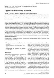
Figure 1: Two-phase adaptation and metrics for extinction avoidance and persistence. (a) Our scenario: shifting the mean environment (dashed to dotted vertical line) alters the mean optimum trait (from open circle to solid dot), while the change in environment autocorrelation changes the optimal plasticity (from slope of solid black line to that of dashed black line). Due to GxE, additive variance increases in the new environment (by a factor of approximately 9 for these parameters, grey band; see Discussion for empirical examples where such inflation may occur). During evolutionary rescue, the mean reaction norm (solid back line with slope initially evolved to match predictability ρ) increases transiently (grey line; note the intercept increases a small amount also) and eventually evolves to match the new predictability ρδ (slope of dashed black line). (b) Change occurs in two phases. Mean relative plasticity (¯b/B; versus time, log scale) increases quickly during Phase 1, then decays slowly during Phase 2. Over the transition from Phase 1 to Phase 2 (from tbef , dash vertical line, to taft , dash-dot vertical line), plasticity is relatively constant. (c) Population size versus time in simulations, mean size (grey line) declines during Phase 1 of rescue, while variance (thin lines) increases, heightening extinction risk. We compute the probability of quasi-extinction before rescue at tbef and at taft as the proportion of simulated trajectories below NC =100 (horizontal black bar). (d) The mean population growth rate (versus time, log scale) is initially negative, increases during Phase 1 and is relatively stable during Phase 2 (grey line). We define persistence as self-replacement after Phase 1, using growth rate predicted at the Phase’s end (solid horizontal line, r¯1 ≥ 0, eqn 3; note when accounting for both Phases, the growth rate slowly increase during Phase 2: grey line). Parameters: shift size δ = 4, predictability before ρ = 0.5 and after the shift ρδ = 0.4, selection strength ω 2 = 20, developmental delay τ = 0.2, additive genetic and environmental variances σa2 = 0.1, σb2 = 0.05, and σe2 = 0.5; initial population size N (0) = 104 , and maximum fitness ermax = 1.1.
21
shifted predictability (
ρ
0.75 0.50 0.25
0.3
+ 0.025 0.050 0.075 0.100
ρ = 0.7
+ 0.025 0.050 0.075 0.100
variance in plasticity (
2 ) b
shifted predictability (
+
0.75
+
0.04
0.50
-
0.25
2
3
4
0.00
5
6
2
3
4
-0.04 5
6
mean shift ( )
= 0.7
0.75 0.50 0.25
0.025 0.050 0.075 0.100
0.025 0.050 0.075 0.100 2 ) b
)
= 0.3
�
= 0.3
= 0.7
Simulated Pr(N < Nc)
0.75
0.75 0.50
0.50 0.25 0.25
2
3
4
5
6
2
3
4
5
6
0.00
mean shift ( )
= 0.3
= 0.7
0.75 0.50 0.25
0.025 0.050 0.075 0.100
0.025 0.050 0.075 0.100
variance in plasticity (
2 ) b
)
(f) �
shifted predictability (
(e) )
= 0.7 Growth rate
shifted predictability (
�
variance in plasticity (
shifted predictability (
= 0.3
(d)
)
(c)
�
shifted predictability (
�
)
(b)
)
(a)
�
= 0.3
= 0.7
Simulated Pr(Nt < Nc)
0.75
0.75 0.50
0.50 0.25 0.25
2
3
4
5
6
2
3
4
5
6
0.00
mean shift ( )
Figure 2: Potential for evolutionary rescue over a range of values for post-shift predictability ρδ versus genetic variance in plasticity the reference environment σb2 (a,c,e) and shift size δ (b,d,f). Within panels, columns show low (ρ = 0.3) and high (ρ = 0.7) initial predictability. (a,b) Growth rates at the end of rescue are computed from numerical simulations as the stochastic growth rate λs between tbef and taft spanning Phase 1 and 2 (diverging heatmap: white 0, blue positive, and red negative). Black lines indicate the threshold between decline (-) and persistence (+) based on the analytical approximation (¯ r1 = 0, eqn 3 ; solid line) and stochastic simulations (λs = 0, dotted black line). (c-f) Simulated probability of quasiextinction at a point during rescue (i.e, at tbef , (c-d) and total (i.e., up to taft , (e,f) darker colors indicate greater chance of extinction (grayscale heatmap). Quasi-extinction is the proportion of trajectories below a critical size NC by a given time (both at tbef or taft ; illustrated in Figure 1). When variance in plasticity is varied (a,c,e), shift size is set to δ = 4 (so that additive variance increases by a factor of 9 in the new environment when σb2 =0.05). When shift size is varied (b,d,f), variance is set to σb2 = 0.05. Other parameters: initial population size N (0) = 104 , selection strength ω 2 = 20, developmental delay τ = 0.2, additive genetic σa2 = 0.1 and environmental σe2 = 0.5 variances, maximum fitness ermax = 1.1, and variance in the environment σ 2 = 1.
22
Supplemental Information for “Predicting evolutionary rescue via evolving plasticity in stochastic environments” Jaime Ashander, Luis-Miguel Chevin, Marissa L. Baskett
Appendix A. Approximate dynamics of growth rate in terms of maladaptation x(t) Our equation (2) shows the Malthusian growth rate r(t) is the sum of the maximum Malthusian growth rate rmax , the variance load LG , and the lag load LL with rmax = log Wmax , LG = log and LL =
S(εc (t)) x(t)2 , 2
¯ (t) = rmax + LG (t) + LL (t). log W
�p
�
S(εc (t))ω 2 ,
(A.1)
Below, we derive an approximation to this where the only time dependence is through the squared maladaptation x(t)2 = (¯ z (t) − θ(εs (t)))2 . Appendix A.1. Strength of selection The strength of selection, S(εc (t)), appears in both the variance load LG and lag load LL but depends inversely on the phenotypic variance, which changes due to stochastic variation in the environmental cue, which affects the phenotype. Therefore, we approximate the expectation of the strength of selection using a Taylor series: � h
i
E[S(εc (t))] = E σz2 (εc (t)) + ω 2 � h
i
≈ E σz2 (εc (t)) + ω 2
�−1
�−1
−
Var(σz2 )3 Var(σz2 ) + O( ) 2E[σz2 ]3 E[σz2 ]4
.
Expanding σz2 using equation (1) of the main text and taking expectations, we get the approximate expected strength of selection Sδ , assuming δ ≪ σ 2 , which we denote �
Sδ = E[S(εc (t))] ≈ σa2 + σb2 (δ2 + σc2 ) + σe2 + ω 2
�−1
.
Where we use the E[εc (t)2 ] = Var[εc (t)] + E[εc ]2 and the mean environmental shift δ. Appendix A.2. Variance load The first term of equation (A.1) is the phenotypic variance load at time t LG (t) = 1/2 log S(εc (t)) + 1/2 log ω 2 . 1
(A.2)
Taking expectations, and using Taylor series: E[LG ] = 1/2 log ω 2 + 1/2E [log S(εc (t))] ≈ 1/2 log ω 2 + 1/2 log (E [S(εc (t))]) −
Var(σz2 ) 2E[σz2 ]2
≈ 1/2 log ω 2 + 1/2 log (E [S(εc (t))]) ≈ 1/2 log ω 2 + 1/2 log Sδ where the right hand side of the last line is the approximate expected variance load after using E [S(εc (t))] ≈ Sδ from (A.2). Appendix A.3. Lag load The second term of equation (A.1) is the lag load at time t, LL (t). Here we show that in expectation, this load has two components, a stochastic load and a shift load. To derive expressions for these, we take the expectation of the entire second term: S(εc (t)) x(t)2 , E[LL (t)] =E 2 � � � h � i S(εc (t)) S(εc (t)) , x(t)2 , =E E x(t)2 + Cov 2 2 �
�
where we used the identity Cov [ab] = E[ab] − E[a]E[b]. The covariance in the final line represents how stochastic changes in environment (and optimum) that cause maladaptation also cause either larger or smaller phenotypic variance, depending on the direction, due to our assumption that genetic variance in plasticity increases with δ. Furthermore, under weak stabilizing selection, variance in z contributes little to the strength of selection S. For both these reasons, we expect this covariance to be small. If we neglect the covariance term and use the approximate variance load from Appendix A.2 (Sδ in main text) the expectation is E[LL (t)] ≈ approximate the dynamics of the lag load
� Sδ � 2 2 E x(t) .
LL (t) =
Removing the expectation, we use this as to
Sδ x(t)2 . 2
Appendix A.4. Full dynamics Bringing together the approximations developed above, we have an expression for the growth rate, where all components except the maladaptation are averaged over the fluctuations, r(t) ≈ rmax + 1/2 log(ω 2 Sδ ) − 2
Sδ x(t)2 . 2
(A.3)
From this, we can obtain both the average long-run growth rate, by taking an expectation to obtain r¯(t) ≈ rmax + 1/2 log(ω 2 Sδ ) −
Sδ x(t)2 2 (¯
¯2 + σx2 ). This shows the lag load + σx2 (t)) (because E[x2 ] = x
consists of two loads. The first, expected load from reduction in log mean fitness due to maladaptation ¯(t)2 . of the mean trait relative to the mean optimum in the new environment, is “shift load” − S2δ x The second, expected load due to reduction in log mean fitness due to random fluctuations in the environment, is “stochastic load” − S2δ σx2 (t). We can also analyse the variance in trajectories of r(t), and thus population growth because log N (t + 1) = r(t) + log N (t). Both of our subsequent analyses require computing the dynamics of mean squared maladaptation x ¯(t)2 and the variance in maladaptation σx2 (t).
Appendix B. Dynamics of shift load depend on mean maladaptation x ¯(t)2 In this section, we derive the dynamics of the shift load − S2δ x ¯(t)2 under the approximation introduced by Lande [9] that separates adaptation into a fast Phase 1 and a slow Phase 2. We demonstrate that the population is approximately perfectly adapted in mean trait value by the end of Phase 1. We first write down the mean trait dynamics without the approximation, then describe the timescales of the two phase approximation, and derive approximate dynamics of the shift load owing to maladaptation in the mean trait.
Appendix B.1. Mean trait Trait dynamics follow the standard equation ∆y = Gβ, where y = (¯ a, ¯b)T , G is the additive genetic variance-covariance matrix, and β is the selection gradient. The selection gradient on reaction norm ¯ [from the equation for fitness above eq. (2) height and slope obtained by taking the log-gradient of W of main text; 9] is
β = −S(εc (t)) �
a ¯(t) − A + ¯b(t)εc − Bǫs �
a ¯(t) − A + ¯b(t)εc − Bǫs εc
.
(B.1)
With a constant additive genetic variance-covariance matrix (G matrix), the change per generation in a ¯(t) and ¯b(t) is given by
¯(t) a
∆
¯b(t)
2 σa
=
3
0
0
σb2
β.
In the new environment, the expectation of the change per generation conditional on a ¯ and ¯b is
a(t)) E(¯
∆
E(¯b(t))
= E[Gβ]
≈ −Sδ G
a ¯ − A + ¯bδ − Bδ E[(¯ a − A)εc (t)] + E[¯bε2c (t)] − BE[εc εs ]
,
where the approximation comes from the treating E[S(εc (t))] as a constant. We assume no environmental tracking by phenotypic plasticity, i.e., Cov[¯bt , εc (t)2 (t)] = 0 so E[¯bt ε2c ] = E[¯bt ]E[εc (t)2 (t)], or by reaction norm elevation, i.e., Cov[¯ at , εc (t)] = 0 so E[¯ at , εc (t)] = E[¯ at ]E[εc (t)]. Note that the tracking of the environment by the reaction norm elevation could be included, reducing the expected mean plasticity [28], but we neglect it here. However, we do allow for environmental tracking when computing the lag load (below). Then, using E[ε2 (t)] = δ2 + σ 2 and E[εc (t)εs ] = δ2 + ρσ 2 , the expectation of the change is approximately
E ∆
1
¯(t) a ¯b(t)
≈ −Sδ G
δ a ¯(t) − A
δ2
δ
¯b(t) − B
+
0
(¯b(t) −
ρB)σ 2
.
(B.2)
The approximation is exact if Cov[¯bt , εc (t)2 (t)] = Cov[¯ at , εc ] = 0. Note that this differs from Lande [9], where this relation was treated as exact [28]. We solve for the explicit trait dynamics relative to the long-run equilibrium state [9]. Setting selection gradient β in equation (B.1) to zero, solve for long run trait values
¯b∞
A + Bδ(1 − ρδ )
¯∞ a
=
Bρδ
(B.3)
˜ One can show, with some algebra [9], the one-generation change (B.2) is the product -Sδ Gz(t), where z(t) is the difference between mean trait values and their long-run equilibrium values computed above and
˜ = G
σa σb
2
2δ
σa σb
2 δ2
�
2δ
1+
σ2 δ2
� .
The expected dynamics can then be expressed in terms of the eigenvectors and eigenvalues of the matrix ˜ [9, 16], G z(t) = c1 e1 (1 − Sδ λ1 )t + c2 e2 (1 − Sδ λ2 )t ,
(B.4)
˜ respectively and ci terms are constants determined where ei and λi are eigenvectors and eigenvalues of G by initial conditions. 4
Appendix B.2. Approximation for a large environmental shift As in earlier work, we consider the case where the shift in the mean environment is very large relative to background noise,
σ2 δ2
˜ ≪ 1. Here, we initially write down the eigenvalues and eigenvectors of G
to first order in this small term, but thereafter follow Chevin and Lande [16] in deriving approximate dynamics to leading order. To first order in
σ2 δ2
σa2
λ1 =
λ2
and the eigenvectors are
�
δ (1 − φ) 1 −
e1 =
, the eigenvalues are +
δ2 σb2 σ
φ
+
2 σ2 a δ2
� ,
σ2 φ δ2
�
2 δ2 σb2 σδ2 φ
,
φ
�
δ 1+
e2 =
� .
σ2 φ δ2
−1
These match the calculations of [9] up to a constant of Sδ (equivalent to γ in Lande [9]). Assuming the population has long evolved in an environment with predictability ρ, the initial trait values are (¯ a0 , ¯b0 ) = (A, ρB). Using (B.3), the initial conditions in the re-centred trait x are
−Bδ(1 − ρδ )
z0 =
To leading order, the constants are
c1
c2
=
B(ρ − ρδ )
−B(1 − ρ) −B(ρ(1 − φ) − ρδ + φ)
Appendix B.2.1. Timescales of phases 1 and 2 If most phenotypic variation in the new environment is due to variance in plasticity, φ ≈ 1, and the shift in the mean environment is large (relative to background variability as in our approximation above), the trait change takes place in two phases that occur at very different timescales [9]. When selection is weak, geometric terms in (B.4) can be replaced by exponential terms e−tSδ λi , indicating the relative timescales of change along the eigenvectors ei are given by ti ≈
1 λi .
2
The ratio t1 /t2 ≈ φ(1 − φ) σδ2 , and
when much of the additive genetic variation is due to variation in plasticity so φ ≈ 1, then t1 /t2 ≈
σ2 , δ2
which is small in the approximate case we treat. Then, change along e1 occurs very fast relative to change along e2 [9]. At the end of Phase 1, e−tSδ λ1 ≈ 0 while e−tSδ λ2 ≈ 1 Thus, the approximate state 5
of the system relative to its final state, i.e., (B.3), is c2 e2 . The trait values, at the end of Phase 1 are, to leading order,
¯O(t1 ) a
E
¯bO(t ) 1
A + Bδ(1 − ρ)(1 − φ)
≈
(B.5)
B(ρ + φ(1 − ρ))
The effect of the initial environment occurs through predictability ρ, which under our assumption that the population is adapted initially also determines the initial mean plasticity ¯b0 = ρB. We see the initial plasticity has a strong influence at the end of Phase 1 only if φ is small. When φ is large, the plasticity at the end of Phase 1 is close to “perfect” i.e. bO(t1 ) ≈ B. Note also that to first order, the mean phenotype is perfectly adapted z¯O(t1 ) ≈ A + Bδ. Where the extinction risk is calculated at half of the characteristic timescale of Phase 2, i.e., tbef =
φδ2 2σa2 σ2
Appendix B.2.2. Trait dynamics during Phase 1 Throughout Phase 1, the term (1 − Sδ λ2 )t ≈ 1, so the dynamics are given by z(t) = c2 e2 + c1 e1 (1 − Sδ λ1 )t . We again replace the geometric term with an exponential (valid for weak selection) and re-normalize. To leading order, after some rearranging, the right hand side of the expected dynamics is
¯(t) δ(1 − φ) A a −tS λ , + = 1 − e δ 1 B(1 − ρ)
E
¯b(t)
�
�
φ
Bρ
(B.6)
which is analogous to the result of Chevin and Lande [Supporting Information, eq A6; 16]. As in that paper, we compute the eigenvalue only to leading order in the expression
σa2 1−φ
σ2 δ2
so λ1 ≈ σa2 + δ2 σb2 which is equivalent to
used in Chevin and Lande [16].
Appendix B.2.3. Trait dynamics during Phase 2 During Phase 2, the term (1 − Sδ λ1 )t ≈ 0, so the dynamics are given by z(t) = c2 e2 (1 − Sδ λ2 )t . Then, using (B.3) and again replacing the geometric term with an exponential (valid for weak selection) and re-normalizing, the expected dynamics to leading order in
σ2 δ2
during Phase 2 are
2 ¯(t) A + Bδ(1 − ρδ ) δ −tSδ σa2 σδ2 φ a , e − B(ρ − ρδ + φ(1 − ρ)) =
E
¯b(t)
Bρδ
6
−1
(B.7)
2
where we have used λ2 ≈ σa2 σδ2 φ. Note that for t = O(t1 ), this exponential term equals 1 and this equation agrees with (B.5).
Appendix B.3. Dynamics of expected maladaptation during Phase 1 We derive the expected maladaptation of the mean trait during an initial phase of evolutionary rescue, focusing on a case where the size of the environmental shift is large and much of the additive genetic variance in the new environment owes to genetic variance in reaction norm slope. The shift load (computed in Appendix A) is
Sδ ¯(t)2 . 2 x
After we compute the dynamics of the mean maladaptation
x ¯(t)2 , we will have an approximation for dynamics of the shift load, �
�2
x ¯(t)2 = E[x(t)]2 = E[¯ a(t)] − A + E[¯b(t)εc (t)] − BE[εs ] �2
�
≈ E[¯ a(t)] − A + δ(E[¯b(t)] − B)
.
The last equation comes from assuming the covariance between reaction norm slope and the cuing environment is small relative to the mean value of the new environment. Then, E[¯b(t)εc (t)] ≈ E[¯b(t)]E[εc (t)] = δE[¯b(t)] in the new environment. This is reasonable when
σ2 δ2
≪ 1. After using (B.6)
and some algebra, we obtain 2 σa
x ¯(t)2 ≈ B 2 δ2 (1 − ρ)2 e−2tSδ 1−φ .
(B.8)
Where we use φ to represent the proportion of additive genetic variation in the new environment due to variation in plasticity, φ=
δ2 σb2 . σa2 + δ2 σb2
Equation (B.8) indicates the shift load goes to zero as t increases.
Appendix C. Stochastic load: variance in maladaptation σx2 at stationarity Appendix C.1. Perceived environment with fixed plasticity A tactic from Michel et al. [35] aids in calculating the variance as a function of fixed plasticity. We define the perceived optimum ψ(t) as the difference between the optimum and the mean trait after accounting for the plastic response ψ(t) = Bεs (t) − ¯b∗ εc (t) so that x(t) = a ¯(t) − ψ(t). Then, the perceived variance in the optimum is σψ2 (¯b∗ , ρδ ) = σ 2 (B 2 + ¯b∗ (¯b∗ − 2Bρδ )), 7
(C.1)
and autocorrelation in the perceived optimum is "
1/τ Tψ (¯b∗ , ρδ ) = − log ρδ
B¯b∗ (ρ−1 δ − ρδ ) 1− 2 ∗ ¯ ¯ B + b (b∗ − 2Bρδ )
!#−1
(C.2)
[35]. We can then express maladaptation in terms of the intercept and perceived environment as x(t) = a ¯(t) − ψ(t). Appendix C.2. Variance at stationarity We derive an approximation for variance in maladaptation under stationarity, which we denote σx2 . In practice, this means we solve for the effect of fluctuations on maladaptation after a long time, we assume the mean maladaptation is zero, and we also assume fixed mean plasticity ¯b∗ . We are interested in finding an asymptotic expression for the variance of this term. Assuming fixed plasticity, all change in the trait occurs through change in the reaction norm height, ∆¯ z = ∆¯ a(t) = −Sδ σa2 x(t). When selection is weak relative to genetic variance in reaction norm height, and the fluctuations in the perceived environment are not large, evolution can be approximated in continuous time [22, 35] as dψ dx + Sδ σa2 x = − , dt dt where x = a ¯(t) − ψ. For t ≫ t1 and constant genetic variance σa2 , the solution to this differential equation is a ¯(t) = Sδ σa2
Z
∞
0
�
�
exp −Sδ σa2 τ ψ(t − τ )dτ.
(C.3)
What remains is to compute Var[x(t)]. Using our quasi-stationarity assumption, we need only compute E[x(t)2 ] = −2E[¯ a(t)ψ(t)] + E[¯ a(t)2 ] + E[ψ(t)2 ]. The last of these expectations is simply the variance of the perceived environment σψ2 . The first and second expectations integrate over time (from eq. C.3), −2E[¯ a(t)ψ(t)] = −2Sδ σa2 2
E[¯ a(t) ] =
Sδ2 σa4
Z
0
Z
∞
�
�
exp −Sδ σa2 τ E[ψ(t)ψ(t − τ )]dτ
0 ∞Z ∞ 0
�
�
exp −Sδ σa2 (τ1 + τ2 ) E[ψ(t − τ1 )ψ(t − τ2 )]dτ1 dτ2 .
Because ψ is a linear combination of autoregressive Gaussian processes εc (t) and εs , we can express the expectations involving ψ in terms of autocovariance E[ψ(t), ψ(t − τ )] = σψ2 exp(−τ /Tψ ) and E[ψ(t − τ1 ), ψ(t − τ2 )] = σψ2 exp(−|τ1 − τ2 |/Tψ ). In both of these expressions, Tψ is the characteristic autocorrelation time of the perceived environment ψ. 8
The first expectation is −2E[¯ a(t)ψ(t)] =
−2Sδ σa2 σψ2
∞
Z
0
�
�
exp −τ (Sδ σa2 + 1/Tψ ) dτ,
Tψ Sδ σa2 σψ2 . = −2 (Tψ Sδ σa2 + 1)
The second expectation involves an absolute value term, meaning the integral must be taken in two parts, and evaluates to E[¯ a(t)2 ] =Sδ2 σa4
Z
0
=Sδ σa2 σψ2
∞Z ∞ 0
�
�
exp −Sδ σa2 (τ1 + τ2 ) σψ2 exp(−|τ1 − τ2 |/Tψ )dτ1 dτ2 ,
Tψ (Tψ Sδ σa2 + 1)
Combining these expressions, 2
E[(¯ a(t) − ψ(t)) ] =
σψ2
!
Tψ Tψ Sδ σa2 + Sδ σa2 +1 −2 2 (Tψ Sδ σa + 1) (Tψ Sδ σa2 + 1)
� � σψ2 2 2 2 = T S σ + 1 − 2T S σ + T S σ ψ δ ψ δ ψ δ a a a (Tψ Sδ σa2 + 1)
σx2 (¯b∗ , δ, ρδ ) :=
σψ2 , (Tψ Sδ σa2 + 1)
where the last line defines the variance we sought to calculate. As our notation emphasizes, this load depends primarily on the level of plasticity ¯b∗ and the size of the shift δ. Note that this formula matches Lande and Shannon [22].
Appendix C.3. Quasi-stationary variance over Phase 1 The variance in maladaptation σx2 depends on variance σψ2 (¯b∗ , ρδ ) from eq. (C.1) and characteristic timescale Tψ (¯b∗ , ρδ ) from eq. (C.2) of perceived fluctuations in the perceived optimum (given autocorrelation ρδ at timescale τ in the true optimum), as σψ2 (¯b∗ , ρδ ) �. σx2 (¯b∗ , δ, ρδ ) = � Sδ σa2 Tψ (¯b∗ , ρδ ) + 1
(C.4)
After a long time, on the timescale of Phase 1, t1 , the mean maladaptation is zero, as shown in eq. (B.8), and the variance in maladaptation is stationary. At this point, as shown in Appendix B, plasticity is at its approximate maximum bmax = B(ρ + φ(1 − ρ)). It remains as this value for a long time (on the scale of Phase 1; although eventually decays to the predictability ρδ according to the dynamics in Appendix 9
B.2.3) and so we evaluate (C.4) at bmax to determine persistence in (3). Using the “quasi-stationary” approximation that fluctuations achieve stationarity while ¯b∗ = bmax , we evaluate σx2 (bmax , δ, ρδ ). Note that we could also evaluate (C.4) at any time t during Phase 1, σx2 (t) = σx2 (¯b(t), δ, ρδ ),
(C.5)
by using dynamics for reaction norm slope ¯b(t) from eq. (B.6). Doing so assumes for each change in ¯b over Phase 1 the stochastic variance in maladaptation achieves stationarity. No doubt this is inaccurate in some cases, but it is a tractable analytical approximation for the variance. Using this approximation over the parameter ranges we examine in this paper, the stochastic load does not change much with changes in plasticity (Figure S1). Accordingly, we use the simpler approximation above, and evaluate the variance at bmax for all time.
Appendix D. Simulation In simulation, we implement the autocorrelated environment as an autoregressive function with correlation κ on a timescale with n = ceiling[ τ1 ] time units in a generation. The process simulated is xi = κxi−1 +
p
1 − κ2 ξσ,
where ξ is a unit normal random variable. If x and ξ are independent (as generally assumed in autoregressive functions) and the process is stationary, it has variance σ 2 (and mean 0). Further, the covariance of observations one time unit apart is κσ 2 and the correlation of such pairs of observations is κ. For observations n time units apart, the correlation becomes κn . Thus, using the n time steps per generation, the simulated process relates to the exponential autocovariance function given above as κn = ρ1/τ . Accordingly we set the correlation within simulations equal to that of the environmental predictability at timescale τ , i.e., κ = ρ.
Appendix E. Alternative assumptions of reaction norm shape If, instead of assuming phenotypic variance in the reference environment is minimal, we assume the environment is shifted to an environment where the variance is minimal, then the additive genetic variance of the expressed trait z(t) increases quadratically away from the novel environment εc (t) = δ. Without the assumption that variance is minimized in the reference environment, the additive genetic 10
covariance between a and b is non-zero in the reference environment [9]. From that paper, the full form of (1b) is σz2 (εc (t)) = σa2 + 2σab εc (t) + σb2 ε2c (t) + σe2 , where σab is the additive genetic covariance between reaction norm slope and variance in the reference environment. (With the assumption of variance minimized at εc = 0, σab = 0, and the covariance in any other environment is Cov(a, b) = σb2 εc .) Then σz2 (εc (t)) is minimized in the environment ε∗c = −σab /σb2 [9]. Thus, assuming minimal variance in the new environment implies σab = −δσb2 . The mean of the expressed trait value z(t) before selection is the same as in (1), but the variance differs, giving z¯(t) = a ¯(t) + ¯b(t)εc (t)
(E.1a)
σz2 (εc (t)) = σa2 − 2σb2 δεc (t) + σb2 ε2c (t) + σe2 ,
(E.1b)
which assumes the additive genetic variances are constant in time. In this case, the expressed trait z and the slope b have covariance Cov(z, b) = (εc (t) − δ)σb2 and so, with εc (t) ≈ δ there is approximately zero covariance between the trait and reaction norm slope, and so direct selection on the trait results in very weak selection on reaction norm slope. Consequently, the transient increase in plasticity should not be expected without the assumed increase of genetic variance in novel environments. Given the uncertainty described by McGuigan and Sgro [12] concerning the effects of stress (i.e., novelty) on additive genetic variance, theory could usefully outline empirical possibilities. The derivation of (E.1) is just the beginning. It does show, however, that the theory presented in the main text is not completely general. No theory is unless it thoroughly considers the possible relationships between additive genetic variance and environmental shifts. In the main text, we analyse only one set—where many are possible—of assumptions on how plasticity, demography, and evolution interact during evolutionary rescue. However, this set of assumptions appears met by empirical reality in at least some cases (see main text, "Assumptions and Caveats").
Appendix F. A small shift and large additive variance in plasticity σb2 We expect our approximation to perform best when a large proportion of additive variance in the novel environment is due to variance plasticity (i.e., φ ≈ 1). This occurs in our model either when σb2 (GxE) is large in the reference environment, or when a large shift in the mean environment causes quadratic increases in additive genetic variance (as δ2 σb2 ). In the former case, the population has inherently high genetic variability in plasticity, and our assumptions imply a relatively large changes in additive genetic variance for even small shifts in the mean 11
environment. In the latter case, increased additive genetic variance is driven by the novelty of the environment. Simulations reveal that despite both cases increasing φ, the approximation does not perform equivalently well. If the mean shift is small then the approximation for the threshold between decline and persistence performs poorly as additive variance in plasticity increases (δ = 1.5, Figure S5). In fact, the approximation appears to perform better for lower values of φ.
15
20
25
30
5
60
80
100
0
100
200
300
time
time
time
δ = 3 ρ δ = 0.5
δ = 6 ρ δ = 0.5
10
15
20
25
30
0.20 0.15 0.10 0.05 0.00 0
20
40
60
80
100
0.20 0.15 0.10 0.05 0.00 0
100
200
300
time
time
time
δ = 1 ρ δ = 0.75
δ = 3 ρ δ = 0.75
δ = 6 ρ δ = 0.75
0.20 0.15 0.10 0.05 0.00 0
40
stochastic load
5
20
δ = 6 ρ δ = 0.25 0.20 0.15 0.10 0.05 0.00
δ = 1 ρ δ = 0.5 0.20 0.15 0.10 0.05 0.00 0
0
stochastic load
10
δ = 3 ρ δ = 0.25 0.20 0.15 0.10 0.05 0.00
10
15
20
25
30
0.20 0.15 0.10 0.05 0.00 0
20
40
time
60 time
80
100
stochastic load
5
stochastic load
0
stochastic load
δ = 1 ρ δ = 0.25 0.20 0.15 0.10 0.05 0.00
stochastic load
stochastic load
stochastic load
stochastic load
Appendix G. Supplementary Figures
0.20 0.15 0.10 0.05 0.00 0
100
200
300
time
Figure S1: Quasi-stationary stochastic load plotted against time during Phase 1 (up to the characteristic timescale of Phase 2 t2 ) for the same values of relative plasticity α as Figure S2. While changes in the magnitude of stochastic load over Phase 1 are not large, and in some cases not apparent, when the change reduces (or increases) the mismatch the ˜ stochastic load follows (e.g., bottom right or top right panel). Other parameters are σb2 =0.05, S(δ) =0.0446429, B =2, σ 2 = 1, σa2 =0.1.
12
δ =3
δ
0.10 0.05
0.20 stochastic load with plasticity
0.15
0.00
0.15 0.10 0.05 0.00
0.2
0.4
0.6
0.8
1.0
00
02
δ =1
0.3 0.7
0.05
0.
0.8
1.0
0.0
0.2
0.4
0.15
0.10
0.1
0.05 0.00 0.6
0.8
stochastic load without plasticity
0.15
0.15
0.55
0.10
0.1
0.05 0.00 0.0
0.2
0.4
ρδ
0.8
1.0
=6 ^2 σ a
0.20
1.0
0.6 ρδ
δ =3 2
σa
0.4
0.1
0.10
ρδ
0.20
0.
06
04
ρδ
0.0
α
0.15
0.00
0.6
0.8
1.0
ρδ
stochastic load without plasticity
0.0
stochastic load without plasticity
δ =6
0.20 stochastic load with plasticity
stochastic load
0.20
^2
0.20
a
0.15
1.9
0.10
0.1
0.05 0.00 0.0
0.2
0.4
0.6
0.8
1.0
�
Figure S2: Top row: Stochastic load with plasticity plotted against ρδ for various values of relative plasticity α. Bottom row: Stochastic load without plasticity (i.e., load component for “positively auto-correlated fluctuations" from Table 1 of Lande and Shannon 1996) plotted against ρδ for equivalent values of total additive genetic variance. Specifically, the additive genetic variance in reaction norm elevation is adjusted to value σ ˆa2 , set either to its intial value (ˆ σa2 = σa2 , grey line) or to the total additive genetic variance in the new environment with plasticity in the top row (ˆ σa2 = δ 2 σb2 + σa2 , black line). ˜ Also, note that relative plasticity α has no effect in the bottom row). Other parameters are σb2 =0.05, S(δ) =0.0446429, B =2, σ 2 = 1, σa2 =0.1.
0.10 1
variance load
0.08
2 3 0.06
4 5
0.04
6
0.02 0.00
0.04
0.08 2
Figure S3: Variance load plotted against σb2 for various values of δ. Other parameters are B =2, σ 2 = 1, σa2 =0.1. Note predictability after shift ρδ does not affect variance load.
13
growth rate (log W)
0.0 0.2 0.4 0.6
10
1000
10
1000
10
1000
10
1000
time (generations)
population size (N)
D
E
F
10000
100
10
1000
10
1000
time (generations)
¯ , A-C), and population size (log N , D-F) versus time (in generations, log scale) Figure S4: Dynamics of growth rate (log W under evolutionary rescue for three scenarios of environmental shift δ and predictability ρδ following the shift: a modest shift and low predictability (δ =2.5, ρδ =0.3: A,D), a modest shift and high predictability (δ =2.5, ρδ =0.7: B,E), and a large shift and high predictability (δ =5, ρδ =0.7: C,F). Each panel shows 10 replicate simulations of 1500 generations (thin black lines), the mean of these simulations (thick grey line), and predicted trajectories of the mean (solid black line); also shown for comparison are predictions without amplifying effect of plasticity on stochastic fluctuations (dash-dot line). The dashed vertical lines indicate the time during Phase 1 at which we compute quasi-extinction before rescue (tbef ; see Figure 1). Parameters: initial predictability ρ = 0.5, additive genetic variance in plasticity σb2 = 0.05; other parameters as in Figure 2. Greater shift size implies larger increase of additive genetic variance in the new environment; for a modest shift (A,B, D,E) our model assumes additive genetic variance increases by a factor of 4, for a large shift, (C,F) the increase is by a factor of 14.
14
) shifted predictability (
= 0.
= 0.
0. 5
0.04
0.50
0.00
0.25
-0.04
0.0250.0500.0 50.100 0.0250.0500.0 50.100
shifted predictability (
)
variance in plasticity (
= 0.3
2 ) b
= 0.7
imulate r(N N ) 0.75
0.75
0.50 0.50
0.25
0.25
0.0250.0500.0750.100 0.0250.0500.0750.100
)
variance in plasticity (
shifted predictability (
Growth rate
= 0.3
0.00
2 ) b
= 0.7
imulate r(Nt N ) 0.75
0.75
0.50 0.50
0.25
0.25
0.0250.0500.0750.100 0.0250.0500.0750.100
variance in plasticity (
0.00
2 ) b
Figure S5: Potential for evolutionary rescue over a range of values for post-shift predictability ρδ versus genetic variance in plasticity the reference environment σb2 (A,B). Within panels, columns show low (ρ = 0.3) and high (ρ = 0.7) initial predictability. A Growth rates at the end of rescue are computed from numerical simulations as the stochastic growth rate λs between tbef and taft spanning Phase 1 and 2 (diverging heatmap: white 0, blue positive, and red negative). Black lines indicate the threshold between decline (-) and persistence (+) based on the analytical approximation (¯ r1 = 0, eqn 3 ; solid line) and stochastic simulations (λs = 0, dotted black line). B Simulated probability of quasi-extinction before rescue. Quasi-extinction is defined at tbef as illustrated in Figure 1. Shift size is set to δ = 2.5 (so that additive variance increases by a factor of 4 in the new environment when σb2 =0.05). Other parameters: initial population size N (0) = 104 , selection strength ω 2 = 20, developmental delay τ = 0.2, additive genetic σa2 = 0.1 and environmental σe2 = 0.5 variances, and maximum fitness ermax = 1.1.
15
0.25
0.025
0.050
0.0 5
0.25
E
0.075
0.100
2.0
2.5
0.25
0.075
variance in plasticity (
-0.04
3.0
3.5
4.0
= 0.7 imulate r(N N ) 1.00
0.75
0.75 0.50
0.50
0.25 0.25
1.5
2.0
2.5
3.0
3.5
4.0
0.00
= 0.7
)
)
1.5
F
0.50
Figure S6:
-
mean shift ( )
0.75
0.050
0.25
2 ) b
= 0.7
0.025
0.00
)
0.50
variance in plasticity (
0.04
0.50
D
0.75
0.050
+
0.75
mean shift ( )
shifted predictability (
) shifted predictability (
0.100
Growth rate
2 ) b
= 0.7
0.025
= 0.7
)
0.50
variance in plasticity (
shifted predictability (
shifted predictability (
0. 5
0.100
shifted predictability (
) shifted predictability (
B
= 0.
imulate r(Nt N ) 0.75
0.75 0.50
0.50 0.25 0.25
1.5
2 ) b
2.0
2.5
3.0
3.5
4.0
0.00
mean shift ( )
Figure 2 but with genetic variance changing with population size according to a modified Stochastic House
of Cards (SHC) approximation: σSHC (σg2 ) = σg2 /(1 +
2 ω 2 +σe ) µ2 Ne
and Ne ≈ 2R0 N/(2R0 − 1). Parameters and panels are as
2
in Figure 2 with the additional parameter µ , which is the variance of the effect of new mutations, fixed at µ2 = 0.005. For the un-modified SHC the numerator, σg2 , is replaced by a term that includes the per-generation total mutation rate Vm and the strength of selection: 2Vm (ω 2 + σe2 ) [see 23, who used α2 instead of µ2 ]. Thus, the modified version we use effectively assumes that larger initial values of σa2 and σb2 reflect populations with larger mutation rates.
16