Predicting Future Locations Using Prediction-by-Partial-Match Ingrid Burbey
Thomas L. Martin
Virginia Tech, Dept. of ECE 302 Whittemore Hall, 0111 Blacksburg, VA 24061
Virginia Tech, Dept. of ECE 302 Whittemore Hall, 0111 Blacksburg, VA 24061
[email protected]
[email protected] predict our future location: a smart reminder system, a locationsensitive to-do list, a connectivity predictor, or a smart home that adapts its environment to our activities. When the prediction information is shared with other people, other services become possible, such as serendipitous meetings or the exchange of favors [2]. Our goal in this research project is to expand upon the stateof-the art in location prediction by predicting future locations, not just the next location.
ABSTRACT We implemented the Prediction-by-Partial-Match data compression algorithm as a predictor of future locations. Positioning was done using IEEE 802.11 wireless access logs. Several experiments were run to determine how to divide the data for training and testing and how to best represent the data as a string of symbols. Our test data consisted of 198 datasets containing over 28,000 pairs, obtained from the UCSD Wireless Topology Discovery project. Tests of a first-order PPM model revealed a 90% success rate in predicting a user’s location given the time. The third-order model, which is given the previous time and location and asked to predict the location at a given time, is correct 92% of the time.
Current state-of-the-art in location prediction predicts where someone will go next, as shown in the research projects listed in section 2. In addition to questions like “Where will Bob go next?” we would like to be able to answer questions such as “Where will Bob be at 10:30 a.m. this morning?” or “When will Bob next be in the office?” The experiments performed for this paper focus on using data compression to answer questions like “Where will Bob be at a given time?”
Categories and Subject Descriptors I.6.5 [Simulation and Modeling]: Model Development – Modeling methodologies.
General Terms
Previous research in location prediction represents a sequence of locations as a series of alphanumeric characters and uses algorithms based on probabilistic techniques such as Markov models to predict the next character in the sequence. These probabilistic algorithms are the same algorithms used to create efficient data compressors. Efficient data compressors make good sequence predictors.
Algorithms, Design, Experimentation.
Keywords Prediction, supervised positioning.
learning,
data
compression,
WiFi
1. INTRODUCTION In the short story “What You Need” in the October 1945 issue of Astounding Science Fiction, author Lewis Padgett explores the life of an Electrical Engineer who has built a machine that predicts pivotal moments in people’s lives [1]. While such a prediction machine is still a flight of fancy, simply being able to predict where a person is likely to be can be useful for many pervasive computing applications. The project described in this paper predicts people’s future locations using a data compression technique called Prediction-by-Partial-Match (PPM).
We are interested in expanding the state-of-the-art to predict future locations, by transforming the prediction problem from a single-dimension, that of location, to multiple dimensions, that of location, time and potentially other useful indicators of context.
2. PREVIOUS WORK Predicting the next item in a sequence has been done for many domains, including branch prediction in microprocessors [3], instruction prefetch [4] and prediction of web pages to be requested [5]. But the area of research closest to the topic of this paper is predicting the next location in order to support contextawareness. The remainder of this section provides a brief overview of this research.
Our location is a key indicator of our context and likely indicates our current activities. A system that can predict our future locations can proactively adapt to our needs, turn lights on before we enter a room, or remind us of things we may need in the near future. One can easily imagine many uses for a system that can
The MavHome at the University of Texas in Arlington is an excellent example of location prediction used to improve the inhabitants’ lives and to reduce operating expenses [6]. The MavHome is divided into zones; each of which is labeled by an alphabetic character. Someone’s movement through the home is then recorded as a sequence of letters, such as mamcmr. Initially, prediction of the next character in the sequence was used to reduce the number of motion sensors which needed to be polled in order to ‘find’ the inhabitant in the home. Later, the prediction of
Permission to make digital or hard copies of all or part of this work for personal or classroom use is granted without fee provided that copies are not made or distributed for profit or commercial advantage and that copies bear this notice and the full citation on the first page. To copy otherwise, or republish, to post on servers or to redistribute to lists, requires prior specific permission and/or a fee. MELT’08, September 19, 2008, San Francisco, California, USA. Copyright 2008 ACM 978-1-60558-189-7/08/09...$5.00.
1
the inhabitant’s location was used to turned on lights and heating before the inhabitant entered a room or to allocate network resources in advance [7]. Prediction is done using a modified version of the Lempel-Ziv compression algorithm [8], which allows the researchers to predict segments of an inhabitant’s path through the house. The MavHome is a limited space with specialized sensors, and the research was done on a small number of people. In contrast, our goal is to apply prediction to a larger number of users using a globally available positioning system over a larger area.
a sequence q1n = q1q2 q3 L qn , where q i ∈ Σ . Given a test sequence x0T = x0 x2 L xT , the average log-loss l ( Pˆ , x0T ) is given by
1⎡T ⎤ l ( Pˆ , x0T ) = − ⎢∑ log 2 Pˆ ( xi | x0 x1 L xi −1 ) + log 2 Pˆ ( x0 )⎥ T ⎣ i =1 ⎦ The log-loss equation relates to the number of bits required to compress a string. Minimizing the average log-loss corresponds to maximizing the probability assignment for the test sequence. This average log-loss equation will be used later in section 3.3 to determine how to subdivide the data for training and testing.
Ashbrook and Starner collected GPS readings from several users over several months and used clustering techniques to extract the most significant locations from the large collection of data. A Markov model was then used to predict the users’ next significant locations [2, 9]. This project did not attempt to predict the route taken between the users significant locations. It predicted the user’s next destination, not how the user was going to get there. Our future goals include predicting paths of movement.
Begleiter’s results found that the Context-Tree-Weighting (CTW) and Prediction-by-Partial-Match (PPM) algorithms performed the best for music prediction. The CTW algorithm is very resourceexpensive, using a large amount of memory, so we focused on using the PPM algorithm to predict future locations.
3. METHOD We used wireless data traces from an IEEE 802.11 wireless network at the University of California San Diego [15] as the source of our location data. This data was filtered and mined to reproduce users’ paths. Portions of the data were used for supervised learning, i.e., to train the model, and the remaining data were used to test the effectiveness of the training model. The Prediction-by-Partial-Match data compression algorithm was used as the basis for our model. The details of each of these steps are given in the following sections.
Both of these projects studied a small group of users in a limited environment or time period. One of our objectives is to develop a prediction system using a larger group of users in a larger space, such as students on a college campus, using a readily available location system that works both indoors and outdoors A massive study at Dartmouth College applied several prediction techniques to wireless traces of over 6,000 users collected over a two-year period [10]. Prediction of the next IEEE 802.11 access point association is another method of location prediction because access points can be used as location beacons [11]. The Dartmouth study compared Markov predictors with Lempel-Ziv based predictors and found that low-order Markov models with a fallback scheme performed as well as the other algorithms over long historical traces. The second order Markov model with fallback achieved prediction success rates of 65 – 72 %. Our objective is to add temporal information to improve the predictions and predict future locations.
3.1 The Prediction-by-Partial-Match Algorithm The Prediction by Partial Match (PPM) algorithm is a variableorder Markov Model which uses various lengths of previous contexts to build the predictive model [16]. A table is built for each order, from 0 to the maximum order of the model. The training string is parsed into sub-strings. The context for each substring is the character(s) that precede the sub-string. Counters in each table keep count of how often each substring has been encountered in the given context. An articulate example of using the PPM model for prediction is given in [17].
The Rhythm Awareness Project by Hill and Begole [12, 13] is an interesting work that predicted times when work associates would be online. A predictor of when people are online is also a predictor of when they are in the office. This awareness is useful for knowing when co-workers may be available for a meeting or an impromptu phone call.
When the PPM model is queried, it searches the highest-order table for the given context (the preceding characters). If the context is found, the following character with the highest count is returned as the likely prediction. If the given context does not match any entries in the table, the context is shortened by one character and the next lowest-order table is searched. This process is repeated until the context is matched or the zeroth order table is reached. The zeroth order table simply returns the most common character seen in the training string.
Each of the preceding works predicts one dimension – either location or time. Our eventual goal is to be able to predict both: someone’s location at a future time. One issue is how to represent different types of data (in our case, location and time) in a text string. Begleiter et al. [14] compared several different variableorder Markov models on several different problems to see which was the best predictor. One of their datasets included music. Musical notation has much in common with the temporal and location data that we would like to model. The musical notation used by Begleiter includes notes, their starting times and duration, which is similar to our location sequences which include locations, and the starting times and duration spent at those locations. The musical information was represented by a string of interval values for the note, starting time and duration, separated by a colon. Prediction performance was measured using the average log-loss. Given an alphabet Σ , an algorithm is trained on
3.2 Location Data The first step in the prediction process is determining and recording past locations in order to predict future locations. Any positioning system can be used as long as it supplies enough information to determine the users’ symbolic locations and includes the temporal information such as when the user arrived at each location and how long he stayed. Any positioning system would require filtering to remove noise, data mining to extract significant locations and translating positions to symbolic locations (places). While the implementation of these steps may
2
be different for each positioning system selected, the general result is that any positioning system could be used for prediction.
Average of Average Log-Loss for PPM for Various Combinations of Training and Testing Weeks 6
Average of Average Log-Loss (PPM Model)
In this project, location was determined using nearby IEEE 802.11 wireless access points as location beacons. The advantages of this technique are that wireless access points are pervasive throughout a campus environment and can be sensed both indoors and outdoors. The location can be calculated on the user’s device, which supports the user’s privacy. One disadvantage of using wireless access points for positioning is the lack of a coordinate system, which is needed to triangulate position between multiple access points and to determine which access points are close together and could possibly be clustered together. Another difficult problem that arises with both GPS and WiFi positioning systems is that of translating positions into meaningful places. Any useful application needs to report location in the terms we use every day: office, home, lab, Burger King.
5
4
3
2
1
0 1-1
1-2
1-3
1-4
1-5
2-5
3-5
4-5
5-5
1-1
1-2
1-3
1-4
6
1-5
4-9
5-9
6-9
7-9
8-9
9-9
10
Weeks used for Training/Week used for Testing
Figure 1. Average Log-Loss for Different Training and Testing Schemes (for sequences containing only locations)
We used data from the Wireless Topology Discovery (WTD) project at UCSD for our experiments. In this project, researchers issued PDAs to 300 freshmen and collected movement traces [15]. The resulting dataset consists of two files: one file containing the access point locations and one file with trace data. The data were collected during an eleven week period from 9/22/2002 to 12/8/2002.
4. Representations of the Data While it is straight-forward to represent a series of locations as a sequence of alphanumeric characters, there are several different ways to represent both the temporal and location information. Our next set of experiments revealed that the choice of representation can make a significant difference in the ability of the model to predict future locations.
3.3 Subdividing for Training and Testing
The records in the dataset consist of the date followed by several tuples of (starting time, location, duration). These records need to be translated into character strings to train and test the PPM model. Because there are so many possible values for starting times, locations and durations, the original model code (based on [18]) was expanded to use 16-bit symbols instead of 8-bit characters.
Predictive models are trained on a subset of the data and then queried to predict some test data that are not known to the model. So the first step in developing any of the predictive models is to divide the training data into two parts: the portions used for training and the portions used for testing. Average log-loss, used by Begleiter to compare algorithms, was used to compare prediction success with varying weeks of training data. The code used by Begleiter, Java-based with a MATLAB wrapper, is available online [14] and was used for this portion of our experiment.
There is a balance to be considered when determining the representation of the data. A representation which adds some useful redundancy [19] may make patterns easier to discover. However, these representations increase the alphabet size of the model, thus making the model larger and less accurate because there are more choices for each prediction. On the other hand, a more concise representation may result in a smaller model, which may not find common patterns.
The UCSD data spans eleven weeks. The week fragments at the beginning and the end of the dataset were dropped to provide ten full weeks of data. Six users were selected from the dataset. The most mobile users, who associated with the largest number of access points (72, 67, and 64), were selected, along with three fairly mobile users who each associated with 33 access points. The most mobile users were included because they are the worstcase for predictability (as opposed to the users who rarely, if ever, visited more than a few access points, thus making it easy to predict their location), and the fairly mobile users were selected because they are representative of an average yet mobile user. A series of tests were run using various subsets of the data for training and testing. The model was trained on the subset of the data selected for training and the average log-loss was calculated for the week of test data (either week 6 or week 10). Lower values of log-loss indicate more compression, which correlates to better predictability.
The model was tested on several different types of representations. The abbreviations listed in Table 1 are used to label the different combinations of time, location and duration used in the different representations. The representation called ‘L’ is simply a list of all the locations the user visited over the course of several weeks. The representation labeled ‘TL’, inserts the starting time before each Table 1. Types of Representations Label
Results of our tests showed that training for 5 weeks and then testing on the subsequent week produced the best results. This is indicated by the dark bars in Figure 1.
3
Meaning
L
Location
T
Starting time
D
Duration
P (Polled)
Polled (time,location at 10-min. intervals)
location, e.g. at 10:00 a.m., the user was at location A, then at 10:30 a.m.,the user was at location B. The ‘D’ label includes the duration; e.g. At 10:00 a.m., for one hour, the user was at location A and at noon, for 20 minutes, the user was at location C. Different orderings and combinations of the location, starting time and duration symbols were tested.
Best Prediction
% Locations correctly predicted
90
The ‘P’ representation (short for ‘polled’) records the users’ locations (if known) at 10 minute intervals. For example, if the user was at location A for a half hour starting at 9:00 a.m., and then at location B for 10 minutes starting at noon, the ‘P’ representation would look like this:
80
84
70 60
69
64
64
62
50
53
53
DTL
TLD
40 30 20 10 0
9:00 a.m., A, 9:10 a.m., A, 9:20 a.m., A, 12:00 p.m., B…
L
TL
LT
TDL
P
Representation
Figure 2. Accuracy in predicting the next location in the PPM model for various representations of the data.
The experiment to determine the best representation was run with nine datasets covering six users. The PPM model was trained over a 5-week period, as determined in Section 3.3, and then asked to predict the locations for the following week. For example, if the test data consisted of the string of locations abcdef, the model would be given no context and tested to see if it predicted ‘a’, then it would be given the context ‘a’ and tested to see if it predicted ‘b’, etc. The second-order model would be given the context ‘ab’ and tested to see if it predicted ‘c.’ Even in cases where the data included time information, this initial experiment only tested the model’s ability to predict the user’s next location. The percentage of locations that were correctly predicted for each representation is shown in Figure 2. The representations which use some combination of (starting time, location, duration) are the most compact, with the shortest training strings and result in the worst predictions. An example of a prediction that would be missed with such a representation is if the model was trained on data where our user, Bob, arrived at work at precisely 8:00 a.m. each morning and stayed in his office for 8 hours. The training string would translate to
The dataset for the subsequent experiments was expanded to use the location data from all 275 users from the original UCSD dataset.
5. RESULTS Our original experiment simply asked the model to predict the next value in a sequence of (time,location) pairs. This approach tested the model’s ability to predict both time and location and counted how many times the model correctly predicted both the next time and its corresponding next location. We then focused on the question of predicting location given the time; in other words, “Where will Bob be at 10:30 a.m.?” In the initial experiment, the model was scored on how many times it correctly predicted the location once it had correctly predicted the time. The first order model corresponds to counting where a user has spent most of their time at each time of day. For example, we could select a user from our dataset and create a histogram of the locations they were at for each 15-minute interval throughout the day. As an example, Figure 3 shows the time spent at various access points by user 106 during week six. If the model were trained on this data, it would predict that at 10:00 a.m., user 106 would be near access point AP435.
8:00 a.m., office, 8 hours, 5:00 p.m., … If the data from the test week indicated that Bob arrived at his office at 8:10 a.m., the model would not have any 8:10 a.m. information and would be unable to make a prediction of Bob’s location at 8:10 a.m. The best representation for the PPM model is the polled model. In the example mentioned above, Bob’s training string would start with
Week 6 for User 106
Percentage of time at Access Point
0.3
8:00 a.m., office, 8:10 a.m., office, 8:20 a.m., office… When the model was queried for a prediction of where Bob is likely to be at 8:10 a.m., it can find a matching 8:10 a.m. entry in its tables and predict correctly that Bob is going to be in his office. The remaining experiments used the polled representation. When the predictive model was trained on using the ‘polled’ representation and asked to predict both time and corresponding location, it correctly predicted the time and the corresponding location 65% of the time.
0.25 0.2
AP459 AP472
0.15
AP20 AP435
0.1 0.05 0 8:00 8:15 8:30 8:45 9:00 9:15 10:00 10:15 10:30 11:00 Time of Day
Figure 3. Access Points Visited by User 106 during Week #6
4
The first order model simply uses the highest percentage location as the prediction. We counted how many times the first order PPM model correctly predicted the location once it had correctly predicted the time and found that the model was correct 96% of the time. When we ran the same test using a second order model, our success rate increased to 98%. This second order model is answering a slightly different question. The second order model is given the previous location and the current time as context and asked to predict the location. In other words, it asks questions like, “Where will Bob be at 10:30 a.m. if he was previously at location B?” In some cases, this seems to be a prediction of staying, of predicting if a user is going to be staying in the same location.
Percentage of correct predictions
% Correct Predictions
The model was then modified. While previous versions of the model predicted each value in each sequence, whether that value was a time or a location, the modified version of the model did not attempt to predict times, but focused on predicting the corresponding location given a time. The first-order model, therefore, was given a time and asked to predict the location for that time. The initial model calculated success as the number of times the location was correctly predicted once the corresponding time was also correctly predicted. This version of the model does not attempt to predict the time, but uses the time as context for predicting the location. This correlates exactly with answering questions like “Where will Bob be at 10:30 a.m.?” The model correctly predicted the location, given the time, for 90% of the (time,location) pairs in the testing data. This calculation is for almost 29,000 (time,location) pairs in the test datasets.
100 90 80 70 60 50 40 30 20 10 0
96
98
1st order Prediction of location once time is correctly predicted
3rd order Prediction of location given previous time and location and given that time was correctly predicted ('staying')
90
92
1st order 3rd order Given time, Given previous predict location time and location, and current time, predict location
Type of predictions
Figure 4 Prediction Success Rates for Different Types of Predictions shown in the example from Section 4, the polled representation implements a way to tell the model that 8:10 a.m. is ‘close’ to 8:00 a.m.
We then increased the order of the model to third order. We gave the model the previous time and location and then asked the model to predict the location given the time. This corresponds to the question, “Where will Bob be at 10:30 a.m. given that he was at location A at 10:20 a.m.?” Our success rate for the third order test was 92% correct predictions. One future enhancement that could be made to improve this third order model is to add a check for the end of a day, and not ask the model to predict someone’s location in the morning when the context is where she was the night before. The results for all of the different models are summarized in Figure 4.
Data compression algorithms, such as the Prediction-by-PartialMatch algorithm used in this paper, are good predictor of sequences. In our case, we successfully predict someone’s next location given a time of day. However, this technique answers only one type of question: that is, “Where will someone be at a given time of day?” In the next section, we clarify some of the issues involved with expanding our predictor to answer other types of prediction questions, like “When will Bob be at the office?” or “Where is Bob going?”
7. FUTURE WORK There are several scenarios for which lossless compression prediction techniques will not work. They can not recognize when someone is taking the same path, just at a different type of day. If a person goes to their usual restaurant for lunch, but an hour later than usual, this model will not recognize the pattern of her movements. Data compression algorithms used for text compression are lossless, which means that words or sequences that are similar but different are encoded in different ways. In our prediction application, this means that a route that slightly deviates from the norm will not be recognized by the model. If Bob skips his usual morning stop at the coffee shop, the model may not predict that he is on his way to the office.
One feature of the Prediction-by-Partial-Match algorithm is that if it does not find a context string at the highest order, it will shorten the context string (and therefore the order) until it can make a prediction. At the lowest level, order 0, the model simply reports the location where the user has spent the most time. If these ‘fallback’ predictions are removed from the results, the success rate rises slightly, about one-half percent.
6. DISCUSSION As shown in Figure 2, the representation of the data impacts the predictive success of the model. One problem with using discrete representations, which map continuous values such as time or location coordinates to discrete values, is that there is no ability to determine if values are close to each other. For example, two access points (i.e. locations) may be physically close to each other, but since they are mapped to discrete symbols, there is no way for this model to know that or to take advantage of this knowledge. The polled representation selected for our experiments implicitly encodes a measure of ‘closeness’ in the time mapping, since it breaks time up into 10 minute units. As
As mentioned in section 6, there is no underlying algebra in the prediction techniques based on compression to calculate how close one data value is to another or how similar one pattern of movement is to another. These types of problems may be better solved with a classification approach. A machine learning algorithm that classifies similar patterns will recognize when someone is following a routine path with a slight deviation. It may also recognize when someone is
5
taking a route they have taken before, just at a different time of day. A classifier may also be able to combine the patterns of many different users to improve its predictions.
[6] Das, S. K., Cook, D. J., Battacharya, A., Heierman, E. O., III, and Tze-Yun, L. 2002. The role of prediction algorithms in the MavHome smart home architecture. IEEE Wireless Communications, 9, 77-84,
Another desired feature is to know before training the model if a user is predictable. A technique is needed that could extract features from a user’s history without lengthy calculations to characterize the user’s movement behavior and tell if it is going to be able to successfully make a prediction.
[7] Roy, A., Das, S. K., and Basu, K. 2007. A Predictive Framework for Location-Aware Resource Management in Smart Homes. IEEE Transactions on Mobile Computing, 6, 1284-1283.
The final feature that a location prediction should have is the ability to add other contextual information, such as the day of the week, whether or not a semester is in session (for student and faculty users), online calendars, or even the weather or the season of the year. A classifier may be able to support this feature. Our next priority is to investigate the use of classifiers for future location prediction.
[9] Ashbrook, D. and Starner, T. 2002. Learning significant locations and predicting user movement with GPS. Sixth International Symposium on Wearable Computers, 101.
[8] Ziv, J. and Lempel, A. 1978. Compression of individual sequences via variable-rate coding. IEEE Transactions on Information Theory, 24, 530-536.
[10] Song, L., Kotz, D., Jain, R., and He, X. 2004. Evaluating location predictors with extensive Wi-Fi mobility data. In Proceedings of the Joint Conference of the IEEE Computer and Communications Societies. INFOCOMM 2004. 2, 14141424.
8. CONCLUSIONS Data compression algorithms make good predictors of sequential data, which applies directly to predicting the next location in a series of locations. In our experiments, we expanded the Prediction-by-Partial-Match algorithm to include temporal information along with the location information and were able to successfully predict future locations. Tests of a first-order PPM model on 198 sets of training and testing data had a 90% success rate in predicting the user’s location, given the time. The thirdorder model, which is given the previous time and location and asked to predict location given the time is correct 92% of the time.
[11] LaMarca, A., Chawathe, Y., Consolvo, S., et al. 2005. Place Lab: Device Positioning Using Radio Beacons in the Wild. in Proceedings of Pervasive 2005 (Munich, Germany, May 813, 2005), 3468, 116-133. [12] Hill, R. and Begole, J. 2003. Activity rhythm detection and modeling. In CHI '03 Extended Abstracts on Human Factors in Computing Systems (Ft. Lauderdale, Florida, USA, April 05 - 10, 2003). CHI '03. ACM, New York, NY, 782-783. DOI= http://doi.acm.org/10.1145/765891.765989
While this class of predictors based on data compression works very well for predicting the next location or a future location in a series, there are some objectives of future location prediction that can not be met using this approach. An approach that allows some variations in a user’s routine, yet still recognizes predictable patterns, is needed. In addition, a representation that allows additional contextual information, such as day of the week, is desired. In the future, we will investigate the use of classifiers to achieve these objectives.
[13] Begole, J., Tang, J. C., and Hill, R. 2003. Rhythm modeling, visualizations and applications. In Proceedings of the 16th Annual ACM Symposium on User interface Software and Technology (Vancouver, Canada, November 02 - 05, 2003). UIST '03. ACM, New York, NY, 11-20. DOI= http://doi.acm.org/10.1145/964696.964698 [14] Begleiter, R., El-Yaniv, R., and Yona, G. 2004. On Prediction Using Variable Order Markov Models. Journal of Artificial Intelligence Research, 22, 385-421.
9. REFERENCES [1] Padgett, L. 1945. What You Need. Astounding Science Fiction, 37 (Oct. 1945), 133-146.
[15] McNett, M. and Voelker, G. M. 2005.UCSD Wireless Topology Discovery Trace. Support for the UCSD Wireless Topology Discovery Trace was provided by DARPA Contract N66001-01-1-8933. URL= http://sysnet.ucsd.edu/wtd/
[2] Ashbrook, D. and Starner, T. 2003. Using GPS to learn significant locations and predict movement across multiple users. Personal and Ubiquitous Computing, 7, 275-286.
[16] Cleary, J. and Witten, I. 1984. Data Compression Using Adaptive Coding and Partial String Matching. IEEE Transactions on Communications, 32, 396-402.
[3] Chen, I. K., Coffey, J. T., and Mudge, T. N. 1996. Analysis of branch prediction via data compression. SIGOPS Oper. Syst. Rev. 30, 5 (Dec. 1996), 128-137. DOI= http://doi.acm.org/10.1145/248208.237171
[17] Cleary, J. G., Teahan, W. J., and Witten, I. H. 1995. Unbounded length contexts for PPM. In Proceedings of the Conference on Data Compression (March 28 - 30, 1995). DCC. IEEE Computer Society, Washington, DC, 52.
[4] Vitter, J. S. and Krishnan, P. 1996. Optimal prefetching via data compression. J. ACM 43, 5 (Sep. 1996), 771-793. DOI= http://doi.acm.org/10.1145/234752.234753
[18] Nelson, M. 1991. Arithmetic Coding + Statistical Modeling = Data Compression. Dr. Dobb's Journal, Feb 1991.
[5] Deshpande, M. and Karypis, G. 2004. Selective Markov models for predicting Web page accesses. ACM Transactions on Internet Technology (TOIT), ACM Press, 4, 2 (May 2004), 163-184. DOI=http://doi.acm.org/10.1145/990301.990304
[19] Thornton, C. J. 2000. Truth from trash : how learning makes sense. MIT Press.
6