Predicting Land Temperature Using Ocean Data Shyam Boriah Gy¨ orgy Simon Maniratan Naorem Michael Steinbach Vipin Kumar Department of Computer Science and Engineering University of Minnesota sboriah,gsimon,naorem,steinbac,
[email protected]
Steven Klooster
Christopher Potter
California State University Monterey Bay
[email protected]
NASA Ames Research Center
[email protected]
ABSTRACT
Categories and Subject Descriptors
To analyze the effect of the oceans and atmosphere on land climate, Earth Scientists have developed climate indices, which are time series that summarize the behavior of selected regions of the Earth’s oceans and atmosphere. In the past, Earth scientists have used observation and, more recently, eigenvalue analysis techniques, such as principal components analysis (PCA) and singular value decomposition (SVD), to discover climate indices. Recently, an alternative clustering-based methodology has been developed for identifying climate indices. This paper presents preliminary work evaluating the effectiveness of Sea Surface Temperature (SST) and Sea Level Pressure (SLP) cluster-based indices in predicting land temperature and their relative performance with respect to known climate indices. As part of our effort, we studied the North Atlantic Oscillation (NAO) index, which is known to impact land temperature in the US, and its cluster-based counterpart, which is derived using daily SLP data from the Atlantic Ocean for a 25 year period (1979-2003). We also studied the predictive power of 28 SST clusters that were identified as the most promising clusters derived from monthly SST data for a 41-year period (1958-1998) [14]. These clusters were shown to be similar to well known climate indices in terms of area weighted correlation to global land temperature, and were considered as prime candidates for further evaluation. Our preliminary results are very encouraging. They show that many of the cluster-based indices can outperform known climate indices in predicting anomalies in land temperature for certain parts of the world.
I.5.3 [Pattern Recognition]: Clustering; I.5.4 [Pattern Recognition]: Applications—Climate
Permission to make digital or hard copies of all or part of this work for personal or classroom use is granted without fee provided that copies are not made or distributed for profit or commercial advantage and that copies bear this notice and the full citation on the first page. To copy otherwise, to republish, to post on servers or to redistribute to lists, requires prior specific permission and/or a fee. KDD 2004 Seattle, WA, USA Copyright 2004 ACM X-XXXXX-XX-X/XX/XX ...$5.00.
Keywords clustering, time series, climate index, Earth science data, mining scientific data
1.
INTRODUCTION
It is well known that ocean, atmosphere and land processes are highly coupled, i.e., climate phenomena occurring in one location can affect the climate at a far away location. Indeed, understanding these climate teleconnections is critical for finding the answer to questions such as how the Earth’s climate is changing and how ecosystems respond to global environmental change. A common way to study such teleconnections is by using climate indices [9, 10], which distill climate variability at a regional or global scale into a single time series. For example, El Ni˜ no, the anomalous warming of the eastern tropical region of the Pacific, has been linked to climate phenomena such as droughts in Australia and heavy rainfall along the Eastern coast of South America [17]. Most commonly used climate indices are based on sea level pressure (SLP) and sea surface temperature (SST). Earth scientists have used observation and, more recently, eigenvalue analysis techniques, such as principal components analysis (PCA) and singular value decomposition (SVD), to discover climate indices. In [14] an alternative clustering-based technique was presented for discovering climate indices. The use of clustering is driven by the intuition that a climate phenomenon is expected to involve a significant region of the ocean or atmosphere, and that we expect that such a phenomenon will be ’stronger’ if it involves a region where the behavior is relatively uniform over the entire area. SNN clustering [4, 5, 6] has been shown to find such homogeneous clusters. Each of these clusters can be characterized by a centroid, i.e., the mean of all the time series describing the points (locations) in the cluster, and thus, these centroids represent potential
climate indices. It was demonstrated that the centroids of many clusters of SST and SLP, which were discovered using the SNN clustering algorithm, correspond to known climate indices; other clusters were found to be variants of known climate indices that could provide better predictive power for some land areas; and still other clusters represent potentially new Earth science phenomena. This paper presents two different sets of experimental results evaluating the effectiveness of SST and SLP clusterbased indices in predicting land temperature, particularly in comparison to known climate indices. In the first set of experiments, we study the North Atlantic Oscillation (NAO) index, which is known to impact land temperature in the United States, and its cluster-based counterpart that is derived using daily SLP data from the Atlantic Ocean for a 25 year period (1979-2003). In the second set of experiments, we study the predictive power of 28 SST clusters that were identified as the most promising clusters derived from monthly SST data for a 41-year period (1958-1998) [14]. These clusters were shown to be similar to well known climate indices in terms of area weighted correlation to global land temperature, and were considered as prime candidates for further evaluation. This set of experiments first tries to answer two questions: In which land areas can temperature be predicted by the selected 28 SST clusters? How do predictions based on these SST clusters compare to those obtained from (a) models that use known climate indices and (b) models that use only temporal autocorrelation? Second, the experiments also investigate whether the use of SST clusters can augment prediction based on temporal autocorrelation, and if so, how the results compare to predictions obtained using temporal autocorrelation augmented with known climate indices. Paper organization. Sections 2 and 3 provide a quick overview of the Earch science data and climate indices that we used in our experiments. Sections 4 and 5 discuss the two sets of experiments, respectively. Section 6 summarizes our work and indicates future directions. Note: The pictures in this paper should be viewed in color. A pdf version of this paper with color figures can be found at http://www.cs.umn.edu/∼kumar/papers/kdd04nasa.pdf.
2. EARTH SCIENCE DATA AND CHALLENGES The Earth science data for our analysis consists of global snapshots of measurement values for a number of variables (e.g., temperature, pressure) collected for all land and sea surfaces (see Figure 1). For the analysis presented here, we focus on attributes measured at points (grid cells) on latitude-longitude spherical grids of different resolutions, e.g., global land temperature, which is available at a resolution of 0.5◦ × 0.5◦ , US land temperature available at a resolution of 8 km × 8 km, and SST, which is available for a 1◦ × 1◦ grid, and SLP, which is available for a 2.5◦ × 2.5◦ grid. Our analysis uses data available at daily as well as monthly intervals. The spatial and temporal nature of Earth Science data poses a number of challenges. For instance, Earth Science time series data is noisy, has cycles of varying lengths and regularity, and can contain long term trends. In addition, such data displays spatial and temporal autocorrelation, i.e., measured values that are close in time and space tend to
Global Snapshot for Time t1 NPP
Global Snapshot for Time t2 .
Pressure Precipitation
NPP
.
Pressure
.
Precipitation
SST
SST
Latitude
grid cell
Longitude
Time
zone
Figure 1: A simplified view of the problem domain. be highly correlated, or similar. To handle these issues, we perform different types of preprocessing for daily and monthly data that we will describe in subsequent sections. For further details on these issues, we refer the reader to [15, 16] and [14].
3.
CLIMATE INDICES
Climate indices [9, 10] are time series that capture the variability of climate for certain regions of the world. Out of the well-known indices listed in Table 1, PDO, CTI, NINO1+2, NINO3, NINO3.4, and NINO4 are based on temperature anomalies at different regions of the world, while SOI, NAO, AO, and WP are based on SLP. SOI and NAO are computed from differences in pressure between regions, while AO and PDO are obtained by PCA techniques. Table 1: Description of well-known climate indices. Index SOI NAO AO PDO
QBO CTI WP
NINO1+2 NINO3 NINO3.4 NINO4
Description (Southern Oscillation Index) Measures the SLP anomalies between Darwin and Tahiti (North Atlantic Oscillation) Normalized SLP differences between Ponta Delgada, Azores and Stykkisholmur, Iceland (Arctic Oscillation) Defined as the first principal component of SLP poleward of 20◦ N (Pacific Decadel Oscillation) Derived as the leading principal component of monthly SST anomalies in the North Pacific Ocean, poleward of 20◦ N (Quasi-Biennial Oscillation Index) Measures the regular variation of zonal (i.e. east-west) stratospheric winds above the equator (Cold Tongue Index) Captures SST variations in the cold tongue region of the equatorial Pacific Ocean (6◦ N-6◦ S, 180◦ -90◦ W) (Western Pacific) Represents a low-frequency temporal function of the ‘zonal dipole’ SLP spatial pattern involving the Kamchatka Peninsula, southeastern Asia and far western tropical and subtropical North Pacific Sea surface temperature anomalies in the region bounded by 80◦ W-90◦ W and 0◦ -10◦ S Sea surface temperature anomalies in the region bounded by 90◦ W-150◦ W and 5◦ S-5◦ N Sea surface temperature anomalies in the region bounded by 120◦ W-170◦ W and 5◦ S-5◦ N Sea surface temperature anomalies in the region bounded by 150◦ W-160◦ W and 5◦ S-5◦ N
Temperature (in Celsius) for Jan 1 1980
Best Shifted Correlation : NAO anomalies with Temperature Anomalies 50
30
20
45
0.3
40
10
40
0.2
35
0
35
0.1
30
−10
30
0
25
−20
25
−0.1
20 130 125 120 115 110 105 100 95 90 85 80 75 70 65 60 Longitude [West] (in degrees)
−30
20 130 125 120 115 110 105 100 95 90 85 80 75 70 65 60 Longitude [West] (in degrees)
−0.2
Figure 2: Average Temperature in the United States on January 1, 1980
4. COMPARISON OF NAO AND A CLUSTERBASED VARIANT USING US LAND TEMPERATURE NAO is one of the oldest known world weather patterns— some of the earliest descriptions of it came from seafaring Scandinavians several centuries ago. NAO refers to swings in the atmospheric sea level pressure difference between the Arctic and the subtropical Atlantic that are most noticeable during the boreal cold season (November-April) and are associated with changes in the mean wind speed and direction in the North Atlantic [8]. It is well-known in the Earth Science community that NAO influences temperature and snowfall in the Eastern United States and Europe during the cold season [7, 13]. A daily NAO index is available from 1950 to near realtime from the National Oceanic and Atmospheric Administration (NOAA) [11]. This dataset consists of NAO anomaly (departures from the mean) measurements for every day since January 1, 1950. We preprocessed this dataset by filtering out high-frequency noise using a 7-day centered running average. We obtained daily temperature data from 1980 – 1997 from the University of Montana Numerical Terradynamic Simulation Group (NTSG) [3]. This is the highest temporal and spatial resolution dataset available for temperature in the United States. The data we have used is at a resolution of 8 km × 8 km, although the original data is available at a resolution of 1 km × 1 km. For each day, we computed the average temperature as the mean of the maximum and minimum temperature measurements, and used the average temperature to represent the temperature for that day. Average temperature is typically computed in this manner for summary-of-the-day observations [2]. For example, Figure 2 shows the average temperature (in Celsius) in the United States on January 1, 1980. To filter out high-frequency noise from the data, we use a 7-day centered running mean across the dataset. We then preprocessed the temperature data by transforming it from temperature measurements to temperature anomalies. We compute the temperature anomaly for a particular point on a particular day by subtracting the
Latitude [North] (in degrees)
45
Figure 3: Best shifted correlation between NAO and temperature anomalies for 17 extended winters Best Shifts (days) : NAO anomalies with Temperature Anomalies 50
45 Latitude [North] (in degrees)
Latitude [North] (in degrees)
50
16
14
12
40 10
35
30
8
6
4
25 2
20 130 125 120 115 110 105 100 95 90 85 80 75 70 65 60 Longitude [West] (in degrees)
0
Figure 4: Shifts (days) that gave the best shifted correlation mean temperature for that day across the dataset from the temperature measurement on that day. Therefore, the final temperature data we use is a time series for each land location in the United States that contains daily temperature anomalies from 1980 – 1997. A daily SLP dataset was obtained from NCEP Reanalysis 2 data provided by the NOAA-CIRES Climate Diagnostics Center, Boulder, Colorado, USA, at their Web site [12]. The resolution of this dataset is 2.5◦ × 2.5◦ . We preprocessed the 25 year (1979 – 2003) daily SLP dataset by normalizing the data. We first applied a filter using a 7-day centered running average to smooth high-frequency noise. Then, the time series for each SLP grid location was normalized by subtracting the mean pressure for that location. This makes the mean of each time series zero.
4.1
Impact of NAO on US Land Temperature
We have used two methodologies to examine the relationship between NAO and land temperature over the United
Weighted Runs (length > 20): NAO anomalies and Temperature anomalies 50 600
Latitude [North] (in degrees)
45 500
40 400
35
30
25
20 130 125 120 115 110 105 100 95 90 85 80 75 70 65 60 Longitude [West] (in degrees)
300
200
100
0
Figure 5: Weighted runs of length 20 and longer between NAO and temperature anomalies Weighted Runs (length > 40): NAO anomalies and Temperature anomalies 50 300
Latitude [North] (in degrees)
45 250
40 200
35 150
30
100
25
50
20 130 125 120 115 110 105 100 95 90 85 80 75 70 65 60 Longitude [West] (in degrees)
0
Figure 6: Weighted runs of length 40 and longer between NAO and temperature anomalies Weighted Runs (length > 80): NAO anomalies and Temperature anomalies 50 100
45 Latitude [North] (in degrees)
States during the cold season. We focus on the cold season because NAO exhibits most of its variability during the extended winter (December-March). We have used correlation in our past studies with Earth Science data, and we use it in this study as our first method. Since NAO can have an impact on temperature in different places at different times, we take these lags into account. Thus, it is necessary to compute the correlation for various shifts. This involves shifting the two time series to simulate leads (lags) of up to 15 days, computing the correlation, and then taking the ‘best’ (highest positive or negative value) as the correlation. However, taking the ‘best shifted correlation’ for each land point, individually, can lead to two neighboring points having correlations corresponding to different shifts. Thus, we employed a ’smoothing’ procedure which ensures that the ‘best’ shift at a point is as consistent as possible with respect to its neighboring points [14]. Since we focused only on extended winters, correlation had to be computed separately for each extended winter. For each land location, we use the shift that gives the best overall correlation over all the extended winters. Figure 3 shows the best shifted correlation of NAO anomalies and temperature anomalies for 17 extended winters between 1980 and 1997. Figure 4 shows the shifts that produced the best correlation at each point. The shifts required minimal ‘smoothing’ in this case. Figure 3 shows that NAO has its strongest relationship with temperature in the Eastern United States. This conforms to our expectation that NAO impacts temperature in the Eastern United States during the cold season (extended winter). A second method that we used to evaluate the impact of NAO on land temperature is similar to the runs test from statistics [1], which can be used to decide if a data set is from a random process. A run is defined as a series of increasing values or a series of decreasing values. The number of increasing, or decreasing, values is the length of the run. For NAO and land temperature anomaly data we define a run as the number of days that both the anomalies have the same sign. We allow a small number of sign changes (tolerance) when counting runs since we would like to be able to observe very long runs even if there are a few days where the two anomalies do not have the same sign. For example, if a particular land location had temperature anomalies with the same sign at NAO anomalies for 80 days except for 3 days somewhere in between, we would still count this as a run of length 80. Using this methodology, we counted runs of all lengths for NAO and temperature anomalies at a tolerance level of 3. As in the case of correlation, we focus only on extended winters. Figure 5 shows the number of runs longer than twenty days weighted with the length of the run. Similarly, Figure 6 and Figure 7 show runs longer than 40 and 80 days, respectively. Figure 5 shows that a large number of the runs of length 20 and longer are concentrated around a similar area where the NAO is known to have most impact. However, as we look at runs of longer lengths only, as in Figure 6 and 7, we see that the areas of significance shift away from the Eastern coastal areas of the United States. In Figure 8 we show the longest run that could be found at each land location across the US. This figure clearly shows that regions that have the longest runs are not where NAO is known to have most impact. The longest run was 111 days for seven contiguous land points in the Northwest US. In Figure 10,
80
40 60
35 40
30 20
25 0
20 130 125 120 115 110 105 100 95 90 85 80 75 70 65 60 Longitude [West] (in degrees)
Figure 7: Weighted runs of length 80 and longer between NAO and temperature anomalies
50
Run of 111 days : Temperature Anomalies and NAO Anomalies
7 100
Temperature Anomalies NAO Anomalies
6
Deviation from Mean (Anomalies)
Latitude [North] (in degrees)
45 80
40 60
35 40
30 20
5
4
3
2
1
0
25 −1 0
20 130 125 120 115 110 105 100 95 90 85 80 75 70 65 60 Longitude [West] (in degrees)
Figure 8: anomalies
3
Longest run:
NAO and Temperature
Temperature and NAO Anomalies in Jan−April 1980 for a location in Eastern US : Correlation is 0.1783 Temperature Anomalies NAO Anomalies
2
1
0
−1
−2
−3
−4
−5
0
5
−2
10 15 20 25 30 35 40 45 50 55 60 65 70 75 80 85 90 95 100 105 110 115 120
Figure 9: A single extended winter for a point in the Northeast US
we show NAO and temperature anomalies of one of these points for the extended winter (1991-1992) when this run occurred. Therefore, it appears that even though NAO is known to have most influence over land temperatures in the Eastern United States, the runs of NAO and temperature in this region are not the longest when compared to the rest of the country. This could be due to a number of reasons including the possibility that temperature near the Eastern coast is influenced much more by the ocean and is therefore prone to more fluctuation. The presence of long runs in the Southern United States indicates that NAO have influence even in areas other than the Eastern United States that are traditionally considered to be impacted by NAO. One may need to study additional factors (e.g. events occurring in the Gulf Of Mexico or Pacific Ocean) to understand when NAO does impact these areas.
1
10
20
30
40
50
60
Days
70
80
90
100
110
120
Figure 10: A 111-day long run
A comparison of the two methodologies we have used above to evaluate the impact of NAO on land temperature shows that the two methods give us different insights into what we are trying to evaluate. Both methods have different limitations, advantages. Figure 8 would even suggest that the two methods are complementary. It is clear that correlation shows us where NAO has the most impact consistently over all the extended winters. These regions, as we would expect, are in the Eastern United States. A close look at NAO and temperature anomaly time series of a few points in the Eastern US showed that even though the time series visually appeared to have a clear relationship, a few days of difference in trends reduces the correlation, making the relationship appear weak. Figure 9 shows the time series for an extended winter of one such point in the Northeastern US. The NAO and temperature anomalies visually appear to have a relationship but this is not reflected in the correlation (0.18). However, when correlation was computed excluding the 45 days in the middle of the time series, the value obtained was 0.53. Therefore, correlation is susceptible to periods of difference in trend. However, even in periods of high correlation, looking at the runs, one would not see long runs since the two time series change signs in short periods of a few days. Similarly, Figure 10 shows a point that has a very long run where NAO and temperature anomalies have the same sign, but the correlation is only 0.25.
4.2
Impact of SLP Cluster-based Indices on US Land Temperature
We used the SNN clustering algorithm to generate a clusterbased variant of NAO index, and compared its performance with the standard NAO index. The SNN clustering algorithm was applied to the transformed data and 26 clusters were obtained. Figure 11 shows the clusters. The clusters are numbered in the figure for labeling purposes only. There were 4 clusters in the Atlantic Ocean that got our attention because they were in locations close to where NAO is active. These are clusters 7, 15, 10a and 10b. We constructed indices using these clusters to compare them to the
90
SLP clusters formed using SNN clustering
10b 15
Best Shift (days) : Clusters 7−10b Anomalies with Temperature Anomalies 50
60
45 Latitude [North] (in degrees)
7 30 latitude
16
10a
0
−30
−60
14
12
40 10
35
30
8
6
4
25 2
0 30 longitude
60
90
Figure 11: SLP Clusters found by SNN algorithm Correlation : Clusters 7−10b Anomalies with Temperature Anomalies 50
45 Latitude [North] (in degrees)
20 130 125 120 115 110 105 100 95 90 85 80 75 70 65 60 Longitude [West] (in degrees)
120 150 180
40
Weighted runs (length > 20 ) : Clusters 7−10b and Temperature Anomalies 50 0.3
45 0.2
35
0.1
30
0
25
−0.1
20 130 125 120 115 110 105 100 95 90 85 80 75 70 65 60 Longitude [West] (in degrees)
0
Figure 13: Shifts that gave the best shifted correlation for SLP cluster-based index
Latitude [North] (in degrees)
−90 −180 −150 −120 −90 −60 −30
500
40 400
35 300
30
25 −0.2
Figure 12: Best shifted correlation between SLP cluster-based index and temperature anomalies
standard NAO index. We selected clusters in the North Atlantic and mid-Atlantic Ocean to generate an SLP clusterbased index. First, we took the centroid of the each of the clusters by taking the mean of the daily SLP time series of the grid locations that comprise the cluster. A 7-day centered running average filter was applied to smooth highfrequency noise. Then, the SLP time series of the centroid was transformed to an anomaly by subtracting the daily mean for each day from the measurement for that day. Then, we constructed three indices by taking the difference of the anomalies of the clusters found near Greenland (clusters 15, 10a, and 10b) and the cluster found near the Azores (cluster 7). We will present the results of only one index here (clusters 7 - cluster 10b) because it performed slightly better than the other two. We applied the same methodology to evaluate the influence of the SLP cluster-based index on US land temper-
600
20 130 125 120 115 110 105 100 95 90 85 80 75 70 65 60 Longitude [West] (in degrees)
200
100
0
Figure 14: Weighted runs of length 20 and longer between SLP cluster-based index and temperature anomalies. ature as we used to evaluate the influence of the standard NAO index. We focus only on the extended winters, put the cluster-based index in place of the standard NAO index and perform the evaluation using an identical procedure (i.e. all the parameters such as tolerance of 3 days were the same). Figures 12 and 13 show the best shifted correlation and best shifts obtained for our cluster-based index. We show the runs of length 20, 40 and 80 days or longer in Figures 14, 15, and 16, respectively. The runs of maximum length for each location are shown in Figure 17. We present a comparison of the performance of the standard NAO index and our SLP cluster-based index in the next subsection.
Weighted runs (length > 40) : Clusters 7−10b and Temperature Anomalies 350 50
Maximum run lengths (days) : Clusters 7−10b and Temperature Anomalies 50
100 90
300
45 Latitude [North] (in degrees)
Latitude [North] (in degrees)
45
250
40 200
35 150
30
25
100
70
40 60
35
50 40
30
30 20
25
50
80
10 0
20 130 125 120 115 110 105 100 95 90 85 80 75 70 65 60 Longitude [West] (in degrees)
0
Figure 15: Weighted runs of length 40 and longer between SLP cluster-based index and temperature anomalies.
20 130 125 120 115 110 105 100 95 90 85 80 75 70 65 60 Longitude [West] (in degrees)
Figure 17: Longest run: Clusters 7-10b with temperature anomalies.
Correlations : Clusters 7−10b with Temperature vs NAO with Temperature 50
Weighted runs (length > 80) : Clusters 7−10b and Temperature Anomalies 50 100 90
45 70
40 60
35
50 40
30
30
40
0
30 −0.05
25
10 0
20 130 125 120 115 110 105 100 95 90 85 80 75 70 65 60 Longitude [West] (in degrees)
20 130 125 120 115 110 105 100 95 90 85 80 75 70 65 60 Longitude [West] (in degrees)
Figure 16: Weighted runs of length 80 and longer between SLP cluster-based index and temperature anomalies.
4.3 Comparison of NAO and SLP Cluster-based Index We compared the performance of the two indices by looking at their performance in each of the experiments that were performed above. Figure 18 shows the difference between the best shifted correlation of the two indices. Positive numbers indicate that our cluster-based index performed better, while negative numbers indicate that the standard NAO index performed better. We see that our cluster-based index performs as well as the standard NAO index in the Eastern United States. There are very few regions where our index does worse, and large regions (especially near the West coast) where it does much better than the standard NAO index.
0.05
35
20
25
0.1
80
Latitude [North] (in degrees)
Latitude [North] (in degrees)
45
−0.1
Figure 18: Comparison of best shifted correlation : Clusters 7-10b vs NAO Similarly, we look at the differences for runs longer than 20, 40 and 80 days, and maximum length runs in Figures 19, 20, 21 and 22, respectively. The runs also show that our index performs as well as the standard index in most regions.
5.
IMPACT OF SST ON LAND TEMPERATURE
In the second set of experiments we use the SST clusters discovered in [14]. Out of the 108 clusters, we selected the 28 that had area-weighted correlation comparable to known climate indices. In this section, we explore the possibility of using these clusters for predicting anomalies in global land temperature. The SST and average temperature datasets consist of monthly
Weighted runs (length > 20) : Clusters 7−10b vs NAO
50
300
50
Weighted runs (length > 80) : Clusters 7−10b vs NAO 100 80
45
200
40
100
35 0
30 −100
Latitude [North] (in degrees)
Latitude [North] (in degrees)
45
40
40
35
30
0
−40 −60
−200
−80 −100
20 130 125 120 115 110 105 100 95 90 85 80 75 70 65 60 Longitude [West] (in degrees)
20 130 125 120 115 110 105 100 95 90 85 80 75 70 65 60 Longitude [West] (in degrees)
Figure 19: Comparison of Weighted runs of length 20 and more : Clusters 7-10b vs NAO 50
20
−20
25
25
60
Figure 21: Comparison of Weighted runs of length 80 and more : Clusters 7-10b vs NAO
Weighted runs (length > 40) : Clusters 7−10b vs NAO
50
250 200
45
Maximum run Lengths (difference in days) : Clusters 7−10b vs NAO 60
45
40
40
20
40
100 50
35
30
0 −50 −100
25
−150
Latitude [North] (in degrees)
Latitude [North] (in degrees)
150
35
0
−20
30 −40
25 −60
−200
20 130 125 120 115 110 105 100 95 90 85 80 75 70 65 60 Longitude [West] (in degrees)
20 130 125 120 115 110 105 100 95 90 85 80 75 70 65 60 Longitude [West] (in degrees)
Figure 20: Comparison of Weighted runs of length 40 and more : Clusters 7-10b vs NAO
Figure 22: Comparison of longest runs (difference in days) : Clusters 7-10b vs NAO
measurements for the 41 years between 1958 and 1998. In order to remove seasonality, the temperature dataset was normalized on a monthly basis. This means that data for different months are normalized separately i.e., the 41 Januaries are normalized separately from the 41 Februaries. A positive temperature anomaly occurs, when the normalized temperature exceeds 1.2 standard deviations from the mean for that month (i.e., the mean of the 41 Januaries). Similarly, a negative anomaly occurs, when the normalized temperature falls below -1.2 standard deviations. Based on the SST time series (possibly in conjunction with the temperature time series), our goal is to predict whether a certain land region will have normal (not anomalous), anomalously high or low temperature in a given future month.
neously. As explained earlier, significant climate processes affect larger areas, hence predictions that hold for larger areas are more reliable. We use SNN clustering to discover these regions because it has all the desired properties: the clusters are homogeneous and continuous. Figure 23 displays the 118 land clusters. Next, for each land cluster and for each SST cluster, we build a model. The model is built on the first 20 years of the time series (between 1958 and 1977) using various predictors and the predictive performance of the model is evaluated on the remaining 21 years. Since both the positive and the negative anomalies are rare, we use F-measure as an indicator of the predictive performance of our model. This set of experiments first tries to answer two questions: In which land areas can temperature be predicted by the selected 28 SST clusters? How do predictions based on these SST clusters compare to those obtained from (a)
5.1 Methodology First, we identify regions of the land that behave homoge-
50
100
150
200
250
2 4 5 3
41 30 56 1418 22 76 88 95 101 110 7 910 19 5968 77 81 106114 117 40 20 6 16 13 42 111 119 36 5560 23 100 63 116 91 45 58 17 107 33 49 80 86 8 57 48 53 12 46 61 74 83 104 11 51 7879 85 93 97 4347 7175 82 87 89 94 15 62 72 92 84 98 24 44 50 65 70 54 64 2731 9699102 90 52 2126 3538 109 115 69 105 32 39 66 103113 73 28 37 67 29 34 108 112 118 25
300
350 100
200
300
400
500
600
700
Figure 23: SNN clustering of the World based on land temperature
models that use known climate indices and (b) models that use only temporal autocorrelation? Second, the experiments also investigate whether the use of SST clusters can augment prediction based on temporal autocorrelation, and if so, how the results compare to predictions obtained using temporal autocorrelation augmented with known climate indices. (Temporal autocorrelation is useful for predicting time series, since, for example, today’s temperature is often similar to yesterday’s temperature. This approach also provides a baseline for comparison.)
5.2 Effect of SST Clusters on Land Clusters For each land cluster and SST cluster pair, a predictive model is built. The predictors are the SST value of target month and the SST values for the preceding two months. Figures 25 and 28 show the land clusters plotted on a map and their colors are indicative of the F-measure with respect to the positive and negative anomalies. For comparison purposes, Figures 24 and 27 depict the performance of temporal autocorrelation-based prediction. In this case, the predictors are the normalized temperatures for three consecutive months prior to the target month; naturally, not including the target month. Also, a comparison is made with the performance of predictions using the climate indices. The respective plots are provided in Figures 26 and 29. Discussion In contrary to our expectation, the prediction results of autocorrelation based prediction were poor except for 3 clusters in South-America for positive anomalies and two cluster (one in East Africa and one in Australia) for negative anomalies. The use of SST clusters or climate indices (instead of the temporal autocorrelation) appears to provide improved prediction results for most areas of the world. The known climate indices offer excellent predictive power of Peru and India for positive events and they predicted negative events well in South-America and Japan. SST clusters show improvement in predictive power in most of South-America and
Indonesia for negative events, and in Scandinavia, SouthAfrica, South-America, Cambodia and Indonesia for positive events. Some of the land regions, in which temperature can be predicted by climate indices and SST clusters, overlap. This was expected, because some of the climate indices are based on SST, and hence some of SST clusters were found to have high correlation with these climate indices. It must be noted that the excellent performance of the known climate indices in Peru is due to the El-Ni˜ no indices. Since this work focuses on teleconnections, this particular prediction in Peru is not interesting, because the predictor lies very close to the shore. In order to avoid such misleading results, a distance based filtering was applied in case of the SST clusters: all prediction results where the distance between the predictor and the centroid of the land cluster is less than 3000 km were omitted. However, for climate indices, their locations are not always well defined [e.g., NAO is defined as the sea level pressure difference between two points], therefore such filtering could not be applied.
5.3
SST clusters enhancing auto-correlation based prediction
In this subsection, we investigate whether SST clusters can enhance the temporal auto-correlation based prediction. In this case, we use both the temperature data and the SST data as predictors: the temperature values for 3 months prior to the target month, and the SST values for three consecutive months including the target month. Figures 30 and 32 depict the prediction performance with respect to positive and negative anomalies. For comparison purposes, we have also substituted SST clusters with climate indices. Their performance is depicted in Figures 31 and 33. Discussion. Prediction using auto-correlation in conjunction with climate indices or SST clusters produces considerably better prediction than either approach used alone. In the case of SST clusters, for negative anomalies, the improvement is substantial for portions of North- and SouthAmerica, the Middle East and Indonesia; for positive anomalies, for portions of South-America, Africa, India, Cambodia and Indonesia. We detected a few regions, where the augmentation with climate indices had an adverse effect on predictive performance. We suspect that this phenomenon is simply a problem with our classifier, namely that the model overfits the data. Generally, the improvement due to SST clusters is larger than the improvement due to the climate indices. For negative anomalies, climate indices have achieved larger improvement only in the Northern Arctic area, while improvements due to SST clusters are more pronounced in parts of South-America, Africa, the Mediterranean, the Middle East and Indonesia. For positive anomalies, the only two regions, where the climate indices have achieved higher improvement is Peru (due to the El-Ni˜ no indices) and Northern-Europe, while the improvement due to SST clusters was more marked in parts of North- and South-America, Africa, the Middle East and Indonesia.
6.
CONCLUSIONS AND FUTURE WORK
In previous work we used clustering to discover potential climate indices. In this paper, we extended this work
Predictive power of auto−correlation based prediction; positive anomalies
Predictive power of auto−correlation based prediction; negative anomalies
0.7 50
0.7 50
0.6 100
0.6 100
0.5 150
0.5 150
0.4 200
0.4 200
0.3 250
0.3 250
0.2
300
0.1 100
200
300
400
500
600
0.2
300
700
0.1 100
Figure 24: Prediction performance (Fmeasure) for positive anomalies using temporal auto-correlation.
200
300
400
500
600
700
Figure 27: Prediction performance (Fmeasure) for negative anomalies using temporal auto-correlation.
Predictive power of SST clusters; positive events
Predictive power of SSt clusters; negative events
0.7 50
0.7 50
0.6 100
0.6 100
0.5 150
0.5 150
0.4 200
0.4 200
0.3 250
0.3 250
0.2
300
0.1 100
200
300
400
500
600
0.2
300
700
0.1 100
Figure 25: Prediction performance (Fmeasure) for positive anomalies using SST clusters.
200
300
400
500
600
700
Figure 28: Prediction performance (Fmeasure) for negative anomalies using SST clusters.
Predictive power of OCIs; positive events
Predictive power of OCIs; negative events
0.7 50
0.7 50
0.6 100
0.6 100
0.5 150
0.5 150
0.4 200
0.4 200
0.3 250
0.3 250
0.2
300
0.1 100
200
300
400
500
600
700
Figure 26: Prediction performance (Fmeasure) for positive anomalies using climate indices.
0.2
300
0.1 100
200
300
400
500
600
700
Figure 29: Prediction performance (Fmeasure) for negative anomalies using climate indices.
Predictive power of autocorrelation−based prediction with SST clusters; positive events
Predictive power of autocorrelation−based prediction with SST clusters; negative events
0.7 50
0.7 50 0.6
0.6 100
100 0.5
0.5 150
150 0.4
0.4 200
200 0.3
0.3 250
250 0.2
0.2 300
300
0.1
0.1 100
200
300
400
500
600
700
100
Figure 30: Prediction performance (F-measure) of predicting positive anomalies using auto-correlation in conjunction with SST clusters.
200
300
400
500
600
700
Figure 32: Prediction performance (F-measure) of predicting negative anomalies using auto-correlation in conjunction with SST clusters.
Predictive power of autocorrelation−based prediction with OCIs; positive events
Predictive power of autocorrelation−based prediction with OCIs; negative events 0.8 0.7
50
0.7
50 0.6
0.6
100
100 0.5
0.5 150
150 0.4 0.4
200
200 0.3
0.3 250
250 0.2
0.2 300
0.1 100
200
300
400
500
600
700
300
0.1 100
200
300
400
500
600
700
Figure 31: Prediction performance (F-measure) of predicting positive anomalies using auto-correlation in conjunction with known climate indices.
Figure 33: Prediction performance (F-measure) of predicting negative anomalies using auto-correlation in conjunction with known climate indices.
by exploring the feasibility of predicting land temperature using these cluster based climate indices. For one portion of this work, we generated a cluster-based index that was a variant of the well known NAO climate index and conducted experiments to compare the predictive performance of this index and NAO with respect to land temperature anomalies in the United States. We found that the clusterbased index performs as well as NAO in the Eastern US, but performs better in large portions of the western US. In another portion of this work, we used SST clusters as predictors of global land temperature anomalies and found, for
certain regions of the world, that the SST clusters outperform known climate indices. We also showed that using SST clusters with autocorrelation-based prediction substantially improves prediction performance. The results presented in this paper, while promising, are preliminary, and more work is needed in a number of areas. We need, for instance, to be better able to address the significance of the relationships that we find. For example, how likely is it that a high correlation between a land area and a cluster index can arise by chance? Similarly, how likely is it that the better predictive performance of cluster based
climate indices with respect to known climate indices is due to the fact that there are more cluster based climate indices than known climate indices? Also, we would like to explore predictive techniques other than Ripper and measures of similarity other than correlation. Finally, another important area for future work is ‘moving’ clusters, i.e., clusters whose locations change with time. In the experiments presented in this paper, we used stationary clusters, but moving clusters are expected to offer better results since they better model the underlying behavior of the Earth.
7. ACKNOWLEDGMENTS This work was partially supported by NASA grant # NCC 2 1231, by NSF grant IIS-0308264, and by the Army High Performance Computing Research Center under the auspices of the Department of the Army, Army Research Laboratory cooperative agreement number DAAD19-01-2-0014. The content of this work does not necessarily reflect the position or policy of the government and no official endorsement should be inferred. Access to computing facilities was provided by the AHPCRC and Minnesota Supercomputing Institute.
8. REFERENCES
[1] J. V. Bradley. Distribution-free Statistical Tests. Prentice Hall, Englewood Cliffs, New Jersey, 1968. [2] http://met-www.cit.cornell.edu/glossary.html. [3] http://www.daymet.org. [4] L. Ert¨ oz, M. Steinbach, and V. Kumar. Finding topics in collections of documents: A shared nearest neighbor approach. In Proceedings of Text Mine’01, First SIAM International Conference on Data Mining, Chicago, IL, USA, 2001. [5] L. Ert¨ oz, M. Steinbach, and V. Kumar. A new shared nearest neighbor clustering algorithm and its applications. In Workshop on Clustering High Dimensional Data and its Applications, SIAM Data Mining 2002, Arlington, VA, USA, 2002. [6] L. Ert¨ oz, M. Steinbach, and V. Kumar. Finding clusters of different sizes, shapes, and densities in noisy, high dimensional data. In Proceedings of Third SIAM International Conference on Data Mining, San Francisco, CA, USA, May 2003. [7] J. W. Hurrell. Decadal trends in the north atlantic oscillation regional temperatures and precipitation. In Science, volume 269, pages 676–679, 1995. [8] J. W. Hurrell, Y. Kushnir, G. Ottersen, , and e. M. Visbeck. The North Atlantic Oscillation: Climatic Significance and Environmental Impact. American Geophysical Union, 2003. [9] http://www.cgd.ucar.edu/cas/catalog/climind/. [10] http://www.cdc.noaa.gov/USclimate/Correlation/ help.html. [11] http://www.cpc.ncep.noaa.gov/products/precip/ CWlink/daily ao index/history/history.html. [12] http://www.cdc.noaa.gov/. [13] D. H. Portis, J. Walsh, M. E. Hamly, and P. Lamb. Seasonality of the north atlantic oscillation. In Journal of Climate, volume 14, pages 2069–2078, 2001. [14] M. Steinbach, P.-N. Tan, V. Kumar, S. Klooster, and C. Potter. Discovery of climate indices using clustering. In KDD 2003, 2003.
[15] M. Steinbach, P.-N. Tan, V. Kumar, C. Potter, S. Klooster, and A. Torregrosa. Clustering earth science data: Goals, issues and results. In Proceedings of the Fourth KDD Workshop on Mining Scientific Datasets, San Francisco, California, USA, August 2001. [16] P.-N. Tan, M. Steinbach, V. Kumar, S. Klooster, C. Potter, and A. Torregrosa. Finding spatio-termporal patterns in earth science data. In KDD Temporal Data Mining Workshop, San Francisco, California, USA, August 2001. [17] G. H. Taylor. Impacts of the el nino/southern oscillation on the pacific northwest. Technical report, Oregon State University, Corvallis, Oregon, 1998.