Predicting Listener Backchannels: A Probabilistic Multimodal Approach Louis-Philippe Morency1 , Iwan de Kok2 , and Jonathan Gratch1 1
Institute for Creative Technologies, University of Southern California, 13274 Fiji Way, Marina del Rey CA 90292, USA, {morency,gratch}@ict.usc.edu, 2 Human Media Interaction Group, University of Twente, P.O. Box 217, 7500AE, Enschede, The Netherlands
[email protected]
Abstract. During face-to-face interactions, listeners use backchannel feedback such as head nods as a signal to the speaker that the communication is working and that they should continue speaking. Predicting these backchannel opportunities is an important milestone for building engaging and natural virtual humans. In this paper we show how sequential probabilistic models (e.g., Hidden Markov Model (HMM) or Conditional Random Fields (CRF)) can automatically learn from a database of human-to-human interactions to predict listener backchannels using the speaker multimodal output features (e.g., prosody, spoken words and eye gaze). The main challenges addressed in this paper are automatic selection of the relevant features and optimal feature representation for probabilistic models. For prediction of visual backchannel cues (i.e., head nods), our prediction model shows a statistically significant improvement over a previously published approach based on hand-crafted rules.
1
Introduction
Natural conversation is fluid and highly interactive. Participants seem tightly enmeshed in something like a dance, rapidly detecting and responding, not only to each other’s words, but to speech prosody, gesture, gaze, posture, and facial expression movements. These “extra-linguistic” signals play a powerful role in determining the nature of a social exchange. When these signals are positive, coordinated and reciprocated, they can lead to feelings of rapport and promote beneficial outcomes in such diverse areas as negotiations and conflict resolution [1, 2], psychotherapeutic effectiveness [3], improved test performance in classrooms [4] and improved quality of child care [5]. Not surprisingly, supporting such fluid interactions has become an important topic of virtual human research. Most research has focused on individual behaviors such as rapidly synthesizing the gestures and facial expressions that co-occur with speech [6–9] or real-time recognition the speech and gesture of a human speaker [10, 11]. But as these techniques have matured, virtual human research has increasingly focused on dyadic factors such as the feedback a listener provides in the midst of the other participants speech [12, 13]. These include recognizing and generating backchannel or jump-in points [14] turn-taking and
2
floor control signals, postural mimicry [15] and emotional feedback [16, 17]. In particular, backchannel feedback (the nods and paraverbals such as ”uh-huh” and ”mm-hmm” that listeners produce as some is speaking) has received considerable interest due to its pervasiveness across languages and conversational contexts and this paper addresses the problem of how to predict and generate this important class of dyadic nonverbal behavior. Generating appropriate backchannels is a notoriously difficult problem. Listener backchannels are generated rapidly, in the midst of speech, and seem elicited by a variety of speaker verbal, prosodic and nonverbal cues. Backchannels are considered as a signal to the speaker that the communication is working and that they should continue speaking [18]. There is evidence that people can generate such feedback without necessarily attending to the content of speech [19], and this has motivated a host of approaches that generate backchannels based solely on surface features (e.g., lexical and prosodic) that are available in real-time. This paper describes a general probabilistic framework for learning to predict and generate dyadic conversational behavior from multimodal conversational data, and applies this framework to listener backchanneling behavior. As shown in Figure 1, our approach is designed to generate real-time backchannel feedback for virtual agents. The paper provides several advances over prior art. Unlike prior approaches that use a single modality (e.g., speech), we incorporate multi-modal features (e.g., speech and gesture). We present a machine learning method that automatically selects appropriate features from multimodal data and produces sequential probabilistic models with greater predictive accuracy than prior approaches. The following section describes previous work in backchannel generation and explains the differences between our prediction model and other predictive models. Section 3 describes the details of our prediction model including the encoding dictionary and our feature selection algorithm. Section 4 presents the way we collected the data used for training and evaluating our model as well as the methodology used to evaluate the performance of our prediction model. In Section 5 we discuss our results and conclude in Section 6.
2
Previous Work
Several researchers have developed models to predict when backchannel should happen. In general, these results are difficult to compare as they utilize different corpora and present varying evaluation metrics. In fact, we are not aware of a paper that makes a direct comparison between alternative methods. Ward and Tsukahara [14] propose a unimodal approach where backchannels are associated with a region of low pitch lasting 110ms during speech. Models were produced manually through an analysis of English and Japanese conversational data. Nishimura et al. [20] present a unimodal decision-tree approach for producing backchannels based on prosodic features. The system analyzes speech in 100ms intervals and generates backchannels as well as other paralinguistic cues (e.g., turn taking) as a function of pitch and power contours. They report a subjective
3 6 Generation Listener backchannel predictions
5 Prediction
Prediction Model
Backchannel probabilities
Sequential probabilistic model
4 Inference Best encoded features Listener (virtual agent)
Set of best feature-encoding pairs
3 Selection Encoded features
Eye gaze
Pause
Eye gaze
Low pitch
Human speaker
Encoding dictionary 2 Encoding Multimodal speaker features
1 Sensing
Eye gaze Low pitch
Pause time
Fig. 1. Our prediction model is designed for generating in real-time backchannel feedback for a listener virtual agent. It uses speaker multimodal features such as eye gaze and prosody to make predictions. The timing of the backchannel predictions and the optimal subset of features is learned automatically using a sequential probabilistic model.
evaluation of the system where subjects were asked to rate the timing, naturalness and overall impression of the generated behaviors but no rigorous evaluation of predictive accuracy. Cathcart et al. (2003) [21] propose a unimodal model based on pause duration and trigram part-of-speech frequency. The model was constructed by identifying, from the HCRC Map Task Corpus [22], trigrams ending with a backchannel. For example, the trigram most likely to predict a backchannel was ( ), meaning a plural noun followed by a pause of at least 600ms. The algorithm was formally evaluated on the HCRC data set, though there was no direct comparison to other methods. As part-of-speech tagging is a challenging requirement for a real-time system, this approach is of questionable utility to the design of interactive virtual humans
4
Fujie et al. used Hidden Markov Models to perform head nod recognition [23]. In their paper, they combined head gesture detection with prosodic low-level features from the same person to determine strongly positive, weak positive and negative responses to yes/no type utterances. Maatman et al. (2005) [24] present a multimodal approach where Ward and Tsukhara’s prosodic algorithm is combined with a simple method of mimicking head nods. No formal evaluation of the predictive accuracy of the approach was provided but subsequent evaluations have demonstrated that generated behaviors do improve subjective feelings of rapport [25] and speech fluency [15]. No system, to date, has demonstrated how to automatically learn a predictive model of backchannel feedback from multi-modal conversational data nor have there been definitive head-to-head comparisons between alternative methods.
3
Prediction Model
The goal of our prediction model is to create real-time predictions of listener backchannel based on multimodal features from the human speaker. Our prediction model learns automatically which speaker feature is important and how they affect the timing of listener backchannel. We achieve this goal by using a machine learning approach: we train a sequential probabilistic model from a database of human-human interactions and use this trained model in a real-time backchannel generator (as depicted in Figure 1). A sequential probabilistic model takes as input a sequence of observation features (e.g., the speaker features) and returns a sequence of probabilities (i.e., probability of listener backchannel). Two of the most popular sequential models are Hidden Markov Model (HMM) [26] and Conditional Random Field (CRF) [27]. One of the main difference between these two models is that CRF is discriminative (i.e., tries to find the best way to differentiate cases where the listener gives backchannel to cases where it does not) while HMM is generative (i.e., tries to find the best way to generalize the samples from the cases where the listener gives backchannel without looking at the cases where the listener did not give backchannel). Our prediction model is designed to work with both types of sequential probabilistic models. Machine learning approaches like HMM and CRF are not magic. Simply downloading a Matlab toolbox from the internet and applying on your training dataset will not magically give you a prediction model (if it does, you should go purchase a lottery ticket right away!). These sequential models have constraints that you need to understand before using them: – Limited learning The more informative your features are, the better your sequential model will perform. If the input features are too noisy (e.g., direct signal from microphone), it will make it harder for the HMM or CRF to learn the important part of the signal. By pre-processing your input features to highlight their influences on your label (e.g., listener backchannel) you improve your chance of success.
5 Example of a speaker feature: Encoding templates: ‐Binary: ‐Step (width=0.5, delay = 0.0):
‐Ramp (width=0.5, delay=0.0):
‐Step (width=1.0, delay = 0.0):
‐Ramp (width=1.0, delay=0.0):
‐Step (width=0.5, delay = 0.5):
‐Ramp (width=2.0, delay=0.0):
‐Step (width=1.0, delay = 0.5):
‐Ramp (width=0.5, delay=1.0):
‐Step (width=1.0, delay = 1.0):
‐Ramp (width=1.0, delay=1.0):
‐Step (width=1.0, delay = 1.0):
‐Ramp (width=2.0, delay=1.0):
Fig. 2. Encoding dictionary. This figure shows the different encoding templates used by our prediction model. Each encoding templates were selected to model different relationships between speaker features (e.g., a pause or an intonation change) and listener backchannels. We included a delay parameter in our dictionary since listener backchannels can sometime happen later after speaker features (e.g., Ward and Tsukahara [14]), these relationships can be delayed so . This encoding dictionary gives a more powerful set of input features to the sequential probabilistic model which improves the performance of our prediction model.
– Over-fitting The more complex your model is, the more training data it needs. Every input feature that you add increases its complexity and at the same time its need for a larger training set. Since we usually have a limited set of training sequences, it is important to keep the number of input features low. In our prediction model we directly addressed these issues by focusing on the feature representation and feature selection problems: – Encoding dictionary To address the limited learning constraint of sequential models, we suggest to use more than binary encoding to represent input features. Our encoding dictionary contains a series of encoding templates that were designed to model different relationship between a speaker feature (e.g., a speaker in not currently speaking) and listener backchannel. the encoding dictionary and its usage are described in Section 3.1. – Automatic feature and encoding selection Because of the over-fitting problem happening when too many uncorrelated features (i.e., features that do not influence listener backchannel) are used, we suggest two techniques for automatic feature and encoding selection based on co-occurence statistics and performances evaluation on a validation dataset. Our feature selection algorithms are described in Section 3.2. The following two sections describe our encoding dictionary and feature selection algorithm. Section 3.3 describes how the probabilities output from our sequential model are used to generate backchannel.
6
3.1
Encoding Dictionary
The goal of the encoding dictionary is to propose a series of encoding templates that potentially capture the relationship between speaker features and listener backchannel. The Figure 2 shows the 13 encoding templates used in our experiments. These encoding templates were selected to represent a wide range of ways that a speaker feature can influence the listener backchannel. These encoding templates were also selected because they can easily be implemented in real-time since the only needed information is the start time of the speaker feature. Only the binary feature also uses the end time. In every cases, no knowledge of the future is needed. The three main types of encoding templates are: – Binary encoding This encoding is designed for speaker features which influence on listener backchannel is constraint to the duration of the speaker feature. – Step function This encoding is a generalization of binary encoding by adding two parameters: width of the encoded feature and delay between the start of the feature and its encoded version. This encoding is useful if the feature influence on backchannel is constant but with a certain delay and duration. – Ramp function This encoding linearly decreases for a set period of time (i.e., width parameter). This encoding is useful if the feature influence on backchannel is changing over time. It is important to note that a feature can have an individual influence on backchannel and/or a joint influence. An individual influence means the input feature directly influences listener backchannel. For example, a long pause can by itself trigger backchannel feedback from the listener. A joint influence means that more than one feature is involved in triggering the feedback. For example, saying the word “and” followed by a look back at the listener can trigger listener feedback. This also means that a feature may need to be encoded more than one way since it may have a individual influence as well as one or more joint influences. One way to use the encoding dictionary with a small set of features is to encode each input feature with each encoding template. We tested this approach in our experiment with a set of 12 features (see Section 5) but because of the problem of over-fitting, a better approach is to select the optimal subset of input features and encoding templates. The following section describe our feature selection algorithm. 3.2
Automatic Feature Selection
We perform the feature selection based on the same concepts of individual and joint influences described in the previous section. Individual feature selection is designed to asses the individual performance of each speaker feature while the joint feature selection looks at how features can complement each other to improve performance.
7
Individual Feature Selection Individual feature selection is designed to do a pre-selection based on (1) the statistical co-occurence of speaker features and listener backchannel, and (2) the individual performance of each speaker feature when trained with any encoding template and evaluated on a validation set. The first step of individual selection looks at statistics of co-occurence between backchannel instances and speaker features. The number of co-occurence is equal to the number of times a listener backchannel instance happened between the start time of the feature and up to 2 seconds after it. This threshold was selected after analysis of the average co-occurence histogram for all features. After this step the number of features is reduced to 50. The second step is to look at the best performance an individual feature can reach when trained with any of the encoding templates in our dictionary. For each top-50 feature a sequential model is trained for encoding template and then evaluated. A ranking is made based on the best performance of each individual feature and a subset of 12 features is selected. Joint Feature Selection Given the subset of features that performed best when trained individually, we now build the complete set of feature hypothesis to be used by the joint feature selection process. This set represents each feature encoded with all possible encoding templates from our dictionary. The goal of joint selection is to find a subset of features that best complements each other for prediction of backchannel. Figure 3 shows the first two iterations of our algorithm. The algorithm starts with the complete set of feature hypothesis and an empty set of best features. At each iteration, the best feature hypothesis is selected and added to the best feature set. For each feature hypothesis, a sequential model is trained and evaluated using the feature hypothesis and all features previously selected in the best feature set. While the first iteration of this process is really similar to the individual selection, every iteration afterward will select a feature that best complement the current best features set. Note that during the joint selection process, the same feature can be selected more than once with different encodings. The procedure stops when the performance starts decreasing. 3.3
Generating Listener Listener Backchannel
The goal of the prediction step is to analyze the output from the sequential probabilistic model (see example in Figure 1) and make discrete decision about when backchannel should happen. The output probabilities from HMM and CRF models are smooth over time since both models have a transition model that insures no instantaneous transitions between labels. This smoothness of the output probabilities makes it possible to find distinct peaks. These peaks represent good backchannel opportunities. A peak can easily be detected in real-time since it is the point where the probability start decreasing. For each peak we get a backchannel opportunity with associated probability.
8 Feature encoding
Iteration 1
Iteration 2
Best feature set
Best feature set
Sequence 3 Sequence 2 Sequence 1
Sequence 3 Sequence 2 Sequence 1
Sequence 3 Sequence 2 Sequence 1
Listener backchannel annotations
Listener backchannel annotations
Listener backchannel annotations
Speaker features:
Encoded speaker features
Encoded speaker features
train train train train
Encoding dictionary Ramp0.5 0
Binary Step 10 Step 0.5 0 Step 10.5 Step 0.5 0.5 Step 11 Step 10.5
train train
Ramp10 Ramp20
train
Ramp0.5 1
train
Ramp11 Ramp21
train
model
train
model
model
train
model
model
train
model
model
train
model
model model model model model
train train train train
model model model model
Fig. 3. Joint Feature selection. This figure illustrates the feature encoding process using our encoding dictionary as well as two iterations of our joint feature selection algorithm. The goal of joint selection is to find a subset of features that best complement each other for prediction of listener backchannel.
Interestingly, Cathcart et al. [21] note that human listeners varied considerably in their backchannel behavior (some appear less expressive and pass up ”backchannel opportunities”) and their model produces greater precision for subjects that produced more frequent backchannels. The same observation was made by Ward and Tsukahara [14]. An important advantage of our prediction model over previous work is the fact that for each backchannel opportunity returned, we also have an associated probability. This makes it possible for our model to address the problem of expressiveness. By applying an expressiveness threshold on the backchannel opportunities, our prediction model can be used to create a virtual agents that vary in their nonverbal expressivity.
4
Experiments
For training and evaluation of our prediction model, we used a corpus of 50 human-to-human interactions. This corpus is described in Section 4.1. Section 4.2 describes the speaker features used in our experiments as well as our listener backchannel annotations. Finally Section 4.3 discusses our methodology for training the probabilistic model and evaluate it. 4.1
Data Collection
Data is drawn from a study of face-to-face narrative discourse (’quasi-monologic’ storytelling). 104 subjects (67 women, 37 men) from the general Los Angeles
9
area participated in this study. They were recruited using Craigslist.com and were compensated $20 for one hour of their participation. From the 52 sessions recorded, 1 was excluded from our data set because of a missing video recording and another one was missing an audio recording, making the total number of sessions used 50. Participants in groups of two entered the laboratory and were told they were participating in a study to evaluate a communicative technology. The experimenter informed participants: ”The study we are doing here today is to evaluate a communicative technology that is developed here. An example of the communicative technology is a web-camera used to chat with your friends and family.” Participants completed a consent form and a pre-experiment questionnaire eliciting demographic and dispositional information. Subjects were randomly assigned the role of speaker and listener. The speaker remained in the computer room while the listener was led to a separate side room to wait. The speaker then viewed a short segment of a video clip taken from the Edge Training Systems, Inc. Sexual Harassment Awareness video. Two video clips were selected and were merged into one video: The first, ”CyberStalker,” is about a woman at work who receives unwanted instant messages from a colleague at work, and the second, ”That’s an Order!”, is about a man at work who is confronted by a female business associate, who asks him for a foot massage in return for her business. After the speaker finished viewing the video, the listener was led back into the computer room, where the speaker was instructed to retell the stories portrayed in the clips to the listener. Elicited stories were approximately two minutes in length on average. Speakers sat approximately 8 feet apart from the listener. Finally, the experimenter led the speaker to a separate side room. The speaker completed a post-questionnaire assessing their impressions of the interaction while the listener remained in the room and spoke to the camera what s/he had been told by the speaker. Participants were debriefed individually and dismissed. We collected synchronized multimodal data from each participant including voice and upper-body movements. Both the speaker and listener wore a lightweight headset with microphone. Three Panasonic PV-GS180 camcorders were used to videotape the experiment: one was placed in front the speaker, one in front of the listener, and one was attached to the ceiling to record both speaker and listener. 4.2
Speaker Features and Listener Backchannels
From the video and audio recordings several features were extracted. In our experiments the speaker features were sampled at a rate of 30Hz so that visual and audio feature could easily be concatenated. Pitch and intensity of the speech signal were automatically computed from the speaker audio recordings, and acoustic features were derived from these two measurements. The following prosodic features were used (based on [14]): – Downslopes in pitch continuing for at least 40ms
10
– Regions of pitch lower than the 26th percentile continuing for at least 110ms (i.e., lowness) – Utterances longer than 700ms – Drop or rise in energy of speech (i.e., energy edge) – Fast drop or rise in energy of speech (i.e., energy fast edge) – Vowel volume (i.e., vowels are usually spoken softer) Human coders manually annotated the narratives with several relevant features from the audio recordings. All elicited narratives were transcribed, including pauses, filled pauses (e.g. “um”), incomplete and prolonged words. These transcriptions were double-checked by a second transcriber. This provided us with the following extra lexical and prosodic features: – – – – – – – – –
All individual words (i.e., unigrams) Pause (i.e., no speech) Filled pause (e.g. “um”) Lengthened words (e.g., “I li::ke it”) Emphasized or slowly uttered words (e.g., “ex a c tly”) Incomplete words (e.g., “jona-”) Words spoken with continuing intonation Words spoken with falling intonation (e.g., end of an utterance) Words spoken with rising intonation (i.e., question mark)
From the speaker video the eye gaze of the speaker was annotated on whether he/she was looking at the listener. A test on five sessions we decided not to have a second annotator go through all the sessions, since annotations were almost identical (less than 2 or 3 frames difference in segmentation). The feature we obtained from these annotations is: – Speaker looking at the listener Note that although some of the speaker features were manually annotated in this corpus, all of these features can be recognized automatically given the recent advances in real-time keyword spotting [28], eye gaze estimation and prosody analysis. Finally, the listener videos were annotated for visual backchannels (i.e., head nods) by two coders. These annotations form the labels used in our prediction model for training and evaluation. 4.3
Methodology
To train our prediction model we split the 50 session into 3 sets, a training set, a validation set and a test set. This is done by doing a 10-fold testing approach. This means that 10 sessions are left out for test purposes only and the other 40 are used for training and validation. This process is repeated 5 times in order to be able to test our model on each session. Validation is done by using the holdout cross-validation strategy. In this strategy a subset of 10 sessions is left
11
Algorithm 1 Rule Based Approach of Ward and Tsukahara [14] Upon detection of P1: a region of pitch less than the 26th percentile pitch level and P2: continuing for at least 100 milliseconds P3: coming after at least 700 milliseconds of speech, P4: providing you have not output backchannel feedback within the preceding 800 milliseconds, P5: after 700 milliseconds wait, you should produce backchannel feedback.
out of the training set. This process is repeated 5 times and then the best setting for our model is selected based on the performance of our model. The performance is measured by using the F-measure. This is the weighted harmonic mean of precision and recall. Precision is the probability that predicted backchannels correspond to actual listener behavior. Recall is the probability that a backchannel produced by a listener in our test set was predicted by the model. We use the same weight for both precision and recall, so called F1 . During validation we find all the peaks in our probabilities. A backchannel is predicted correctly if a peak in our probabilities (see Section 3.3) happens during an actual listener backchannel. As discussed in Section 3.3, the expressiveness level is the threshold on the output probabilities of our sequential probabilistic model. This level is used to generate the final backchannel opportunities. In our experiments we picked the expressiveness level which gave the best f1 measurement on the validation set. This level is used to evaluate our prediction model in the testing phase. For space constraint reason, all the results presented in this paper are using Conditional Random Fields [27] as sequential probabilistic model. We performed the same series of experiments with Hidden Markov Models [26] but the results were constantly lower. The hCRF library was used for training the CRF model [29]. The regularization term for the CRF model was validated with values 10k , k = −1..3.
5
Results and Discussion
We compared our prediction model with the rule based approach of Ward and Tsukahara [14] since this method has been employed effectively in virtual human systems and demonstrates clear subjective and behavioral improvements for human/virtual human interaction [15]. We re-implemented their rule based approach summarized in Algorithm 1. The two main features used by this approach are low pitch regions and utterances (see Section 4.2). We also compared our model with a “random” backchannel generator as defined in [14]: randomly generate a backchannel cue every time conditions P3, P4 and P5 are true (see Algorithm 1). The frequency of the random predictions was set to 60% which provided the best performance for this predictor, although differences were small.
12
F1 Our prediction model (with feature selection) Ward's rule-based approach [12] Random
0.2236 0.1457 0.1018
Results Precision 0.1862 0.1381 0.1042
Recall 0.4106 0.2195 0.1250
T-Test (p-value) Random Ward