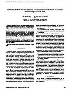
Separation process of a methane/butane mixture by the use of a ... Pressure Outlet (Permeate). Semi-permeable membrane x. C4H10. â 0.05 ... of Butane [g/h].
Predicting Performance and Efficiency of Semi‐Permeable Membranes with Simulation Thomas Eppinger1, Verena Kramer2, Nico Jurtz1, David Lucht2, Ravindra H. Aglave3, Matthias Kraume2 1
CD‐adapco, Nuremberg, Germany 2 Chair of Chemical and Process Engineering, Technische Universität Berlin, Berlin, Germany 3 CD‐adapco, Melville, NY
Outline 1. Motivation 2. Gas Separation Membrane 1. 2. 3. 4.
Numerical Set‐Up Modeling of membrane diffusion process Validation Results
3. Reverse Osmosis Desalination Membrane 1. 2. 3. 4.
Numerical Set‐Up Modeling of membrane diffusion process Validation Results
4. Conclusion
Motivation / Application • Membrane processes are widely used in the industry • Lower investments compared to other classical methods • Computational Fluid Dynamics (CFD) may help to optimize the design Example 1: Separation process of a methane/butane mixture by the use of a mixed‐matrix membrane Example 2: Desalination process by the use of a reverse osmosis membrane
Simulation of a gas separation membrane using STAR‐CCM+
Geometry and Boundary Conditions Pressure Outlet (Retentate) Velocity Inlet (Feed): xC4H10 0.05 xCH4 0.95
Semi-permeable membrane Pressure Outlet (Permeate)
Meshing • Trimmed Mesh • 280 000 Volume Cells • Prism Layer : • Thickness: 0.2mm • 3 Prism layers • Prism Layer Refinement at Membrane: • Thickness: 0.3mm • 10 Prism layers at the membrane surface to capture the concentration layer
Models used • • • • •
Multi‐component gas Multi‐component diffusion vs. Sc=1 Real Gas (Redlich‐Kwong) Coupled Solver k‐‐SST Turbulence Model Diffusion process through membrane is implemented via an interpolate table field function approach.
Modelling the membrane diffusion process Li – Permeance of species i [kg/(m^2 s Pa)] fi – Fugacity of species i [Pa] P – Absolute Pressure [Pa] xi – Mole fraction of species i [‐] i – Fugacity coefficient of species i [‐]
· Δf ·
·
Calculation of fugacity coefficient1: 2·
·
2·
·
2 2
1
1Bal
1
1
2 3
K. Kaul, John M. Prausnitz,1977, Second Virial Coecients of Gas Mixtures Containing Simple Fluids and Heavy Hydrocarbons. Industrial and engineering chemistry, Fundam., Vol 16, No. 3 pp. 335-340
Mole Fraction Butane @ Permeate Outlet [‐]
Validation against experimental results 0.35
0.30
0.25
0.20
0.15
0.10
0.05
0.00
10bar Experimental
20bar CFD (Sc=1)
30bar CFD (Chapman‐Enskog)
40bar
Results: Species Flow through Membrane 80
Species Flow of Butane [g/h]
70 60 50 40 30 20 10 0
10bar
20bar Sc=1
30bar Chapman‐Enskog
40bar
Results: Species Flux (Chapman‐Enskog) 6.0 5.5
Area of Membrane [%]
5.0 4.5 4.0 3.5 3.0 2.5 2.0 1.5 1.0 0.5 0.0 0.0005
0.0010
0.0015
0.0020
0.0025
0.0030
0.0035
0.0040
0.0045
0.0050
Species Flux of Butane through Membrane [kg/m2s] 40bar
30bar
20bar
10bar
0.0055
0.0060
Results: Flow Field (10bar)
Results: Concentration of Butane
10 bar
20 bar
30 bar
40 bar
Simulation of desalination in a membrane reverse osmosis reactor using STAR‐CCM+
Modelling the membrane diffusion process
Δ
· ∆ ·
∆
·
Ki – Permeation coefficient [m/(s Pa)] i – Osmotic pressure of species i [Pa] P – Absolute Pressure [Pa] xi – Mole fraction of species i [‐] T – Temperature [K] ‐ Specific Volume [m3/mol] ρi – Density [kg/m3] R – Universal Gas Constant [J/mol K]
Velocity Inlet:
Pressure Outlet
u0=0.2m/s cNaCl=2g/l
Feed Side
Permeate Side Membrane
Baffle
Meshing and Models used • • • • • • •
Steady Simulation Multi‐component fluid Density = f(xNaCl) Viscosity = f(xNaCl) Diffusion Coefficient = f(xNaCl) Coupled Solver Laminar Flow
Structured Mesh 544 000 cells
Diffusion process through membrane is implemented via an interpolate table field function approach.
Validation against experimental results2,3 33.6
35
Species Flux H2O [l/m2hr]
31.4 30
29.4 27.4
32.8
30.6
28.5
26.0
25 20 15 10 5 0 898.7kPa
998.7kPa
1098.7kPa
ΔP CFD 2A.
Experimental Data
Alexiadis, D.E. Wiley, A. Vishnoi, R.H.K. Lee, D.F. Fletcher, J. Bao. CFD modelling of reverse osmosis membrane flow and validation with experimental results. Desalination 217. 242-250. (2007) 3D.F. Fletcher, D.E. Wiley. A computational fluid dynamics study of buoyancy effects in reverse osmosis. Journal of Membrane Science 245. 175-181. (2004)
1198.7kPa
Results: Concentration of NaCl on membrane surface
Increasing Pressure
Conclusion • Successfully validated the approach • Showed an efficient way to simulate membrane processes • The approach is universal: Almost any flux model can be implemented • Deeper insight into the system • An efficient tool to improve the design
Thanks for your attention!