Predicting Protein Secondary Structure Using ... - Springer Link

Machine Learning, 29, 275–301 (1997)

c 1997 Kluwer Academic Publishers. Manufactured in The Netherlands. °

Predicting Protein Secondary Structure Using Stochastic Tree Grammars* NAOKI ABE HIROSHI MAMITSUKA

[email protected] [email protected]

Theory NEC Laboratory, Real World Computing Partnership C & C Media Research Laboratories, NEC Corporation, 4-1-1 Miyazaki, Miyamae-ku, Kawasaki, 216 Japan. Editor: Pat Langley Abstract. We propose a new method for predicting protein secondary structure of a given amino acid sequence, based on a training algorithm for the probability parameters of a stochastic tree grammar. In particular, we concentrate on the problem of predicting β-sheet regions, which has previously been considered difficult because of the unbounded dependencies exhibited by sequences corresponding to β-sheets. To cope with this difficulty, we use a new family of stochastic tree grammars, which we call Stochastic Ranked Node Rewriting Grammars, which are powerful enough to capture the type of dependencies exhibited by the sequences of β-sheet regions, such as the ‘parallel’ and ‘anti-parallel’ dependencies and their combinations. The training algorithm we use is an extension of the ‘inside-outside’ algorithm for stochastic context-free grammars, but with a number of significant modifications. We applied our method on real data obtained from the HSSP database (Homology-derived Secondary Structure of Proteins Ver 1.0) and the results were encouraging: Our method was able to predict roughly 75 percent of the β-strands correctly in a systematic evaluation experiment, in which the test sequences not only have less than 25 percent identity to the training sequences, but are totally unrelated to them. This figure compares favorably to the predictive accuracy of the state-of-the-art prediction methods in the field, even though our experiment was on a restricted type of β-sheet structures and the test was done on a relatively small data size. We also stress that our method can predict the structure as well as the location of β-sheet regions, which was not possible by conventional methods for secondary structure prediction. Extended abstracts of parts of the work presented in this paper have appeared in (Abe & Mamitsuka, 1994) and (Mamitsuka & Abe, 1994). Keywords: Stochastic tree grammars, protein secondary structure prediction, beta-sheets, maximum likelihood estimation, minimum description length principle, unsupervised learning.

1.

Introduction

Protein is made of a sequence of amino acids that is folded into a three-dimensional structure. Protein secondary structures are relatively small groups of protein structures exhibiting certain notable and regular characteristics, that function as intermediate building blocks of the overall three-dimensional structure and can be classified into three types; α-helix, βsheet, and others. In the present paper, we propose a new method for predicting the protein secondary structure of a given amino acid sequence, based on a classification rule automatically learned from a relatively small database of sequences whose secondary structures have been experimentally determined. Among the above three types, we concentrate on the problem of predicting the β-sheet regions in a given amino acid sequence. Our method receives as input amino acid sequences known to correspond to β-sheet regions, and trains *

Both authors contributed equally to this work.

276

N. ABE AND H. MAMITSUKA

the probability parameters of a certain type of stochastic tree grammar so that its distribution best approximates the patterns of the input sample. Some of the rules in the grammar are intended a priori for generating β-sheet regions and others for non-β-sheets. After training, the method is given a sequence of amino acids with unknown secondary structure, and uses the learned rules to predict regions that correspond to β-sheet rules, based on the most likely parse for the input sequence. The problem of predicting protein structures from their amino acid sequences is probably the single most important problem in genetic information processing, with immense scientific significance and broad engineering applications. Recently, increasing attention has been given to the methods for three-dimensional structural prediction that attempt to predict the entire protein structure, such as ‘homology modeling’ (c.f., May & Blundell, 1994) and ‘inverse folding’ (c.f. Wodak & Rooman, 1993). These methods are based on alignment/scoring of the test sequence against sequences with known structure, and therefore are not effective for those sequences having less than 25 percent sequence similarity to the training sequences (Sander & Schneider, 1991). At the other end of the spectrum is protein secondary structure prediction, which is general in the sense that it does not rely on alignment with sequences having known structure and hence can be applied on sequences having little or no sequence similarity, but it also provides less information. The present paper aims at providing a general method that can be applied to sequences with less than 25 percent sequence similarity, and yet provides more structural information. The classical problem of secondary structure prediction involves determining which regions in a given amino acid sequence correspond to each of the above three categories (Qian & Sejnowski, 1988; Rost & Sander, 1993; Cost & Salzberg, 1993; Barton, 1995). There have been several approaches for the prediction of α-helix regions using machine learning techniques that have achieved moderate success. Prediction rates between 70 to 80 percent, varying depending on the exact conditions of experimentation, have been achieved by some of these methods (Mamitsuka & Yamanishi, 1995; Muggleton, King, & Sternberg, 1992; Kneller, Cohen, & Langridge, 1990). The problem of predicting β-sheet regions, however, has not been treated at a comparable level. This asymmetry can be attributed to the fact that β-sheet structures typically range over several discontinuous sections in an amino acid sequence, whereas the structures of α-helices are continuous and their dependency patterns are more regular. To cope with this difficulty, we use a certain family of stochastic tree grammars whose expressive powers exceed not only that of hidden Markov models, but also stochastic contextfree grammars (SCFGs).1 Context-free grammars are not powerful enough to capture the kind of long-distance dependencies exhibited by the amino acid sequences of β-sheet regions. This is because the β-sheet regions exhibit ‘anti-parallel’ dependency (of the type ‘abccba’), ‘parallel’ dependency (of the type ‘abcabc’), and, moreover, various combinations of them (e.g., as in ‘abccbaabcabc’). The class of stochastic tree grammars that we employ in this paper, the Stochastic Ranked Node Rewriting Grammar (SRNRG), is one of the rare families of grammatical systems that have both enough expressive power to cope with all of these dependencies and at the same time enjoy relatively efficient parsability and learnability.2

PREDICTING PROTEIN SECONDARY STRUCTURE

277

The Ranked Node Rewriting Grammars (RNRG) were briefly introduced in the context of computationally efficient learnability of grammars by Abe (1988), but its formal properties as well as basic methods such as parsing and learning algorithms were left for future research. The discovery of RNRG was inspired by the pioneering work of Joshi, Levy, and Takahashi (1975) and of Vijay-Shanker and Joshi (1985) on a tree grammatical system for natural language called ‘Tree Adjoining Grammars’, but RNRG generalizes tree adjoining grammars just in a way that is suited to capture the type of dependencies present in the sequences in β-sheet regions. For example, tree adjoining grammars can handle a single parallel dependency, which cannot be handled by context-free grammars, but cannot deal with a complicated combination of anti-parallel and parallel dependencies. All of such dependencies can be captured by some members of the RNRG family. The learning algorithm we use is an extension of the ‘inside-outside’ algorithm for the stochastic context-free grammars (Jelinik, Lafferty, & Mercer, 1990), and is also related to the extension of the inside-outside algorithm developed for the stochastic tree adjoining grammars by Schabes (1992). These are all iterative algorithms guaranteed to find a local optimum for the maximum likelihood settings of the rule application probabilities. We emphasize here that our algorithm learns the probability parameters of a given grammar, and not the structure of that grammar.3 Perhaps the most serious difficulty with our method is the amount of computation required by the parsing and learning algorithms.4 The computational requirement of the learning algorithm is brought down drastically by using the so-called ‘bracketing’ technique. That is, when training an SRNRG fragment corresponding to a certain β-sheet region, rather than feeding the entire input sequence to the learning algorithm, it receives the concatenation of just those substrings of the input sequence that correspond to the β-sheet region. In contrast, the parsing algorithm must process the entire input string, as it clearly does not know in advance which substrings in the input sequence correspond to the β-sheet region. Hence most of the computational requirements are concentrated in the parsing algorithm. In order to reduce the computational expense of parsing, we have restricted the form of grammars to a certain subclass of RNRG that we call ‘linear RNRG,’ and we have devised a simpler and faster algorithm for this subclass. This subclass is obtained by placing the restriction that the right-hand side of any rewrite rule contains at most one occurrence of a non-terminal, excepting lexical non-terminals. This significantly simplifies the parsing and learning algorithms, as the computation of each entry in the parsing table becomes much simpler. In addition, we parallelized our parsing algorithm and implemented it on a 32-processor CM-5 parallel machine. We were able to obtain a nearly linear speed-up, which let the system predict the structure of a test sequence of length 70 in about nine minutes, whereas the same task took our sequential algorithm almost five hours. We also employed a method of reducing the alphabet size5 (i.e., the number of amino acids) by clustering them (at each residue position), using MDL (minimum description length) approximation (Rissanen, 1986) and their physico-chemical properties, gradually through the iterations of the learning algorithm.6 That is, after each iteration of the learning algorithm, the system attempts to merge a small number of amino acids, if doing so reduces the total description length (using the likelihood calculation performed up to that point).

278


We tested our method on real data obtained from the HSSP (Homology-derived Secondary Structure of Proteins Ver 1.0, Sander & Schneider, 1991) database of the European Molecular Biology Laboratory.7 The results indicate that the method can capture and generalize the type of long-distance dependencies that characterize β-sheets. Using an SRNRG trained by data for a particular protein (consisting of a number of sequences aligned to that protein sequence in HSSP), the method was able to predict the location and structure of β-sheets in test sequences from a number of different proteins, which have similar structures but have less than 25 percent pairwise sequence similarity to the training sequences. Such a prediction problem belongs to what is sometimes referred to in the literature as the ‘Twilight Zone’ (Doolittle et al., 1986), where alignment is no longer effective. Furthermore, we conducted a systematic evaluation experiment in which proteins used for training and those for testing had almost no sequence similarity and their structures had no apparent relationship. Our method was able to identify roughly 75 percent of the β strands as such, 80 percent of which were predicted correctly including their orientation with respect to the sterically neighboring strand. With respect to the more usual measure of residue-wise prediction accuracy of the binary classification problem (distinguishing between β-sheet regions from non-β-sheet regions), our method achieved about 74 percent. This figure is comparable to the state-of-the-art prediction methods in the literature, although our experiment involved only a certain restricted type of β-sheet structures and the testing was done on relatively small amounts of data. We emphasize that, unlike previous methods for secondary structure prediction, our approach can predict the structure of the β-sheet, namely the locations of the hydrogen bonds. 2. 2.1.

Stochastic tree grammars and β-sheet structures Stochastic ranked node rewriting grammars

We will first informally describe the Ranked Node Rewriting Grammar (RNRG) formalism and then give its definition in full detail. An RNRG is a tree-generating system that consists of a single tree structure called the starting tree and a finite collection of rules that rewrite a node in a tree with an incomplete tree structure. The node to be rewritten must be labeled with a non-terminal symbol, whereas the tree structure can be labeled with both non-terminal and terminal symbols. Here we require that the node being rewritten has the same number of child nodes (called the ‘rank’ of the node) as the number of ‘empty nodes’ in the incomplete tree structure. After rewriting, the children of the node are attached to these empty nodes in the same order as before rewriting. The tree language generated by an RNRG grammar is the set of all trees whose nodes are labeled solely with terminal symbols that can be generated from the starting tree by a finite number of applications of its rewrite rules. The string language of the grammar is the set of yields from the trees in its tree language, namely the strings that appear on the leaves of the trees, read from left to right. We will now give detailed definitions. (i) The set of labeled directed trees over an alphabet Σ is denoted TΣ . (ii) The rank of an “incomplete” tree is the number of empty nodes in it. (iii) The rank of a node is the number of direct descendants. (iv) The rank of a symbol is defined if the rank of any node labeled by it is always the same and equals that rank. (v) A


279

ranked alphabet is one in which every symbol has a rank. (vi) We write rank(x) for the rank of x, be it a node or a symbol. Definition. A ranked node rewriting grammar G is a quintuple hΣN , ΣT , ], βG , RG i, where: (i) ΣN is a ranked nonterminal alphabet. (ii) ΣT is a terminal alphabet disjoint from ΣN . We let Σ = ΣN ∪ ΣT . (iii) ‘]’ is a distinguished symbol distinct from any member of Σ, indicating “an empty node.” 8 (iv) βG is a labeled tree over Σ. We say that βG is the ‘starting tree’ of the grammar. (v) RG is a finite set of rewrite rules: RG ⊂ {hA, αi | A ∈ ΣN & α ∈ TΣ∪{]} & rank(A) = rank(α)}. Henceforth, we write A → α for rewrite rule hA, αi. (vi) rank(G) = max {rank(A) | A ∈ ΣN }. We emphasize that the distinction between nonterminal symbols and terminal symbols described above does not coincide with that between internal nodes and frontier nodes of derived trees. (See the example derivation given in Figure 4.) Definition. We say ‘G derives α from β in one step’ if there is hA, γi ∈ RG such that some node η of α is labeled by A, and β is the tree obtained by replacing η in α by γ, with the children of η attached to the empty nodes in γ preserving their relative order. We write α `G β and let `∗G denote the transitive closure of the `G relation. The tree language of a grammar is defined as the set of trees over the terminal alphabet that can be derived from the grammar. This is analogous to the way the string language of a rewriting grammar is defined in the Chomsky hierarchy. Definition. The tree language and string language of an RNRG G, denoted T(G) and L(G), respectively, are defined as: T (G) = {β ∈ TΣT | βG `∗G β} L(G) = {yield(β) | β ∈ T (G)}. If we now place an upper bound, say k, on the rank of a node that can be rewritten, we obtain a family of grammars, RNRG(k), each of which has varying expressive power. Definition. For each k ∈ N we let RNRG(k) = {G ∈ RNRG | rank(G) ≤ k }. For each k ∈ N we let RNRL(k) = {L(G)|G ∈ RNRG(k)}. In the ‘RNRG hierarchy’ defined above, one can easily verify that RNRL(0) equals the class of context-free languages, and RNRL(1) equals the class of tree adjoining languages. Furthermore, for any k ≥ 2, RNRL(k) properly contains RNRL(k − 1). For example, for each k, RNRL(k) contains the 2(k + 1) count language, namely the language {an1 an2 ...an2(k+1) |n ∈ N }, but RNRL(k − 1) does not. We now give some examples of

280


Starting Tree

Rewrite Rules (α 3) S

S

(β)

λ (α 1)

t # t

t a

S

a

S

(α 2)

b

S

t a

S

b

t a

#

b

#

b

Figure 1. RNRG(1) grammar G1 generating {wwR wwR |w ∈ {a, b}}.

t (β) S

t (α1) a

λ a

S t λ

a

(α2 )

a b

t S

t a b

(α3)

a

t

a

b

t

b

t

t

a b a

t λ

b

b

a

a

t λ

b a

Figure 2. Derivation of ‘abbaabba’ by an RNRG(1) grammar.

RNRG grammars. The language L1 = {wwR wwR |w ∈ {a, b}∗ } is generated by the RNRG(1) grammar G1 shown in Figure 1, where wR denotes the string obtained by ‘reversing’ w. 9 Figure 2 illustrates the way the derivation in RNRG takes place for the string ‘abbaabba’ by grammar G1 . We note that L1 can be generated by a tree adjoining grammar, but the ‘three copy’ language, L2 = {www | w ∈ {a, b}∗ } cannot (c.f., Vijay-Shanker & Joshi, 1985). This language can be generated by the RNRG(2) grammar G2 shown in Figure 3. Figure 4 traces the derivation of the string ‘ababab’ by G2 . Each of the trees shown in Figure 4 is called a ‘partially derived tree.’ As the figure indicates, the tree structure introduced by a particular rule may be split into several pieces in the final derived tree, unlike usual parse trees in a context-free grammar. (The parts of the derivation tree generated by rule α1 are drawn with darker lines.) It is easy to see that the three occurrences of letter ‘a’

281


are generated by a single application of rule α1 and its ‘cross-serial’ dependency therefore is captured by a single rule.

Starting Tree

Rewrite Rules (α3 ) S

S

(β) λ

t

λ

#

#

t a

(α1 ) S

t λ

S

t λ

(α2 ) S

b

t aλ #

#

λ

S

t λ

a

#

t bλ #

b

Figure 3. RNRG(2) grammar G2 generating {www|w ∈ {a, b}∗ }.

t

(α 1)

S

a S

λ

a

t

(β)

λ

t λ

λ

t λ

(α 2)

λ λ

b

λ

t

t

(α 3) b

t

a λ

t

b λ

t

λ

λ

a λ

λ

λ

a

S t

a λ

t

t

t

λ t

b

λ

t

b λ

t

b

a

λ

λ

a λ

λ

a

Figure 4. Derivation of ‘ababab’ by an RNRG(2) grammar.

Given the definition of RNRG, the stochastic RNRG is defined analogously to the way a stochastic context-free grammar is defined from a context-free grammar. That is, associated with each rewrite rule in a stochastic RNRG is its rule application probability, which is constrained so that, for each non-terminal, the sum of the application probabilities of all the rewrite rules for that non-terminal equals unity. This way, each stochastic RNRG can be viewed as a probabilistic generator of finite strings, and thus defines a probability distribution over the set of all finite strings.10 For example, if we assign the probabilities 0.5, 0.3, and 0.2 to the three rewrite rules α1 , α2 , and α3 in G2 , then it generates the string ‘ababab’ with probability 0.5 · 0.3 · 0.2 = 0.03.

282 2.2.


Modeling β-sheet structures with RNRG

As we noted in the introduction, the prediction of the β-sheet regions has been considered difficult because of the long-distance dependencies exhibited by the corresponding regions. This is illustrated by the schematic representation of typical β-sheet structures given in Figure 5.

(a)

(c)

(b)

(d)

Figure 5. Some typical β-sheet structures.

The arrows indicate the β-sheet strands and the line going through them represents the amino acid sequence. The β-sheet structure is retained by hydrogen bonds (H bonds) between the corresponding amino acids in neighboring strands, so it is reasonable to suspect that there are correlations between the amino acids in those positions. The structure exhibited in Figure 5 (a) is known as an ‘anti-parallel’ β-sheet, as the dependency follows the pattern abc . . . cba . . . abc . . . cba, where use of the same letter indicates that those positions are connected by H bonds11 and believed to be correlated. In contrast, the structure exhibited in Figure 5 (b) is known as a ‘parallel’ β-sheet, since the dependency here is more of the pattern of abc . . . abc . . .. Both types of dependency can be captured by RNRG, in particular, G1 in Figure 1 and G2 in Figure 3, respectively. (See also Figure 2 and Figure 4.) There are β-sheet structures that contain both of these types of dependency, such as that shown in Figure 5 (c). Note that the structure of this figure is the same as the β-sheet pattern for one of the proteins used in our experiments, which appears in Figure 6.12 These β-sheet structures can be handled by a grammar like G1 , except each of the trees on the right-hand sides of the rules (α1 ) and (α2 ) have one of the terminal symbols (the one on the right lower corner) missing. These structures can be combined to obtain larger β-sheets, as is shown in Figure 5 (d), and can result in a high degree of complexity. If we use an RNRG of a higher rank, however, such dependencies can be handled. For example, the dependency pattern of Figure 5 (d) can be expressed by the RNRG(3) grammar given in Figure 7.

283


Figure 6. Three-dimensional view of an actual β-sheet structure.

Rewrite Rules

Starting Tree S

(β) λ

(α 3)

λ

t S

λ

# t

(α 1)

a S t a # a a

S t

#

#

t a

b

(α ) S 2 t

# a a # a

S

t

t

b #

b b #

b t b b # b

Figure 7. An RNRG(3) grammar generating {wwR wwR wwR wwR |w ∈ {a, b}∗ }.

Note also that there can be insertions of irrelevant (i.e., non-β-sheet) regions between the sub-regions, resulting in a sequence like abcxyyzxabczzxz, where x, y, z are irrelevant letters. The irrelevant letters x can be introduced by simple rank 1 rewrite rules of the form S → t(x, S(])) and S → t(S(]), x), where ] denotes an empty node.

284 3.


Learning and parsing of a restricted subclass

The ‘linear’ subclass of SRNRG we use in this paper is the subclass satisfying the following three constraints: (i) The right-hand side of each rewrite rule contains at most one node labeled with a non-terminal symbol of rank greater than zero; (ii) Every other non-terminal (of rank 0) is a specially designated ‘lexical’ non-terminal, say A, such that all rewrite rules for A are lexical rules, namely rules of the form A → a for some a ∈ ΣT ; (iii) Each ‘consecutive’ portion of the right-hand side of every rewrite rule contains at most one lexical non-terminal. For rank 1 SRNRG, in particular, this means that there is at most one lexical non-terminal in each of the four corners (left up, left down, right up and right down) of the unique (if any) non-terminal on the right-hand side. Examples of SRNRG of rank 1 satisfying these constraints can be found in Figure 10(a). Note that each occurrence of a lexical non-terminal can be thought of as defining a distribution over the alphabet, and this is written in as part of the rule in the figure. In our current scenario, in which the terminal alphabet equals the amino acids, the rule application probabilities for these lexical rules are called ‘amino acid generation probabilities.’ Some structural prediction methods based on stochastic context-free grammars view the amino acid generation probabilities of all lexical non-terminals in a given rule as part of a joint probability distribution, making it possible to capture the correlations that may exist between them (Sakakibara et al., 1994; Eddy & Durbin, 1994). Although we treat the distribution at each non-terminal as being independent, a comparable effect can be achieved by training multiple copies of the same rule, as we report in subsection 4.2. With the above three constraints, the parsing and learning algorithms can be significantly simplified. For general SRNRG, the entries in the table used in the extended inside-outside algorithm (indexed by a 2(k + 1)-dimensional array) must be node-addresses of the tree structures appearing in the rewrite rules of the grammar, paired with their probabilities of generating the designated sections of the input string. With constraint (i), it suffices to place just the non-terminals (and the rewrite rules in the case of parsing) in the table entries, paired with their probabilities. These constraints also imply that the ‘yield’ of any particular rule consists of at most 2(k + 1) sections in the input string, and hence can be found in ‘one shot.’ Note that, in a general SRNRG, there is no a priori limit on how many pieces the yield of any given rule body can be divided into (though it is bounded above by a constant depending on the grammar) and thus they cannot be found in ‘one shot’ even if all the 2(k + 1) tuples of sub-strings of the input string are inspected. 3.1.

The learning algorithm

Our learning algorithm is an extension of the ‘inside-outside’ algorithm for stochastic context-free grammars, which is itself an extension of the Baum-Welch algorithm (or the ‘forward-backward’ algorithm) for the hidden Markov models. All of these algorithms are local optimization algorithms for the maximum likelihood settings of the rule application probabilities in the input model or grammar. We emphasize again that a fixed model/grammar is given as input – they are not learned from the data. For ease of exposition, we will first explain the basic ideas behind the Baum-Welch algorithm for hidden


285

Markov model (c.f., Levinson, Rabiner, & Sondhi, 1983) and then describe how it is extended for stochastic ranked node rewriting grammars. The Baum-Welch algorithm consists of the procedures for calculating the ‘forward’ probabilities and ‘backward’ probabilities, and for re-estimating the rule application probabilities and symbol generation probabilities in terms of these probabilities. The forward probability of a certain state i in an hidden Markov model at time step t is the probability that the model generates the first t symbols of the input sequence and arrives at state i. The backward probability of i0 at t0 is the probability that the model will generate the rest (all but the first t0 symbols) of the input sequence given that it is now at state i0 . Using these probabilities, one can calculate the sum (over arbitrary time step t) of the probabilities that the model is at state i at time t and goes to i0 at t + 1 and generates the entire input sequence, as well as the sum of the probabilities that the model is at state i at time t and generates the input sequence. The transition probability from state i to i0 is then re-estimated to be the ratio between the above two probabilities, calculated using the probability parameter values from the previous iteration. It is well-known (Levinson, Rabiner, & Sondhi, 1983) that this re-estimation is guaranteed to increase the likelihood given to the input sample, and hence iterative applications of this re-estimation results in a local optimum. For both stochastic context-free grammars and stochastic RNRG, the forward probability and the backward probability are generalized as ‘inside probability’ and ‘outside probability,’ which are no longer temporal notions. That is, forward/backward probability is defined for each position in the input string (which coincides with the time step), whereas inside/outside probability will be defined for a sequence of positions, as we will define shortly. Below, we will describe our training algorithm for the rank 1 stochastic RNRGs that adhere to the three constraints specified above. Let σ be the input amino acid sequence and let N be its length, and let σt denote the t-th letter (amino acid) of σ. Note that when we use the ‘bracketing’ technique, σ is a concatenation of the substrings corresponding to the β-sheet region of interest. We define the ‘inside probability’ of non-terminal S at i, j, k, l on σ, written Inσ [S, i, j, k, l], to be the sum of the probabilities of all partially derived trees whose root node is labeled by S and whose (two discontinuous) yields match the sub-strings from the i-th to j-th and from k-th to l-th letters of σ. Similarly, we define the ‘outside probability’ of non-terminal S at i, j, k, l, written Out[S, i, j, k, l], to be the sum of the probabilities of all partially derived trees whose (three discontinuous) yields match the sub-strings from the first to i-th, from j-th to k-th, and from l-th to N -th letters of σ, and contain S as the unique non-terminal. Now let G be the input grammar, and let N (G) denote the set of non-terminals of G. For each rewrite rule r in G, let T (r) denote the rule application probability of r, and L(r) and R(r) the non-terminal of the left-hand side and the (unique) non-terminal on the right-hand side of r, respectively. Let nrf , f = 1, ..., 4, denote the number (0 or 1) of terminal symbols at each of the four corners (left up, left down, right down, and right up) of the unique (if any) non-terminal symbol in the right-hand side of r, and Pfr (α), α ∈ A (|A| = 20) denote the generation probability of amino acid α at position f of r. Now we show how the inside and outside probabilities are calculated. The inside probabilities at arbitrary index (i, j, k, l) can be defined recursively solely in terms of the inside probabilities of its sub-intervals, so it can be calculated as long as one has already com-

286


puted the inside probabilities at those (i0 , j 0 , k 0 , l0 ) such that i ≤ i0 , j 0 ≤ j, k ≤ k 0 , l0 ≤ l. The looping used in the procedure for calculating inside probabilities exhibited in Table 1 ensures that this condition is satisfied. The outside probabilities can be calculated in a Table 1. Method for calculating the inside probabilities within the extended inside-outside algorithm. For i := N to 1 For j := i to N For k := N to j + 1 For l := k to N For S ∈ N (G)

X

Inσ [S, i, j, k, l] =

{ T (r) · Inσ [R(r), i+nr1 , j −nr2 , k+nr3 , l−nr4 ]·

{r∈G|L(r)=S} r r r r (P1r (σi+1 ))n1 (P2r (σj−1 ))n2 (P3r (σk+1 ))n3 (P4r (σl−1 ))n4

}

similar fashion, as shown in Table 2. Table 2. Method for calculating the outside probabilities within the extended inside-outside algorithm. For i := 1 to N For j := N to i + 1 For k := j to N For l := N to k + 1 For S ∈ N (G)

X

Outσ [S, i, j, k, l] =

{ T (r) · Outσ [L(r), i−nr1 , j +nr2 , k−nr3 , l+nr4 ]·

{r∈G|R(r)=S} r r r r (P1r (σi−1 ))n1 (P2r (σj+1 ))n2 (P3r (σk−1 ))n3 (P4r (σl+1 ))n4

}

Now if we let P rσ [r, i, j, k, l] denote the probability that the grammar generates the input sequence σ and uses rule r at the (i, j, k, l) position, then it can be calculated by the equality: P rσ [r, i, j, k, l] =Outσ [L(r), i, j, k, l] · Inσ [R(r), i+nr1+1, j −nr2−1, k+nr3 +1, l−nr4−1] r r r r ·T (r) · (P1r (σi+1 ))n1 (P2r (σj−1 ))n2 (P3r (σk+1 ))n3 (P4r (σl−1 ))n4 Let Uσ (r) denote the ‘weighted average frequency’ of rewrite rule r, namely the average frequency of r in a single parse of σ, weighted according to the generation probability of each parse using the current setting of the probability parameters. Similarly, define Vσr,f (α) to be the weighted average frequency of amino acid α at position f in rule r in a single parse of σ. More precisely, we define (we show the case f = 1 only for Vσr,f ): P P P P i j k l P rσ [r, i, j, k, l] Uσ (r) = P (σ) P P P P P Vσr,1 (α)

=

i

j

k

l

σi+1 =α

P (σ)

P rσ [r, i, j, k, l]

.


287

Finally, from Uσ (r) and Vσr,f (α), the update values for the rule application probabilities T (r) and the amino acid generation probabilities Pfr (α) can be calculated by the formulas P T (r) = P

P

σ∈Ξ

{r 0 ∈G|L(r 0 )=L(r)}

σ∈Ξ

P Pfr (α)

=P

Uσ (r)

σ∈Ξ

P

σ∈Ξ

Vσr,f (α) α0

Vσr,f (α0 )

Uσ (r0 )

,

where Ξ denotes the input sample. The above process is repeated until some stopping condition is satisfied, usually until the changes in the probability parameters become smaller than a certain preset amount. 3.2.

Reducing the alphabet size with MDL approximation

Since there are twenty amino acids and hence the alphabet size is twenty, it is difficult to estimate the amino acid generation probabilities at each position with reasonable accuracy with the small data size we have available in practice. Taking advantage of the fact that ‘similar’ amino acids tend to be easily substitutable, we cluster the amino acids at each residue position to effectively reduce the alphabet size. The obvious trade-off that we must resolve is between having a fine clustering, and thereby gaining high discriminability, and having a coarse clustering, and thereby achieving more accurate estimation. In order to resolve this trade-off, we make use of the MDL (minimum description length) principle (Rissanen, 1986), which gives a criterion for an optimal clustering relative to a given data size. We now describe our clustering method in some detail. After each iteration of the learning algorithm, the algorithm merges some of the amino acids at each lexical rule if the merge reduces the total description length (approximated using the probability parameters calculated up to that point). For this purpose it makes use of the Euclidean distance between the 20 amino acids in the (normalized) two-dimensional space defined by their molecular weight and hydrophobicity. At each iteration, it selects the two among the clusters from the previous iteration that are closest to each other in the above Euclidean space and merges them to obtain a single new cluster, but only if the merge reduces the following approximation of ‘description length’: −m

X c∈C

P (c) log

P (c) |C| log m + . |c| 2

In the above, we let c ∈ C be the clusters, P (c) the sum of the generation probabilities for amino acids in the cluster c, and m the effective sample size, namely the weighted P frequency of the lexical rule in question in the parses of the input sample, i.e. m = σ∈Ξ Uσ (r). Note that the above approximation of ‘data description length’ by the average minus loglikelihood using the current values of the probability parameters is accurate only if those

288


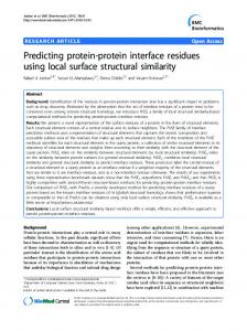
probability values are reliable. The algorithm keeps merging clusters in this fashion, but once it fails to merge one pair, it will not try to merge any other pair in the same iteration, in order to ensure that the merge process does not take place too fast at an early stage when the parameter estimation is particularly unreliable. Figure 8(a) illustrates the distribution of the 20 amino acids in the two-dimensional space defined by their molecular weights and hydrophobicity, based on the hydrophobicity measure given by Fauchere and Pilska (1983). We chose these two dimensions because the formation of β-sheet is considered to depend on the relative compatibility of corresponding amino acids (i.e., facing one another within a strand), in terms of ‘size’ (molecular weight) and ‘hydrophobicity.’13 Figure 8(b) shows an example of a clustering over them obtained by our method at some residue position in one of our experiments. The clustering obtained here is largely consistent with known classifications in the biochemistry literature (e.g., Taylor, 1986). Thus, our method gives a flexible clustering that is tailored to the conditions of each residue position, and that is also biologically meaningful. (b)

W Y

R K EQ DN

H

F M

T P S

L I V

C A G

Hydrophobicity

Molecular Weight

Molecular Weight

(a)

W Y

R K EQ DN

H T P S

F M L I V

C A G

Hydrophobicity

Figure 8. (a) Distribution of 20 amino acids in the two-dimensional space, and (b) an example of a clustering obtained by our method.

3.3.

Parallel parsing and prediction

For predicting the β-sheet regions of a test amino acid sequence whose secondary structure is unknown, we use the stochastic tree grammar that has been trained by the learning algorithm on a training data, and use it to parse the input sequence. We predict the regions generated by the ‘β-sheet rules’ in the grammar in the most likely parse of the inputP string to be β-sheet regions. The parsing algorithm can be easily obtained by replacing ‘ ’ by ‘max’ in the definition of the ‘inside’ algorithm, and retaining the most likely sub-parse at any intermediate step. As we noted in the introduction, we parallelized our parsing algorithm to run on a 32processor CM-5. In parallelizing this algorithm, we isolated the data dependency by in-

289


troducing into the outmost loop a parameter d, which stands for the total length of all the sub-strings that are inside those designated by the current indices. (d = (j − i) + (l − k) in the rank 1 case.) That is, we replace the first four For loops in the algorithm for calculating the outside probabilities by the four loops shown in Table 3. This way, the computation Table 3. For loops for parsing in parallel. For d := N to 1 For i := 0 to N − d For j := i + 1 to i + d For l := i + d to N

of all table entries for a given d can be performed in parallel. In particular, we allocate to each processor the computation for a block of consecutive values of i, each of size dN/32e or bN/32c, and let each of the processors request and receive necessary data from other processors by message passing. Note that constraint (iii) of the linear subclass ensures that for the computation of each entry (indexed by i, j, k, l) only those entries indexed by either i or i ± 1 are needed. Hence, message passing is required only when i is at an end of the consecutive block, and only between neighboring processors, resulting in a large savings in the amount of communication necessary between the processors. We now examine the speed-up obtained by our parallel parsing algorithm on the CM-5 in our experiments. Figure 9(a) shows the processing time (for parsing) in seconds, for input sequences of varying lengths, by our sequential parsing algorithm and by its parallel implementation on CM-5. Figure 9(b) shows the speed-up factor achieved by the parallel parsing algorithm as a function of the input length. For example, for input length of 70, our parallel implementation ran 31.4 faster than the sequential version, a nearly linear speed-up with 32 parallel processors.14 (a)

(b) 18000

35 parallel sequential

30

14000 speed-up factor

computation time

16000 12000 10000 8000 6000

25 20 15 10

4000 5

2000 0

20

30

40 50 60 sequence length

70

0

20

Figure 9. (a) The processing time (in seconds) and (b) the speed-up factor.

30

40 50 60 sequence length

70

290 4. 4.1.


Experimental results Cross-prediction with structurally similar proteins

We applied our method to real data obtained from the HSSP (Homology-derived Secondary Structure of Proteins Ver 1.0) database (Sander & Schneider, 1991). In all of our experiments, we used sequences listed in the PDB SELECT 25% list (Hoboem et al., 1992) for both training and test data. The PDB SELECT 25% list is a database containing sequences of protein with known structure possessing at most 25 % sequence similarity with one another, and thus it ensured that no test sequence had more than 25 % sequence similarity with any training data. For each of these sequences, we formed a ‘training data group’ by collecting the set of aligned sequences as having between 30 and 70 percent sequence similarity, according to the HSSP database. In what follows, we sometimes say we use a particular protein sequence as training data when we mean that we use all the sequences in its training data group. In our first experiment, we picked three different proteins, ‘Fasciculin’ (or ‘1fas’ in the code used in PDB SELECT 25%), ‘Caldiotoxin’ (1cdta) and ‘Neurotoxin B’ (1nxb), all of which are toxins. Although these three proteins have relatively similar structures (their common structure was shown in Figure 6), their sequences have less than 25 percent sequence similarity to one another, and hence alignment alone cannot detect this similarity. We trained a stochastic RNRG with training data consisting of bracketed sequences for one of the three proteins, say 1fas, and used the acquired grammar to predict the location of βsheet regions in an amino acid sequence of another one of the three, either 1cdta or 1nxb. By bracketing the input sequences, we mean that we isolated the (discontinuous) sub-strings of the training sequences that correspond to β-sheets from the rest, and trained the probability parameters of the ‘β-sheet rules’ in the grammar with them.15 The probability parameters of the non-β-rules were set to be uniform. We then used the acquired stochastic RNRG grammar to parse an amino acid sequence of either 1cdta or 1nxb, and predicted the location of β-sheet regions according to where the β-sheet rules are in the most likely parse. The system predicted the location of all three β-strands contained in the test sequence almost exactly (missing only one or two residues that were absent in all of the training data) in both cases. We carried out the analogous runs for all (six) possible combinations of the training data group and the test sequence from the three proteins. Our method was able to predict all three of the β-strands in all cases, except in predicting the location of β-sheet in the test sequence for 1cdta based on the training data group of 1nxb: The system failed to identify one of the three β-strands correctly in this case. Figure 10(a) shows the part of the stochastic RNRG(1) grammar obtained by our learning algorithm on the training set for 1fas that generates the β-sheet regions. Note that, in the figure, the amino acid generation probabilities at each position are written in a box. For example, the distribution at the right upper corner in (α4 ) gives probability 0.80 to the cluster {I, L, V } and probability 0.10 to the single amino acid Y . The interpretation of the grammar is summarized schematically in Figure 10(b). It is easy to see that the grammar represents a class of β-sheets of type (c) in Figure 5. Each of the rules (α1 ), (α2 ), (α3 ), (α4 ), (α6 ) and (α7 ) generates part of the β-sheet region corresponding to a row of amino


291

Figure 10. (a) A part of the acquired RNRG grammar and (b) its interpretation.

acids connected by H bonds and (α5 ) inserts an ‘extra’ amino acid that does not take part in any H bond. Rule (α4 ) says that in the third (from the top) row, amino acids I, L and V are equally likely to occur in the leftmost strand, and it is very likely to be K in the middle strand. Note that I, L, and V have similar physico-chemical properties, and it is reasonable that they were merged to form a cluster. Figure 11(a) shows the most likely parse (derived tree) obtained by the grammar on a test sequence of 1cdta. The shaded areas indicate the actual β-sheet regions, which are all correctly predicted. The seven types of thick lines correspond to the parts of the derived tree generated by the seven rules shown in Figure 10(a). The structural interpretation of this parse is indicated schematically in Figure 11(b), which is also exactly correct. Note that the distributions of amino acids in the acquired grammar are quite well spread over many amino acids. For example, none of the amino acids in the third strand of the test sequence, except the last two Cs, receives a dominantly high probability. The clustering of amino acids, therefore, was crucial for the grammar to predict the third strand of the β-sheet in the test sequence. 4.2.

Capturing correlations with multiple rules

One apparent shortcoming of the experiment we just described is that only one copy of each of the rules (α1 ), ..., (α7 ) was present in the trained grammar. As a result, each of the acquired rules could capture the distributions of amino acids at each residue position, but

292


Figure 11. (a) The parse of the test sequence and (b) its interpretation.

could not truly capture the correlations that exist between residue positions, even if they are captured by a single rule. We conducted another experiment using exactly the same data as in the above experiment, but that used multiple copies (two in particular) of each of the β-sheet rules (α1 ), ..., (α7 ). (Randomly generated numbers were used for the initial values of their probability parameters.) In the acquired grammar, some rules were split into a pair of rules that significantly differ from each other, while others became basically two copies of the same rule. An example of a rule that was split is (α3 ) in Figure 10(a); the two rules into which it split are shown in Figure 12(a). This split is meaningful because, in the new grammar, the joint distribution over the two nodes at the top are seen to be heavily concentrated on (K, {N, H}) and (N, {R, K}), which is finer than what we had in the previous grammar ({K, N }, {N, H, R, K}). This way, the grammar was able to capture the correlation between these residue positions, which are far from each other in the input sequence. We used the grammar containing two copies each of the β-sheet rules obtained using training data for 1fas to predict a test sequence for both 1cdta and 1nxb. As before, the locations of all three β-strands were predicted exactly correctly. Interestingly, distinct copies of some of the split rules were used in the respective most likely parses for 1cdta and 1nxb. For example, rule (α3 -1) was used in the most likely parse for the test sequence for 1cdta, and (α3 -2) for 1nxb. It seems to indicate that the training sequences for 1fas contained at least two dependency patterns for this bonding site, as shown in Figure 12(b): The corresponding bonding site in 1cdta was of the first type and the site in 1nxb was of the second type. The point just illustrated is worth emphasizing. If one tried to capture this type of correlation in bonding sites by a hidden Markov model, it would necessarily result in much higher complexity. For example, suppose that eight bonding sites in a row (say each with


293

Figure 12. (a) The two rules (α3 ) was split into and (b) their interpretations.

just two residue positions for simplicity) are split into two distinct rules. In a hidden Markov model, the eight rules would have to be realized by two copies each of consecutive states – sixteen states in a chain. Since there are 28 = 256 possible combinations of rules to use, the hidden Markov model would need 256 non-deterministic branches of state sequences, each corresponding to a possible combination of the eight options. In the case of stochastic tree grammar, we only needed 2 × 8 rules. Clearly this huge reduction in complexity is made possible by the richer expressive power of stochastic tree grammars.

4.3.

Systematic performance evaluation

The experiments described so far involved proteins that do not have notable sequence similarity but still share very similar structures. In this subsection, we will describe systematic experiments we conducted in which the sequences used for training and those for testing have no apparent relation at all. In particular, we selected all proteins containing a fourstrand β-sheet pattern of the type shown in Figure 5(a) in isolation (which we will call ‘type a’) satisfying a certain condition to ensure that they are all unrelated. For each of the selected proteins, we formed a ‘data group’ consisting of aligned sequences for that protein sequence. We then obtained a stochastic grammar fragment for each of the data groups, using the sequences in that data group as training data. We then attempted to predict the structure and location of the β-sheet region in test sequences that are similarly selected but unrelated to the training sequences, using the stochastic grammar fragments of all data groups. We describe the details of this experiment below.

294


Table 4. Training data used in the experiment.

4.3.1.

PDB code

protein

1aak 1apm E 1dlh B 1ppn

UBIQUITIN CONJUGATING ENZYME (E.C.6.3.2.19) $C-/AMP$-DEPENDENT PROTEIN KINASE (E.C.2.7.1.37) HLA-DR1 HUMAN CLASS II HISTOCOMPATIBILITY PAPAIN CYS-25 WITH BOUND ATOM

no. of alignments 19 107 20 56

The data

We again used the aligned data available in HSSP database. As training data, we used sequences containing four-strand patterns of type a such that their aligned sequences are reasonable as training data. More precisely, we used all (and therefore unbiased) sequences satisfying four conditions: 1. The ‘key sequence,’ to which the other sequences in the group are aligned, is that of a protein contained in the PDB SELECT25% list (Hoboem et al., 1992). This ensures that no two key sequences have 25% or more sequence homology. 2. It contains a four-strand β-sheet pattern of type a in isolation, not as part of a larger β-sheet pattern. 3. In at least 18 of the sequences aligned to the key sequence as having 30 % to 70 % sequence similarity in HSSP, β-strands corresponding to all four β-strands in the key sequence are present. 4. Each β-strand has length at least three. We obtained four proteins in this way (containing one four-strand pattern each) which we list in Table 4. We call the set of aligned data for each of the above proteins a ‘training data group.’ Thus, our training data consist of a number of groups of sequences that are similar and alignable within the groups, but that are dissimilar (< 25% homology) and non-alignable across the groups. The test data were similarly selected, except the additional condition on the aligned sequences was replaced by a length bound. More precisely, we extracted all (and therefore unbiased) sequences satisfying the four conditions: 1. It is contained in the PDB SELECT25% list. 2. It contains a 4-strand β-sheet pattern of type a in isolation, not as part of a larger β-sheet pattern. 3. Its length does not exceed 120. 4. It is not contained in the training data. We introduced the third condition for efficiency reasons. We obtained five test data in this way, which are shown in Table 5.


295

Table 5. Test data used in the experiment.

4.3.2.

PDB code

protein

1bet 1bsa A 1cska 1tfi 9rnt

BETA-NERVE GROWTH FACTOR BARNASE (G SPECIFIC ENDONUCLEASE) (E.C.3.1.27.-) MUTANT C-SRC KINASE (SH3 DOMAIN) (E.C.2.7.1.112) TRANSCRIPTIONAL ELONGATION FACTOR SII RIBONUCLEASE T=1= (E.C.3.1.27.3)

Training and prediction procedures

We manually constructed a tree grammar fragment (consisting only of β-sheet rules) for each of the four training data groups, and then trained the probability parameters in it, using as training data all the aligned sequences in that group. In doing so, we set the initial amino acid distribution at each leaf node to be uniform. As we stated earlier, we employed the bracketing technique, namely of extracting the β-strand portions in the training data and training the β-sheet rules of each grammar fragment with them. The prediction was done by analyzing the input sequence using each of the grammar fragments trained on the training data groups, and taking the location and structural pattern of the most likely analysis among them all, i.e., the analysis that was given the highest probability. Henceforth, we refer to this prediction method as ‘MAX.’ 4.3.3.

The results

The results of these prediction experiments are shown in Table 6 (under the columns for MAX). In the table, ‘#located’ denotes the number of strand positions predicted by MAX that have non-empty intersections with the actual β-strands of the test sequence, and ‘#paired’ denotes the number of strands among these, that are correctly paired with a sterically neighboring strand, including their relative orientation. The result on #located indicates that 75 percent (15 out of 20) of the strands that were predicted had a non-empty intersection with an actual strand. As for #paired, 80 percent of these locations (and 60 percent overall) had a correct local structure as well. For comparison we also tested the performance of a naive randomized prediction method. The randomized prediction method, which we call RAND, randomly picks four strand regions, each of length six (which is the average length of a β-strand in the training data) and predicts accordingly. The results for RAND are shown in Table 6, each averaged over ten trials. We observe that the total #paired for RAND is about three, and is significantly lower than that of MAX. We also calculated the more usual measure of residue-wise prediction accuracy of the binary classification problem (distinguishing between β-sheet regions and non-β-sheet regions). Table 7 gives the details of this analysis: Our method correctly predicted roughly 74 percent of the residues in the five test sequences. This figure compares well against the

296


state-of-the-art protein secondary structure prediction methods, although the size of the test data in our experiment was admittedly small. For example, the accuracy of Riis and Krogh’s (1996) method for the three-state prediction problem (distinguishing between α-helix, βsheet, and others) was about 72 percent.16 The problem of identifying the β-sheet regions, however, is known to be more difficult (due in part to the long-distance interactions that govern these regions), and, for example, the above method of Riis and Krogh’s identified only 57 percent of the β-sheet regions. An interesting fact is that for all five test sequences, the prediction was done using the grammar fragment trained on the data group of ‘1aak’. It appears that some β-sheet patterns are more representative of the general pattern than others, and are more suited for predicting the β-sheet structures of unknown sequences. Now recall that there were two test sequences for which all strands were predicted approximately correctly; ‘1cska’ and ‘1tfi’. Clearly both of these were predicted with the grammar fragment for ‘1aak’, but they are both very different proteins from ‘1aak’. These results seem to suggest that there may be a relatively small number of representative four-strand patterns, which are useful for predicting structures in very different proteins having no obvious sequence similarity. Collecting an exhaustive list of such representative patterns would then be a key to success. Table 6. Prediction results in terms of #located and #paired.

PDB code

MAX #located #paired

RAND #located #paired

1bet 1bsa A 1csk A 1tfi 9rnt

3 3 4 4 1

2 2 4 4 0

1.90 1.40 2.10 2.40 1.60

0.60 0.40 0.40 1.10 0.80

total

15

12

9.40

3.30

MAX: Proposed prediction method. RAND: Naive randomized prediction method. #located: Number of correctly located positions. #paired: Number of correctly paired positions.

4.3.4.

Further evaluation

The above results show that the predictive performance of our method is not only better than random but also appears to be comparable with the state-of-the-art methods for predicting β-sheet regions. Yet the predictive performance of our method, at 75% accuracy, still falls short of being satisfactory. In order to assess how much improvement in performance would be possible with more data, we attempted to isolate the error due to the model employed (i.e., the linear subclass of SRNRG) and the error resulting from insufficient data, by conducting additional experiments.

297


Table 7. Residue-wise prediction accuracy.

PDB code

Accuracy (%)

( no. correctly predicted / no. of residues )

1bet 1bsa A 1csk A 1tfi 9rnt

81.3 70.1 80.7 76.0 66.3

( 87 / 107 ) ( 75 / 107 ) ( 46 / 57 ) ( 38 / 50 ) ( 69 / 104 )

total

74.1

( 315 / 425 )

We ran two experiments, one with real data and the other with simulated data. In the first experiment, we estimated the ‘learning curve’ for training the SRNRG grammar fragment for ‘1aak’ by varying the amount of training data. (We picked ‘1aak’ because, as we remarked earlier, the grammar fragment for ‘1aak’ was used to predict the structure of all test sequences.) More specifically, we measured the prediction accuracy (both in terms of #located and #paired) on the five test sequences for various training sizes, each averaged over five random sessions. In the second experiment, we used the SRNRG grammar fragment obtained for 1aak (using all 19 training sequences for it) as the true model, so to speak. That is, as training data we used strings generated probabilistically using the SRNRG grammar fragment for 1aak, and its predictive performance was tested on synthetic test sequences generated by the same model (SRNRG fragment) that was used to generate the training data. Again we did this for various numbers of training cases, with the number of test data fixed at 20 cases. We calculated the performance for each amount of data by averaging over 25 random sessions, obtained by five random choices for training set and five for the test set. Figure 13 shows the results of these experiments. (Figure 13(a) shows the learning curves for #located, whereas Figure 13(b) shows the curves for #paired.) In each graph, the lower (b) 1

1

0.9

0.9 First experiment Second experiment

0.8 0.7 0.6 0.5

Prediction accuracy

Prediction accuracy

(a)

0.8

First experiment Second experiment

0.7 0.6 0.5 0.4

0.4

0.3 0

20 40 60 80 100 120 140 160 180 200 Number of instances

0

20 40 60 80 100 120 140 160 180 200 Number of instances

Figure 13. Learning curves with real and synthetic data: (a) #located (b) #paired.

298


learning curve is the result of the first experiment, and the top curve is that of the second experiment. We can draw a number of conclusions from these results. First, the (vertical) difference between the two curves indicates how much the actual β-sheet sequences/patterns in the test data deviate from the model we use – the SRNRG fragment for ‘1aak.’ This can be further broken into two parts. Part of it is attributed to the intrinsic difference between the pattern of ‘1aak’ and its aligned sequences, and the patterns of the test data (from very different proteins). The rest may be attributed to inadequacies in our modeling (say a particular type of SRNRG with various assumptions) of the pattern of the ‘1aak’ data group. In order to bridge either of these gaps, we would need more of these ‘data groups,’ rather than just more data for the same data groups. The second notable fact is that, modulo the vertical difference explained above, the two learning curves appear to have the same general shape. Since the predictive accuracy of the second simulation experiment steadily goes up as the training set size increases (up to 200 or so), it seems safe to suppose that the prediction accuracy of our method will also increase if we can use more training data. The number of training cases we currently have available in HSSP seems hardly sufficient for learning the patterns implicit in them, even if the SRNRG model we use were entirely adequate. However, the quantity and quality of publically available genetic data bases are improving at a rapid rate. The results of these last experiments suggest that we can expect further improvement in the predictive performance of our method as more training data become available.

5.

Concluding remarks

We have proposed a new method for predicting protein secondary structures using a training algorithm for a novel class of stochastic tree grammars. Our experiments indicate that our method can capture the long distance dependency in β-sheet regions in a way that was not possible by any earlier method. Furthermore, they provide positive evidence for the potential of our method as a tool for the scientific discovery of unnoticed structural similarity in proteins having no or little sequence similarity. In terms of prediction accuracy for the binary classification problem of distinguishing between β-sheet regions and non-β-sheet regions, our method achieved roughly 74 %, which is comparable to the performance of the state-of-the-art methods in the field, although the test data set used was quite small due to limitations on the computational resources. The most important future challenge, therefore, is to reduce the rather high computational requirement of our parsing algorithm, which to date has kept us from conducting full scale experiments involving β-sheet structures in amino acid sequences of arbitrary length. We would like in particular to increase the current upper limit of length from 140 to 300, so that the majority of actual protein sequences can be processed in realistic time. We are currently investigating further simplifications of the SRNRG grammars and of our parsing algorithm, which should let us drastically reduce their computational requirements.


299

Acknowledgments We thank Mr. Katsuhiro Nakamura, Mr. Tomoyuki Fujita and Dr. Satoshi Goto of NEC C & C Research Laboratories for their encouragement, and Mr. Atsuyoshi Nakamura of NEC C & C Research Laboratories for helpful discussions. We also thank the anonymous reviewers for their helpful comments. Finally, we thank Dr. Ken’ichi Takada for his programming efforts.

Notes 1. Hidden Markov models, and to some extent stochastic context-free grammars, are used extensively in speech recognition, and have been recently introduced to genetic information processing (Krogh et al., 1994; Baldi et al., 1994; Sakakibar et al., 1994; Eddy & Durbin, 1994). 2. Searls (1993) noted that the language of β-sheets is beyond context-free and suggested that they are indexed languages. However, indexed languages are not recognizable in polynomial time, and hence they are not useful for our purpose. The languages of RNRG fall between the two language classes and appears to be just what we need. 3. An example of the latter type is Stolcke and Omohundro’s (1994) work on learning stochastic context-free grammars. 4. The time complexity of the inside-outside algorithm for RNRG of a bounded ‘rank’ k, written RNRG(k), is roughly O(n3(k+1) ). (We define the notion of ‘rank’ for an RNRG in Section 2.1.) We note that RNRL(0) equals the class of context-free languages and RNRL(1) equals the tree adjoining languages and RNRL(k + 1) properly contains RNRL(k) for any k. 5. As is well known, there are twenty amino acids, and hence we are dealing with an alphabet of size 20. 6. The physico-chemical properties we use are the molecular weight and the hydrophobicity, which were used by Mamitsuka and Yamanishi (1995) in their method for predicting α-helix regions. 7. HSSP provides alignment data with more than 30% sequence similarity to protein sequences with known structure. 8. In context-free tree grammars (Rounds, 1969), variables are used in place of ]. These variables can then be used in rewrite rules to move, copy, or erase subtrees. It is this restriction against using such variables that keeps RNRGs efficiently recognizable. 9. Note in the figure that we use capital letters for non-terminal symbols and lower case letters for terminal symbols. Also, ‘λ’ indicates the empty string, and the special symbol ‘]’ stands for an empty node. 10. To be more precise, some technical conditions are needed to ensure that a given stochastic grammar defines a distribution (e.g., Paz, 1971). 11. To be more precise, one out of every adjacent pair is connected by an H bond. 12. In the figure, the winding line represents the amino acid sequence and the arrows indicate the β-sheet strands. This figure was drawn using the three-dimensional coordinates given in the PDB (Protein Data Bank) database (Bernstein, et al., 1977). 13. We omitted other possible dimensions, such as ‘charge’ and ‘polarity,’ since they are strongly related to the property of hydrophilicity (the opposite of hydrophobicity) and not independent of the previous two measures. In fact, one can see that, in the map of Figure 8(a), the charged amino acids (K, R with ‘+’ charge and D, E with ‘-’ charge) are grouped close together, and the polar amino acids (R, K, E, D, Q, N, H, Y, W, T, S) concentrate in the upper left corner of the map. 14. Length 70 to 80 was the upper limit posed by the memory requirement of the sequential algorithm, while length 130 to 140 was the upper limit for our parallel algorithm on a 32-processor CM-5. 15. Bracketed input samples are often used in applications of stochastic context-free grammars to speech recognition.

300


16. A direct comparison of these figures is not necessarily meaningful, as the experimental conditions are not exactly the same. For example, Riis and Krogh’s method makes use of extra information in the form of aligned sequences to the test sequences, which we do not use in our experiments. On the other hand, our experiment is restricted to β-sheet regions of type a, whereas theirs is not.

References Abe, N. (1988). Feasible learnability of formal grammars and the theory of natural language acquision. Proceedings of the 12th International Conference on Computational Linguistics (pp. 1–6). Budapest, Hungary. Abe, N., & Mamitsuka, H. (1994). A new method for predicting protein secondary structures based on stochastic tree grammars. Proceedings of the Eleventh International Conference on Machine Learning (pp. 3–11). New Brunswick, NJ. Morgan Kaufmann. Baldi, P., Chauvin, Y., Hunkapillar, T., & McClure, M. (1994). Hidden Markov models of biological primary sequence information. Proceedings of the National Academy of Sciences, 91, 1059–1063. Barton, G. J. (1995). Protein secondary structure prediction: Review article. Current Opinion in Structural Biology, 5, 372–376. Bernstein, F., Koetzle, T., Williams, G., Meyer, E., Brice, M., Rodgers, J., Kennard, O., Shimanouchi, T., & Tasumi, M. (1977). The Protein Data Bank: a computer-based archival file for macromolecular structures. Journal of Molecular Biology, 112, 535–542. Cost, S., & Salzberg, S. (1993). A weighted nearest neighbor algorithm for learning with symbolic features. Machine Learning, 10, 57–78. Doolittle, R. F., Feng, D. F., Johnson, M. S., & McClure, M. A. (1986). Relationships of human protein sequences to those of other organisms. The Cold Spring Harbor Symposium on Quantitative Biology, 51, 447–455. Eddy, S. R., & Durbin, R. (1994). RNA sequence analysis using covariance models. Nucleic Acids Research, 22, 2079–2088. Fauchere, J. & Pliska, V. (1983). Hydrophobic parameters of amino acid side chains from the partitioning of N-acetyl-amino acid amides. European Journal of Medicinal Chemistry: Chimical Therapeutics, 18, 369–375. Hoboem, U., Scharf, M., Schneider, R., & Sander, C. (1992). Selection of a representative set of structures from the Brookhaven Protein Data Bank. Protein Science, 1, 409–417. Jelinik, F., Lafferty, & Mercer, R. (1990). Basic methods of probabilistic context free grammars. IBM Research Report RC16374 (#72684). Yorktown Heights, NY: IBM, Thomas J. Watson Research Center. Joshi, A. K., Levy, L., & Takahashi, M. (1975). Tree adjunct grammars. Journal of Computer and System Sciences, 10, 136–163. Kneller, D., Cohen, F., & Langridge, R. (1990). Improvements in protein secondary structure prediction by an enhanced neural network. Journal of Molecular Biology, 214, 171–182. Krogh, A., Brown, M., Mian, I. S., Sj¨olander, K., & Haussler, D. (1994). Hidden Markov models in computational biology: Applications to protein modeling. Journal of Molecular Biology, 235, 1501–1531. Levinson, S. E., Rabiner, L. R., & Sondhi, M. M. (1983). An introduction to the application of the theory of probabilistic functions of a Markov process to automatic speech recognition. The Bell System Technical Journal, 62, 1035–1074. Mamitsuka, H., & Abe, N. (1994). Predicting location and structure of beta-sheet regions using stochastic tree grammars. Proceedings of the Second International Conference on Intelligent Systems for Molecular Biology (pp. 276–284). Palo Alto, CA: The AAAI Press. Mamitsuka, H. & Yamanishi, K. (1995). α-Helix region prediction with stochastic rule learning. Computer Applications in the Biosciences, 11, 399–411. May, A. C. W., & Blundell, T. L. (1994). Automated comparative modelling of protein structures. Current Opinion in Biotechnology, 5, 355–360. Muggleton, S., King, R. D., & Sternberg, M. J. E. (1992). Protein secondary structure prediction using logic-based machine learning. Protein Engineering, 5, 647–657. Paz, A. (1971). Introduction to probabilistic automata. New York: Academic Press. Qian, N., & Sejnowski, T. J. (1988). Predicting the secondary structure of globular proteins using neural network models. Journal of Molecular Biology, 202, 865–884. Riis, S., & Krogh, A. (1996). Improving prediction of protein secondary structure using structured neural networks and multiple sequence alignments. Journal of Computational Biology, 3, 163–183.


301

Rissanen, J. (1986). Stochastic complexity and modeling. The Annals of Statistics, 14, 1080–1100. Rost, B., & Sander, C. (1993). Prediction of protein secondary structure at better than 70% accuracy. Journal of Molecular Biology, 232, 584–599. Rounds, W. C. (1969). Context-free grammars on trees. Conference Record of ACM Symposium on Theory of Computing (pp. 143–148). Marina del Rey, CA. Sakakibara, Y., Brown, M., Hughey, R., Mian, I. S., Sj¨olander, K., Underwood, R. C., & Haussler, D. (1994). Stochastic context-free grammars for tRNA modeling. Nucleic Acids Research, 22, 5112–5120. Sander, C., & Schneider, R. (1991). Database of homology-derived structures and the structural meaning of sequence alignment. Proteins: Structure, Function, and Genetics, 9, 56–68. Schabes, Y. (1992). Stochastic lexicalized tree adjoining grammars. Proceedings of the 14th International Conference of Computational Linguistics (pp. 426–432). Nantes, France. Searls, D. B. (1993). The computational linguistics of biological sequences. In L. Hunter (Ed.), Artificial intelligence and molecular biology, Menlo Park, CA: AAAI Press. Stolcke, A., & Omohundro, S. (1994). Inducing probabilistic grammars by Bayesian model merging. Proceedings of the Second International Colloquium on Grammatical Inference and Applications (pp. 106–118). Alicante, Spain: Springer–Verlag. Taylor, W. R. (1986). The classification of amino acid conservation. Journal of Theoretical Biology, 119, 205–218. Vijay-Shanker, K., & Joshi, A. K. (1985). Some computational properties of tree adjoining grammars. Proceedings of 23rd Meeting of the Association for Computational Linguistics (pp. 82–93). Chicago, IL. Wodak, S. J., & Rooman, M. J. (1993). Generating and testing protein folds. Current Opinion in Structural Biology, 3, 247–259. Received July 2, 1996 Accepted July 22, 1997 Final Manuscript July 30, 1997