Predicting RNA Secondary Structures with Arbitrary Pseudoknots by ...

arXiv:cs/0111051v1 [cs.CE] 20 Nov 2001

Predicting RNA Secondary Structures with Arbitrary Pseudoknots by Maximizing the Number of Stacking Pairs Samuel Ieong∗ Ming-Yang Kao† Tak-Wah Lam‡ Wing-Kin Sung§ Siu-Ming Yiu‡

Abstract The paper investigates the computational problem of predicting RNA secondary structures. The general belief is that allowing pseudoknots makes the problem hard. Existing polynomial-time algorithms are heuristic algorithms with no performance guarantee and can only handle limited types of pseudoknots. In this paper we initiate the study of predicting RNA secondary structures with a maximum number of stacking pairs while allowing arbitrary pseudoknots. We obtain two approximation algorithms with worst-case approximation ratios of 1/2 and 1/3 for planar and general secondary structures, respectively. For an RNA sequence of n bases, the approximation algorithm for planar secondary structures runs in O(n3 ) time while that for the general case runs in linear time. Furthermore, we prove that allowing pseudoknots makes it NP-hard to maximize the number of stacking pairs in a planar secondary structure. This result is in contrast with the recent NP-hard results on psuedoknots which are based on optimizing some general and complicated energy functions.

1

Introduction

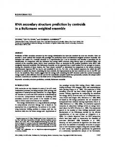
Ribonucleic acids (RNAs) are molecules that are responsible for regulating many genetic and metabolic activities in cells. An RNA is single-stranded and can be considered as a sequence of nucleotides (also known as bases). There are four basic nucleotides, namely, Adenine (A), Cytosine (C), Guanine (G), and Uracil (U). An RNA folds into a 3-dimensional structure by forming pairs of bases. Paired bases tend to stabilize the RNA (i.e., have negative free energy). Yet base pairing does not occur arbitrarily. In particular, A-U and C-G form stable pairs and are known as the Watson-Crick base pairs. Other base pairings are less stable and often ignored. An example of a folded RNA is shown in Figure 1. Note that this figure is just schematic; in practice, RNAs are 3-dimensional molecules. ∗

Department of Computer Science, Yale University, New Haven, CT 06520. Department of Computer Science, Northwestern University, Evanston, IL 60201 ([email protected]). This research was supported in part by NSF Grant EIA-0112934. ‡ Department of Computer Science, The University of Hong Kong, Hong Kong ({twlam, smyiu}@cs.hku.hk). This research was supported in part by Hong Kong RGC grant HKU-7027/98E. § Department of Computer Science, National University of Singapore, 3 Science Drive 2, Singapore 117543 ([email protected]). †

1

C C

C

A A

G

C

A A

G

A

U

U

A

A A

U

G

A

U

G G

A

A U

A U

Stacking Pair

U C G G

Hairpin Loop

U

U

G A

A

Internal Loop

C

C A

G

C G

U

Bulge

Multi-branched Loop

Figure 1: Example of a folded RNA The 3-dimensional structure is related to the function of the RNA. Yet existing experimental techniques for determining the 3-dimensional structures of RNAs are often very costly and time consuming (see, e.g., [6]). The secondary structure of an RNA is the set of base pairings formed in its 3-dimensional structure. To determine the 3-dimensional structure of a given RNA sequence, it is useful to determine the corresponding secondary structure. As a result, it is important to design efficient algorithms to predict the secondary structure with computers. From a computational viewpoint, the challenge of the RNA secondary structure prediction problem arises from some special structures called pseudoknots, which are defined as follows. Let S be an RNA sequence s1 , s2 , · · · , sn . A pseudoknot is composed of two interleaving base pairs, i.e., (si , sj ) and (sk , sℓ ) such that i < k < j < ℓ. See Figure 2 for examples. If we assume that the secondary structure of an RNA contains no pseudoknots, the secondary structure can be decomposed into a few types of loops: stacking pairs, hairpins, bulges, internal loops, and multiple loops (see, e.g., Tompa’s lecture notes [9] or Waterman’s book [11]). A stacking pair is a loop formed by two pairs of consecutive bases (si , sj ) and (si+1 , sj−1 ) with i + 4 ≤ j. See Figure 1 for an example. By definition, a stacking pair contains no unpaired bases and any other kinds of loops contain one or more unpaired bases. Since unpaired bases are destabilizing and have positive free energy, stacking pairs are the only type of loops that have negative free energy and stabilize the secondary structure. It is also natural to assume that the free energies of loops are independent. Then an optimal pseudoknot-free secondary structure can be computed using dynamic programming in O(n3 ) time [3, 5, 12, 13]. However, pseudoknots are known to exist in some RNAs. For predicting secondary structures with pseudoknots, Nussinov et al. [7] have studied the case where the energy function is minimized when the number of base pairs is maximized and have obtained an O(n3 )-time algorithm for predicting secondary structures. Based on some special energy functions, Lyngso and Pedersen [4] have proven that determining the optimal secondary

2

G

G G A

C

A

A

C

C U

U

U

U

G A A

G

C G

C

A

C

U

G

C

G

C

C

A

C

C

A

C

A

A

A

G

G

G

A

A

G

C

A

Figure 2: Examples of pseudoknots structure possibly with pseudoknots is NP-hard. Akutsu [1] has shown that it is NP-hard to determine an optimal planar secondary structure, where a secondary structure is planar if the graph formed by the base pairings and the backbone connections of adjacent bases is planar (see Section 2 for a more detailed definition). Rivas and Eddy [8], Uemura et al. [10], and Akutsu [1] have also proposed polynomial-time algorithms that can handle limited types of pseudoknots; note that the exact types of such pseudoknots are implicit in these algorithms and difficult to determine. Although it might be desirable to have a better classification of pseudoknots and better algorithms that can handle a wider class of pseudoknots, this paper approaches the problem in a different general direction. We initiate the study of predicting RNA secondary structures that allow arbitrary pseudoknots while maximizing the number of stacking pairs. Such a simple energy function is meaningful as stacking pairs are the only loops that stabilize secondary structures. We obtain two approximation algorithms with worst-case ratios of 1/2 and 1/3 for planar and general secondary structures, respectively. The planar approximation algorithm makes use of a geometric observation that allows us to visualize the planarity of stacking pairs on a rectangular grid; interestingly, such an observation does not hold if our aim is to maximize the number of base pairs. This algorithm runs in O(n3 ) time. The second approximation algorithm is more complicated and is based on a combination of multiple “greedy” strategies. A straightforward analysis cannot lead to the approximation ratio of 1/3. We make use of amortization over different steps to obtain the desired ratio. This algorithm runs in O(n) time. To complement these two algorithms, we also prove that allowing pseudoknots makes it NP-hard to find the planar secondary structure with the largest number of stacking pairs. The proof makes use of a reduction from a well-known NP-complete problem called Tripartite Matching [2]. This result indicates that the hardness of the RNA secondary structure prediction problem may be inherent in the pseudoknot structures and may not be necessarily due to the complication of the energy functions. This is in contrast to the other NP-hardness results discussed earlier. The rest of this paper is organized into four sections. Section 2 discusses some basic properties. Sections 3 and 4 present the approximation algorithms for planar and general secondary structures, respectively. Section 5 details the NP-hardness result. Section 6 concludes the paper with open problems.

3

2

Preliminaries

Let S = s1 s2 · · · sn be an RNA sequence of n bases. A secondary structure P of S is a set of Watson-Crick pairs (si1 , sj1 ), . . . , (sip , sjp ), where sir + 2 ≤ sjr for all r = 1, . . . , p and no two pairs share a base. We denote q (q ≥ 1) consecutive stacking pairs (si , sj ), (si+1 , sj−1 ); (si+1 , sj−1 ), (si+2 , sj−2 ) . . . (si+q−1 , sj−q+1 ), (si+q , sj−q ) of P by (si , si+1 , . . . , si+q ; sj−q , . . . , sj−1 , sj ). Definition 1 Given a secondary structure P, we define an undirected graph G(P) such that the bases of S are the nodes of G(P) and (si , sj ) is an edge of G(P) if j = i + 1 or (si , sj ) is a base pair in P. Definition 2 A secondary structure P is planar if G(P) is a planar graph. Definition 3 A secondary structure P is said to contain an interleaving block if P contains three stacking pairs (si , si+1 ; sj−1 , sj ), (si′ , si′ +1 ; sj ′ −1 , sj ′ ), (si′′ , si′′ +1 ; sj ′′ −1 , sj ′′ ) where i < i′ < i′′ < j < j ′ < j ′′ . Lemma 2.1 If a secondary structure P contains an interleaving block, P is non-planar. Proof. Suppose P contains an interleaving block. Without loss of generality, we assume that P contains the stacking pairs (s1 , s2 ; s7 , s8 ), (s3 , s4 ; s9 , s10 ), and (s5 , s6 ; s11 , s12 ). Figure 3(a) shows the subgraph of G(P) corresponding to these stacking pairs. Since this subgraph contains a homeomorphic copy of K3,3 (see Figure 3(b)), G(P) and P are non-planar. s3

s4 s2

s3 s1

s4

s5

s6

s9 s7

s2

s10

s11

s12

s1

s8 s6

s5

s7

s8

s12

s11

(a) s9

s10

(b)

Figure 3: Interleaving block

4

3

An Approximation Algorithm for Planar Secondary Structures

We present an algorithm which, given an RNA sequence S = s1 s2 . . . sn , constructs a planar secondary structure of S to approximate one with the maximum number of stacking pairs with a ratio of at least 1/2. This approximation algorithm is based on the subtle observation in Lemma 3.1 that if a secondary structure P is planar, the subgraph of G(P) which contains only the stacking pairs of P can be embedded in a grid with a useful property. This property enables us to consider only the secondary structure of S without pseudoknots in order to achieve 1/2 approximation ratio. Definition 4 Given a secondary structure P, we define a stacking pair embedding of P on a grid as follows. Represent the bases of S as n consecutive grid points on the same horizontal grid line L such that si and si+1 (1 ≤ i < n) are connected directly by a horizontal grid edge. If (si , si+1 ; sj−1 , sj ) is a stacking pair of P, si and si+1 are connected to sj and sj−1 respectively by a sequence of grid edges such that the two sequences must be either both above or both below L. Figure 4 shows a stacking pair embedding (Figure 4(b)) of a given secondary structure (Figure 4(a)). Note that (s3 , s9 ) do not form a stacking pair with other base pair, so s3 is not connected to s9 in the stacking pair embedding. Similarly, s4 is not connected to s10 in the embedding.

s3 s1

s4

s5

s9

s6 s7

s2

s10 s11

s12

s3

s8

s1

s4

s5

s9 s10

s6 s7

s2

s8

s11 s12

(b)

(a)

Figure 4: An example of a stacking pair embedding

Definition 5 A stacking pair embedding is said to be planar if it can be drawn in such a way that no lines cross or overlap with each other in the grid. The embedding shown in Figure 4(b) is planar. Lemma 3.1 Let P be a secondary structure of an RNA sequence S. Let E be a stacking pair embedding of P. If P is planar, then E must be planar.

5

Proof. If P does not have a planar stacking pair embedding, we claim that P contains an interleaving block. Let L be the horizontal grid line that contains the bases of S in E. Since P does not have a planar stacking pair embedding, we can assume that E has two stacking pairs intersect above L (see Figure 5(a)).

(a)

(d)

(g)

(b)

(c)

(e)

(f)

(h)

(i)

Figure 5: Non-planar stacking pair embedding If there is no other stacking pair underneath these two pairs, we can flip one of the pairs below L as shown in Figure 5(b). So, there must be at least one stacking pair underneath these two pairs. By checking all possible cases (all non-symmetric cases are shown in Figures 5(c) to (i)), it can be shown that E cannot be redrawn without crossing or overlapping lines only if it contains an interleaving block (Figures 5(h) and (i)). So, by Lemma 2.1, P is non-planar. By Lemma 3.1, we can relate two secondary structures having the maximum number of stacking pairs with and without pseudoknots in the following lemma. Lemma 3.2 Given an RNA sequence S, let N ∗ be the maximum number of stacking pairs that can be formed by a planar secondary structure of S and let W be the maximum number ∗ of stacking pairs that can be formed by S without pseudoknots. Then, W ≥ N2 . Proof. Let P ∗ be a planar secondary structure of S with N ∗ stacking pairs. Since P ∗ is planar, by Lemma 3.1, any stacking pair embedding of P ∗ is planar. Let E be a stacking pair embedding of P ∗ such that no lines cross each other in the grid. Let L be the horizontal grid line of E which contains all bases of S. Let n1 and n2 be the number of stacking pairs which are drawn above and below L, respectively. Without loss of generality, assume that n1 ≥ n2 . Now, we construct another planar secondary structure P from E by deleting all stacking pairs which are drawn below L. Obviously, P is a planar ∗ secondary structure of S without pseudoknots. Since n1 ≥ n2 , n1 ≥ N2 . As W ≥ n1 , ∗ W ≥ N2 .

6

Based on Lemma 3.2, we now present the dynamic programming algorithm M axSP which computes the maximium number of stacking pairs that can be formed by an RNA sequence S = s1 s2 . . . sn without pseudoknots. Algorithm M axSP Define V (i, j) (for j ≥ i) as the maximum number of stacking pairs without pseudoknots that can be formed by si . . . sj if si and sj form a Watson-Crick pair. Let W (i, j) (j ≥ i) be the maximum number of stacking pairs without pseudoknots that can be formed by si . . . sj . Obviously, W (1, n) gives the maximum number of stacking pairs that can be formed by S without pseudoknots. Basis: For j = i, i + 1, i + 2 or i + 3 (j ≤ n), V (i, j) = 0 W (i, j) = 0.

if si , sj form a Watson-Crick pair;

Recurrence: For j > i + 3,    V (i, j) W (i, j) = max W (i + 1, j)   W (i, j − 1) V (i, j)

= max

(

 if si , sj form a Watson-Crick pair    

;

V (i + 1, j − 1) + 1 if si+1 , sj−1 form a Watson-Crick pair maxi+1≤k≤j−2 {W (i + 1, k) + W (k + 1, j − 1)}

)

.

Lemma 3.3 Given an RNA sequence S of length n, Algorithm M axSP computes the maximum number of stacking pairs that can be formed by S without pseudoknots in O(n3 ) time and O(n2 ) space. Proof. There are O(n2 ) entries V (i, j) and W (i, j) to be filled. To fill an entry of V (i, j), we check at most O(n) values. To fill an entry of W (i, j), O(1) time suffices. The total time complexity for filling all entries is O(n3 ). Storing all entries requires O(n2 ) space. Although Algorithm M axSP presented in the above only computes the number of stacking pairs, it can be easily modified to compute the secondary structure. Thus we have the following theorem. Theorem 3.4 The Algorithm M axSP is an (1/2)-approximation algorithm for the problem of constructing a secondary structure which maximizes the number of stacking pairs for an RNA sequence S.

7

4

An Approximation Algorithm for General Secondary Structures

We present Algorithm GreedySP () which, given an RNA sequence S = s1 s2 . . . sn , constructs a secondary structure of S (not necessarily planar) with at least 1/3 of the maximum possible number of stacking pairs. The approximation algorithm uses a greedy approach. Figure 6 shows the algorithm GreedySP (). // Let S = s1 s2 . . . sn be the input RNA sequence. Initially, all sj are unmarked. // Let E be the set of base pairs output by the algorithm. Initially, E = ∅. GreedySP (S, i)

// i ≥ 3

1. Repeatedly find the leftmost i consecutive stacking pairs SP (i.e., find (sp , . . . , sp+i ; sq−i , . . . , sq ) such that p is as small as possible) formed by unmarked bases. Add SP to E and mark all these bases. 2. For k = i − 1 downto 2, Repeatedly find any k consecutive stacking pairs SP formed by unmarked bases. Add SP to E and mark all these bases. 3. Repeatedly find the leftmost stacking pair SP formed by unmarked bases. Add SP to E and mark all these bases. Figure 6: A 1/3-Approximation Algorithm In the following, we analyze the approximation ratio of this algorithm. The algorithm GreedySP (S, i) will generate a sequence of SP ’s denoted by SP1 , SP2 , . . . , SPh . Fact 4.1 For any SPj and SPk (j 6= k), the stacking pairs in SPj do not share any base with those in SPk . For each SPj = (sp , . . . , sp+t ; sq−t , . . . , sq ), we define two intervals of indexes, Ij and Jj , as [p..p + t] and [q − t..q], respectively. In order to compare the number of stacking pairs formed with that in the optimal case, we have the following definition. Definition 6 Let P be an optimal secondary structure of S with the maximum number of stacking pairs. Let F be the set of all stacking pairs of P. For each SPj computed by GreedySP (S, i) and β = Ij or Jj , let Xβ = {(sk , sk+1 ; sw−1 , sw ) ∈ F| at least one of indexes k, k + 1, w − 1, w is in β}. Note that Xβ ’s may not be disjoint. Lemma 4.2

S

1≤j≤h {XIj

∪ XJj } = F.

Proof. We prove this lemma by contradiction. Suppose that there exists a stacking pair (sk , sk+1 ; sw−1 , sw ) in F but not in any of XIj and XJj . By Definition 6, none of the 8

indexes, k, k + 1, w − 1, w is in any of Ij and Jj . This contradicts with Step 3 of Algorithm GreedySP (S, i). Definition 7 For each XIj , [ [ let XI′ j = XIj − {XIk ∪ XJk }, and let XJ′ j = XJj − {XIk ∪ XJk } − XIj k 0. The following lemma shows a property of delimiter fragments in open regions. Lemma 5.5 If Sj is an open region, then both delimiter fragments of either Vj or Wj must not pair with their conjugate fragments in OPT. Proof. We prove the statement by contradiction. Suppose one fragment of Vj and one fragment of Wj are paired with their conjugate fragments. Let (sx , sx+1 ; sy−1 , sy ) and (sx′ , sx′ +1 ; sy′ −1 , sy′ ) be some particular stacking pairs in Vj and Wj , respectively. Since Sj is an open region, we can identify a stacking pair (sx′′ , sx′′ +1 ; sy′′ −1 , sy′′ ) where sx′′ sx′′ +1 and sy′′ −1 sy′′ are 2-substrings within and outside Sj , respectively. Note that these three stacking pairs form an interleaving block. By Lemma 2.1, OPT is not planar, reaching a contradiction. 5.3.3

Proof of the only-if part

By Lemma 5.4, it suffices to assume that Sm+1 is an open region. Before we give the proof of the only-if part, let us consider the following lemma. Lemma 5.6 Let α be the number of delimiter fragments that are not paired with their conjugate fragments. Then, ♦CC + ♦GG ≥ α + (#GC − ♦GC). Proof. By construction, a GC-substring must be next to the left end of a delimiter fragment F , which is of the form C + . No other GC-substrings can exist. If this GC-substring is paired, the leftmost CC-substring of F must not be paired as there is no GGC pattern in SE . Thus, F must be one of the α delimiter fragments that are not paired with their conjugate fragments. Based on this observation, we classify the α delimiter fragments into 15

two groups: (1) (#GC − ♦GC)’s delimiter fragments whose GC-substrings at the left end are paired; and (2) α − (#GC − ♦GC)’s delimiter fragments whose GC-substrings at the left end are not paired. For each delimiter fragment F = C 2d+k in group (1), since the GC-substring on the left of F is paired, the leftmost CC-substring of F must not be paired by OPT. For the remaining 2d + k − 2 CC-substrings, we either find a CC-substring which is not paired by OPT; or these 2d + k − 2 CC-substrings are paired to GG-substrings in some fragment ′ F ′ = G2d+k with 2d > k′ > k, and thus, some GG-substring of F ′ is not paired. Therefore, each delimiter fragment in group (1) introduces either (i) two unpaired CC-substrings or (ii) one unpaired CC-substring and one unpaired GG-substring. Hence, the total number of unpaired CC and GG-substrings due to delimiter fragments in group (1) ≥ 2(#GC −♦GC). For each delimiter fragment F = C 2d+k in group (2), consider the CC-substrings in F . With a similar argument, we can show that each delimiter fragment in group (2) introduces either (i) one unpaired CC-substring or (ii) one unpaired GG-substring. Hence, the total number of unpaired CC and GG-substrings due to delimiter fragments in group (2) ≥ α − (#GC − ♦GC). In total, we have ♦CC + ♦GG ≥ α + (#GC − ♦GC). Now, we state a lemma which shows the lower bounds for some ♦ values in terms of the number of open regions in OPT. Lemma 5.7 Let ℓ ≥ 1 be the number of open regions in OPT. (1) If Sm+1 is an open region, then ♦U U ≥ 3(m + 1 − ℓ)d. (2) max{♦CC, ♦GG} ≥ ℓ + (#GC − ♦GC)/2. (3) If ℓ = n + 1, Sm+1 is an open region, and E does not have a perfect matching, then either (a) ♦U U ≥ 3(m − n)d + 1, (b) ♦AA ≥ 1, or (c) ♦U A ≥ 2. Proof. Statement 1. Within each closed region Sj where j 6= m + 1, 3d’s U U -substrings cannot

paired in OPT. As there are m + 1 − ℓ such closed regions, 3(m + 1 − ℓ)d U U -substrings are not paired in OPT. Thus, ♦U U ≥ 3(m + 1 − ℓ)d. Statement 2. By Lemma 5.5, we can identify 2ℓ fragments in Vj and Wj of all open

regions which are not paired with their conjugate fragments. Then, by Lemma 5.6, we have ♦CC + ♦GG ≥ 2ℓ + (#GC − ♦GC). Thus, max{♦CC, ♦GG} ≥ ℓ + (#GC − ♦GC)/2. Statement 3. By a similar argument to the proof for Statement 1, within the m + 1 − ℓ =

m − n closed regions, 3(m − n)d U U -substrings are not paired in OPT. For the ℓ = n + 1 open regions, one of them must be Sm+1 . Let Sj1 , . . . , Sjn be the remaining n open regions. Recall that ej1 , . . . , ejn are the corresponding edges of these n open regions. Since these n edges cannot form a perfect matching, some node, says xk , is adjacent to these n edges more than once. Thus, within Sj1 , . . . , Sjn , Sm+1 , we have more hxk i than hxk i. Therefore, at least two of the fragments in all hxk i are not paired with their conjugate fragments.

16

Let F be one of such fragments. Note that F is of the form U d Ak . Since F is not paired with its conjugate fragment, one of the following three cases occurs in OPT: Case 1: An U U -substring of F is not paired. Case 2: An AA-substring of F is not paired. Case 3: All U U -substrings and AA-substrings F are paired. In this case, U d of F is paired ′ with Ad of a fragment F ′ = U k Ad ; and Ak of F is paired with some substring U k of some fragment F ′′ . As F ′ and F ′′ are not the same fragment, the U A-substrings of both F and F ′ are not paired. In summary, we have either (1) ♦U U ≥ 3(m−n)d+1, or (2) ♦AA ≥ 1, or (3) ♦U A ≥ 2. Based on Lemma 5.7, we prove the only-if part by a case analysis in the following lemma. Lemma 5.8 If E does not have a prefect matching, then #OPT < h. Proof. Recall that if Sm+1 is a closed region, then #OPT < h. Now, suppose that Sm+1 is an open region. We show #OPT < h in three cases ℓ < n + 1, ℓ > n + 1 and ℓ = n + 1. Case 1: ℓ < n + 1. By Lemma 5.7 (1), ♦U U ≥ 3(m + 1 − ℓ)d. By Fact 5.3, we can conclude that #OPT = h + n + 1 + (2m + 2) − 3(n + 1 − ℓ)d ≤ h + n + 1 + (2m + 2) − 3d < h. Case 2: ℓ > n + 1. By Lemma 5.7 (2), max{♦CC, ♦GG} ≥ ℓ + (#GC − ♦GC)/2. By Fact 5.3, #OPT ≤ h + n + 1 − ℓ, which is smaller than h because ℓ > n + 1. Case 3: ℓ = n + 1. By Lemma 5.7 (3), either (a) ♦U U ≥ 3(m − n)d + 1, or (b) ♦AA ≥ 1, or (c) ♦U A ≥ 2. By Fact 5.3, #OPT ≤ h + n − max{♦CC, ♦GG} + (#GC − ♦GC)/2. By Lemma 5.7 (2), we have #OPT < h. We conclude that if E does not have a prefect matching, then #OPT < h. Equivalently, if #OPT ≥ h, then E has a prefect matching.

6

Conclusions

In this paper, we have studied the problem of predicting RNA secondary structures that allow arbitrary pseudoknots with a simple free energy function that is minimized when the number of stacking pairs is maximized. We have proved that this problem is NP-hard if the secondary structure is required to be planar. We conjecture that the problem is also NP-hard for the general case. We have also given two approximation algorithms for this problem with worst-case approximation ratios of 1/2 and 1/3 for planar and general secondary structures, respectively. It would be of interest to improve these approximation ratios. Another direction is to study the problem using energy function that is minimized when the number of base pairs is maximized. It is known that this problem can be solved in cubic time if the secondary structure can be non-planar [7]. However, the computational complexity of the problem is still open if the secondary structure is required to be planar. We conjecture that the problem becomes NP-hard under this additional condition. We

17

would like to point out that the observation that have enabled us to visualize the planarity of stacking pairs on a rectangular grid does not hold in case of maximizing base pairs.

References [1] T. Akutsu. Dynamic programming algorithms for RNA secondary structure prediction with pseudoknots. Discrete Applied Mathematics, 104(1-3):45–62, 2000. [2] M. Garey and D. Johnson. Computers and Intractability: A Guide to the Theory of NP-Completeness. Freeman, New York, NY, 1979. [3] R. Lyngsø, M. Zuker, and C. Pedersen. Internal loops in RNA secondary structure prediction. In Proceedings of the 3rd Annual International Conference on Computational Molecular Biology, pages 260–267, Lyon, France, 1999. [4] R. B. Lyngsø and C. N. S. Pedersen. RNA pseudoknot prediction in energy based models. Journal of Computational Biology, 7(3/4):409–428, 2000. [5] R. B. Lyngsø, M. Zuker, and C. N. S. Pedersen. Fast evaluation of internal loops in RNA secondary structure prediction. Bioinformatics, 15(6):440–445, 1999. [6] J. Meidanis and J. Setubal. Introduction to Computational Molecular Biology. International Thomson Publishing, New York, 1997. [7] R. Nussinov, G. Pieczenik, J.R. Griggs, and D.J. Kleitman. Algorithms for loop matchings. SIAM Journal on Applied Mathematics, 35(1):68–82, 1978. [8] E. Rivas and S. R. Eddy. A dynamic programming algorithm for RNA structure prediction including pseudoknots. Journal of Molecular Biology, 285(5):2053–2068, 1999. [9] M. Tompa. Lecture notes on biological sequence analysis. Technical Report #200006-01, Department of Computer Science and Engineering, University of Washington, Seattle, 2000. [10] Y. Uemura, A. Hasegawa, S. Kobayashi, and T. Yokomori. Tree adjoining grammars for RNA structure prediction. Theoretical Computer Science, 210(2):277–303, 1999. [11] M. S. Waterman. Introduction to Computational Biology: Maps, Sequences and Genomes. Chapman & Hall, New York, NY, 1995. [12] M. Zuker. The use of dynamic algorithms in RNA secondary structure prediction. In M. S. Waterman, editor, Mathematical Methods for DNA Sequences, pages 159–184. CRC Press Inc., Boca Raton, FL, 1989. [13] M. Zuker and D. Sankoff. RNA secondary structures and their prediction. Bulletin of Mathematical Biology, 46(4):591–621, 1984.

18