SILVA FENNICA. Silva Fennica 43(3) research articles ... E-mail matti.maltamo(at)joensuu.fi ... Available at http://www.metla.fi/silvafennica/full/sf43/sf433507.pdf ...
SILVA FENNICA
Silva Fennica 43(3) research articles www.metla.fi/silvafennica · ISSN 0037-5330 The Finnish Society of Forest Science · The Finnish Forest Research Institute
Predicting Tree Attributes and Quality Characteristics of Scots Pine Using Airborne Laser Scanning Data Matti Maltamo, Jussi Peuhkurinen, Jukka Malinen, Jari Vauhkonen, Petteri Packalén and Timo Tokola
Maltamo, M., Peuhkurinen, J., Malinen, J., Vauhkonen, J., Packalén, P. & Tokola, T. 2009. Predicting tree attributes and quality characteristics of Scots pine using airborne laser scanning data. Silva Fennica 43(3): 507–521. The development of airborne laser scanning (ALS) during last ten years has provided new possibilities for accurate description of the living tree stock. The forest inventory applications of ALS data include both tree and area-based plot level approaches. The main goal of such applications has usually been to estimate accurate information on timber quantities. Prediction of timber quality has not been focused to the same extent. Thus, in this study we consider here the prediction of both basic tree attributes (tree diameter, height and volume) and characteristics describing tree quality more closely (crown height, height of the lowest dead branch and sawlog proportion of tree volume) by means of high resolution ALS data. The tree species considered is Scots pine (Pinus sylvestris), and the field data originate from 14 sample plots located in the Koli National Park in North Karelia, eastern Finland. The material comprises 133 trees, and size and quality variables of these trees were modeled using a large number of potential independent variables calculated from the ALS data. These variables included both individual tree recognition and area-based characteristics. Models for the dependent tree characteristics to be considered were then constructed using either the non-parametric k-MSN method or a parametric set of models constructed simultaneously by the Seemingly Unrelated Regression (SUR) approach. The results indicate that the k-MSN method can provide more accurate tree-level estimates than SUR models. The k-MSN estimates were in fact highly accurate in general, the RMSE being less than 10% except in the case of tree volume and height of the lowest dead branch. Keywords alpha shape, crown height, height metrics, k-MSN, lidar, timber quality Addresses Maltamo, Peuhkurinen, Vauhkonen, Packalén and Tokola, University of Joensuu, Faculty of Forest Sciences, FI-80101 Joensuu, Finland; Malinen, Finnish Forest Research Institute, Joensuu Research Unit, FI-80101 Joensuu, Finland E-mail matti.maltamo(at)joensuu.fi Received 28 May 2008 Revised 17 December 2008 Accepted 28 January 2009 Available at http://www.metla.fi/silvafennica/full/sf43/sf433507.pdf
507
Silva Fennica 43(3), 2009
1 Introduction Quality assessments of trees have rarely been carried out in traditional forest inventories where stands have usually been characterised by registering species and measuring tree diameters and heights. Variables that are more closely related to the external technical quality of trees, such as branch height characteristics and actual sawlog recovery, i.e. sawlog recovery in the light of technical defects and bucking constraints, have been measured or assessed only in specific inventories or from sample trees, since these measurements have been found to be too laborious in practice. Thus the forest resource data used for planning purposes for example in Finland, do not include detailed information on tree quality. The description of the quality of tree stock is, however, of primary interest. Information on quality can be used when selecting stands to be bought and what kind of end-use they are suitable. Tree stock quality together with market situation affects on decision of harvesting schedule from where timber should be cut in order to fulfil production demands. If quality characteristics of marked stands are not known considerable economical losses may arise. The development of high resolution remote sensing techniques has made it possible to obtain tree-level information. In the case of 2D data, usually in the form of aerial photographs, such information is restricted to characteristics related to the area of the tree crown, but tree height can also be assessed when using 3D data. The most commonly used 3D information is based on airborne laser scanning (ALS), which also provides information on tree crowns and stems by means of spatially registered (3D) point measurements of the canopy. ALS data have been used for many forestry purposes in recent years, including the prediction of mean stand characteristics (Næsset 1997), pre-harvest inventories (Peuhkurinen et al. 2007), comparisons of forest inventories based on cost plus loss analysis (Eid et al. 2004), ecological studies (Omasa et al. 2003, Gaveau and Hill 2003) and assessments of forest growth issues (Yu et al. 2004). In general, ALS data can be utilized both on individual tree level and per area unit. The accu508
research articles
racy of stand level estimates (volume, basal area, stem number, mean height and diameter) from area based forest inventories using ALS is usually very good (see Næsset et al. 2004, Packalén and Maltamo 2007). In such approaches the height information in the ALS point data is used to predict the forest variables statistically. Such an area based approach was for example used by Korhonen et al. (2008) to estimate stand sawlog recovery rates. More detailed information on detected trees can be obtained when ALS data are used at the tree level, although only a proportion of the individual trees in the standing stock can be detected in this way and a model chain is needed to derive forest inventory end products (Persson et al. 2002, Maltamo et al. 2004a, 2007, Solberg et al. 2006). Since the proportion of trees detected varies according to the stand density, spatial pattern and tree species, it has been quite difficult to obtain general forest resource information by means of individual tree approaches. Nevertheless, the use of ALS data at the individual tree level offers possibilities for obtaining information on the quality of the trees detected. Estimates of crown height (lower limit of the continuous living crown) have been obtained using ALS-based tree level statistical models (Næsset and ∅kland 2002, Maltamo et al. 2006a, Popescu and Zhao 2008). Peuhkurinen et al. (2007) successfully retrieved pre-harvest quality information of marked stands from ALS data. The recognition of trees and prediction of their diameters was highly accurate in sparsely stocked stand. In the final phase, timber assortments were calculated using taper curves and the results were compared with accurately measured harvester data. Tree-level and area-based ALS variables can be combined in tree level prediction models. Examples of such processes have involved tree crown height prediction (Næsset and ∅kland 2002, Maltamo et al. 2006a), species interpretation (Holmgren and Persson 2004), and stem volume modelling (Takahashi et al. 2005, Chen et al. 2007, Villikka et al. 2007). ALS data also provide possibilities for deriving 3D texture variables for tree crowns. Vauhkonen et al. (2008) employed the alpha shape concept, a computational geometry technique introduced by Edelsbrunner and Mücke (1994), to construct tree
Maltamo, Peuhkurinen, Malinen, Vauhkonen, Packalén and Tokola
crown approximations from ALS point clouds. They used this information to predict tree species, although it could equally well be used to determine tree crown variables (Vauhkonen 2008). This study aimed at developing a method of utilizing ALS data for determination of certain tree-level characteristics, with specific focus on external tree quality. The characteristics considered were tree diameter, height, volume, crown height, height of the lowest dead branch and actual sawlog proportion of stem volume, i.e. the proportion of the volume which meets the dimension and quality requirements for sawlogs. The tree species considered was Scots pine (Pinus sylvestris) and the material was restricted to sawlog-sized trees. Both tree level and area based ALS derived variables were used in the current models. A non-parametric k-MSN method and a parametric set of models constructed simultaneously by the Seemingly Unrelated Regression (SUR) approach were compared and appraised on the basis of mean prediction error and RMSE estimates.
2 Material and Pre-Processing A test site was chosen in the southern part of the Koli National Park in North Karelia, eastern Finland, and 14 rectangular plots were established there during the spring of 2006. These were typically located in randomly chosen pure Scots pine stands on poor soils. To have around 100 trees per plot, quadratic plots of 30 by 30 meters were established. All trees with a diameter at breast height (DBH) of more than 5 cm were mapped and the species, height, crown height (LCH), DBH and diameter at a height of 6 metres (D6) were recorded for each. Sawlog-sized Scots pines (DBH over 17 cm) were selected for the study of a number of external technical quality variables, as presented and defined in Table 1. In addition, sawlog proportion of stem volume was calculated for all the sawlog-sized Scots pines using the following criteria
Predicting Tree Atributes and Quality Characteristics of Scots Pine … – maximum diameter of a living branch < 60 mm, – maximum curvature or crookedness < 1cm within 1 metre, – no curves in the crown part or multiple curvature, and – no other defects such as decay, worm holes, cracks or foreign objects.
Sawlogs as a proportion of stem volume was then calculated as the volume of that part of the tree that fulfilled the above requirements using the taper curve models of Laasasenaho (1982). Total stem volumes (V) were calculated using the stem volume models of Laasasenaho (1982), which include tree height, DBH and D6 as independent variables. Altogether there were 929 living Scots pine trees, of which 449 were of sawlog size. Differentially corrected Global Positioning System measurements with an accuracy of approximately 1 metre in the XY directions were used to determine the position of the four corners of each of the 14 plots. This accuracy is based on measurements using Real Time Kinematic technique, static GPS and tachymeter measurements in the same area. Tree locations within a plot were assessed by projecting the trees onto the same coordinate system as in the ALS data by affine transformation using the measured corner positions as reference points. Georeferenced ALS point cloud data were collected from an area of approximately 2500 hectares in Koli on July 13 2005 using an Optech ALTM 3100 scanner operated at a mean altitude of 900 m above ground level, resulting in a nominal sampling density of about 4 points per m2. Elevation within the test area varied from 95 m to 350 m (local zero sea level), resulting in a varying sampling density across the target. The divergence of the laser beam (1064 nm) was 0.26 mrad. The data were captured using a scanning angle of ±11 degrees, which resulted in a swath width of about 350 m. The last pulse data were employed to generate a digital terrain model (DTM) by the method explained in Axelsson (2000), using a grid size of 1 m.
– log length > 310 cm, – DBH > 170 mm, – maximum diameter of a dead or vertical branch < 40 mm,
509
Silva Fennica 43(3), 2009
research articles
Table 1. Definitions of tree quality variables. Quality variable
Definition
Crown height
The height of the lower limit of the continuous living crown, which is defined as beginning from the height above which all branches will be dead after a maximum of one year’s successive growth period
Height of the lowest dead branch
The height of the lowest dead branch of diameter > 15 mm
Height of the largest living branch
Height of the dead branch with largest diameter
Height of the largest dead branch
Height of the dead branch with largest diameter
Oversized living branch
Height of an oversized living branch (diameter > 60 mm) not acceptable for sawlogs
Oversized dead branch
Height of an oversized dead branch (diameter > 40 mm) not acceptable for sawlogs
Other defect
Height of some other defect that affects the external technical quality of the timber (decay, dead crown, etc.)
3 Methodology 3.1 Identification of Individual Trees Terrain surface heights (i.e. vegetation heights) for the laser points were obtained by subtracting the corresponding DTM values. Points with a value over 0.5 m were classified as vegetation hits (see Hyyppä and Inkinen 1999). The Canopy Height Model (CHM) was interpolated to a regular grid of 0.5 m using canopy heights by taking the maximum value of the laser measurements within a radius of 0.5 m. Because the ALS point cloud is not exactly regular, the method is not able to produce a value for every grid cell (pixel). Consequently values for the missing pixels (pixels with no value) were interpolated by taking the average from a 3 × 3 pixel window in each case and performing the interpolations successively until every pixel had a value. The CHM was low-pass filtered using the Gaussian kernels, as in the method suggested by Pitkänen et al. (2004), where the size of the filtering window and the intensity of the filtering were increased stepwise as a function of the heights of the CHM. The size of the window is smallest and the filtering mildest in the lowest class, while correspondingly, the filtering is always the 510
most intense at the highest level of heights. The parameters required in the height-based filtering include a sigma (σ) and corresponding height classes. The height ranges and their ơ values were 0–8 m ơ 0.4; 8–16 m ơ 0.6; 16–24 m ơ 0.8; 24–32 m ơ 1.0; 32–40 m ơ 1.2. Local height maxima were searched for in the low-pass filtered CHM by a method in which all the pixels are first marked as possible maxima (Pitkänen et al. 2004), after which all those having a neighbour in an eight-connected neighbourhood with a greater value than the pixel itself were labelled as non-maxima. Thirdly, local maxima were found in the highest sections of the CHM and also in the lowest sections (ground), the former being finally taken to represent tree tops, whereas the latter were masked out by a binarization process in which all the pixels were classified as belonging either to the tree canopy or to the background area by defining a threshold value. This value was set at 2 metres to guarantee that all the trees measured (DBH at least 5 cm) could be found and to eliminate the undergrowth from the local maxima in the background area. The filtered CHM was segmented by watershed segmentation using a flooding algorithm following the direction of drainage (Gauch 1999, Pitkänen 2005). In watershed segmentation an
Maltamo, Peuhkurinen, Malinen, Vauhkonen, Packalén and Tokola
Predicting Tree Atributes and Quality Characteristics of Scots Pine …
Table 2. Characteristics of the trees identified (n=133), as measured in the field. Characteristic
Stem volume, m3 Proportion of sawlogs Diameter at breast height, cm Height, m Crown height, m Height of the lowest dead branch, m
Mean
Maximum
Minimum
Standard deviation
0.448 0.756 24.23 19.52 11.14 5.00
1.186 0.958 37.60 27.20 18.80 11.30
0.140 0.309 17.20 12.10 4.80 0.30
0.234 0.145 4.65 3.67 3.05 2.45
image is regarded as a topographic surface where the darkest z values represent low points and the brightest ones the highest points and is visualized in three dimensions: x- and y- and z-coordinates (Gonzales and Woods 2002). Starting from the minimum values of the image, the surface is then filled with water. To avoid merging basins, dams consisting of single pixels are built around their edges. Finally, all the basins are bounded by dams, which thus constitute the boundaries of the segments (Beucher 1992, Gonzales and Woods 2002). The watershed algorithms produce closed boundaries, even though the transitions between areas are not equally strong (Adams and Bischof 1994). The algorithm used here processed the negative of the CHM and the segmentation was started from the local minima, which were actually the local maxima of the CHM, i.e. the assumed tops of the canopies. Pixels belonging to the local minima were labelled with a new segment number, whereas those not belonging to the minima were linked to their neighbouring pixels with the smallest value. Every pixel was linked to one minimum by following the path thus formed. The flooding algorithm was then followed through. Finally, the binarization and segmentation processes were combined and those pixels which were labelled as background in the thresholding were also set as background in the segmentation image. Thus the canopy segments did not include any pixels with a height value smaller than the threshold value (2 metres), and no local maxima outside the canopy were taken into account. The procedure resulted in 687 canopy segments, which were taken as automatically detected candidate trees. The segments were then linked to field trees a) if there existed only one field tree inside the segment, and b) if the difference between the
maximum pulse height value in the segment and the height of the field tree was less than 2 metres. The linked trees were considered to be correctly identified and it is these that were selected for further analysis. This process of linking the candidate trees to field trees resulted in a total of 185 correctly identified trees, of which 133 were of sawlog size. The characteristics of these trees are presented in Table 2. 3.2 Derived ALS Characteristics The modelling of DBH, height, volume, crown height, height of the lowest dead branch and the proportion of sawlogs involved the calculation of various ALS-based characteristics at both the tree and plot level. These characteristics included physical tree variables, tree and plot-level ALS point cloud characteristics, alpha shape variables and indices of spatial competition. The calculation of these variables will be explained below. Even though the Optech ALTM 3100 records up to four echoes per pulse, we only used “first” and “last” echoes where the original “only” echoes were duplicated to both of these pulse classes. The so called “intermediate” echoes were not used. The height distributions of the first and last pulse canopy height hits was used to calculate plot-level percentiles for 0, 1, 5, 10, 20, …, 90, 95, 99 and 100% heights (H0, H1, H5, H10,…, H100) (see Næsset 2002), and cumulative proportional canopy densities (P0, P1, P5, P10,…, P100) were calculated for the respective deciles. The height distributions contained only those laser points which were classified as above-ground hits, using a threshold value of 0.5 metres. H5, for example, denotes the height at which the accumulation of laser hit heights in the vegetation is 5%, and 511
Silva Fennica 43(3), 2009
correspondingly, P5 denotes the proportion of laser hits accumulating at the 5% height. Other variables calculated for the sample plots were the proportion of ground hits versus canopy hits, using a threshold value of 0.5 metres (VEG), and the average height (Hmean) and standard deviation of the above ground hits (Hstd). All the metrics were calculated separately for both the first (F) and last pulse data (L). After the tree segmentation, ALS based estimates of tree height (hALS), crown area (acrALS), maximum crown diameter (dcrmaxALS), crown diameter perpendicular to the maximum crown diameter (dcrperpALS) and mean crown diameter (dcrmeanALS) were derived. hALS is equal to the elevation of the highest ALS point within a crown. The tree crown areas and diameters were extracted from the tree segments in the ALS data. The corresponding height metrics (heights h and densities p) were calculated for the areas of identified trees as in the case of the plot-level data, in addition to which estimates for the length (lbALS) and height of the longest branch (hbALS) were calculated from the ALS point cloud data Different computational geometry techniques were employed for deriving the other crown characteristics. The estimate for crown height (LCHALS) was based on calculating the crosssectional area, defined as the convex hull of the point data, at different heights. The maximum area of the point cloud was first calculated and the point cloud was then traversed from the 20% tree height towards the top. The area that included the traversed point was then calculated and the crown base at the point where the area calculated in this way exceeded a threshold of 20% of the maximum area was defined. This threshold was based on empirical tests. A 3D alpha shape (Edelsbrunner and Mücke 1994) was constructed from the points above this crown base. An alpha shape can be regarded as a weighted Delaunay triangulation from which all the simplices which have an empty circumsphere with a squared radius larger than the defined alpha value have been removed, i.e. the alpha value determines the level of detail in the shape obtained. Here the traversing of alpha values (Vauhkonen et al. 2008) was avoided by performing the computation using an optimal alpha value (opt_alpha) selected such that the resulting alpha shape included all the data points 512
research articles
within a single connected component. The volume of the interior (int_vol) and exterior (ext_vol) of the alpha shape were extracted for estimating the size and shape of the tree crown. Finally, in the case of individual tree detection, the location and height of each detected tree was obtained together with the same characteristics for neighbouring trees. This allowed us to calculate height-based competition indices. The local maxima of the tree segment were taken as the tree top locations. Using this spatial information, additive competition indices were calculated for all the individually detected trees. The calculated competition indices were based on elevation angle sums (Miina and Pukkala 2000) and were calculated using the equation n h −a×h CI a _ b = ∑ arctan i (1) di i =1 where CIa_b = competition index of the target tree, a = relative height of the horizontal plane (relative to the height of the target tree), b defines the maximum distance for a tree i to be regarded as a competitive tree, h = height of the target tree, d = horizontal distance between the spatial locations of the target tree and neighbouring trees i and i = competitive tree within a distance in maximum b to the target tree. Parameter a defines what trees are competitive trees based on the heights of the trees and how competitive the neighbouring trees are as a function of the vertical distance between the trees. Only trees with heights greater than the height of the horizontal plane are regarded as competitive trees. The competition indices for the correctly identified trees were calculated taking all the candidate trees as potential competitors and using different values for a and b. 3.3 The k-MSN Method The k-MSN method is a non-parametric method which uses canonical correlation analysis to produce a weighting matrix used for the selection of the k Most Similar Neighbours from reference data. Most Similar Neighbours are observations that according to predictor variables are similar to the target of prediction (Moeur and Stage 1995). By using canonical correlations it is possible to find the linear transformations Uk and Vk of the
Maltamo, Peuhkurinen, Malinen, Vauhkonen, Packalén and Tokola
set of dependent variables (Y, tree variables) and independent variables (X, ALS variables) which maximize the correlation between them: U k = α kY , and Vk = γ k X
D 2uj = (X u − X j ) ΓΛ 2 Γ' (X u − X j )′ p× p
n
RMSE =
∑ ( y − yˆ ) i =1
i
2
i
n
(2)
where αk is the canonical coefficient of the independent variables and γk is the canonical coefficient of the dependent variables. The MSN distance metric derived from canonical correlation analysis is: 1× p
Predicting Tree Atributes and Quality Characteristics of Scots Pine …
(3)
p ×1
where Xu is the vector of the known search variables from the target observation, Xj is the vector of the search variables from the reference observation, Γ is the matrix of canonical coefficients of the predictor variables and Λ is the diagonal matrix of squared canonical correlations. To optimize the accuracy of estimates produced using the derived model a variable subset selection method was used that is based on an optimization algorithm which inserts transformations x = x2, x = x , x = 1/x and x = log(x) of the predictor variables and removes all the variables via stepwise optimization of the relative RMSE of volume (Maltamo et al. 2006b). The insertion and deletion phases are conducted twice. 3.4 SUR Models The response variables were also simultaneously modeled by means of Seemingly Unrelated Regression (SUR) (Zellner 1962; Borders 1989). SUR models were estimated using the R-software (R Development Core Team 2007), the candidate models having first been constructed by OLS estimation and stepwise predictor selection. 3.5 Accuracy Assessment Accuracy was assessed by cross-validation, where observations from the same plot were not used in the estimation stage. The results were validated in terms of absolute and relative RMSE and absolute mean prediction error at the tree level:
(4) n
mean prediction error =
∑ ( y − yˆ ) i =1
i
n
i
(5)
where n is the number of trees, yi is the observed value for tree i and yˆi is the predicted value for tree i. The relative RMSEs were calculated by dividing the absolute values by the means of the observed variables. The usability of the ALS-based estimates was also tested by calculating estimates for further tree variables based on the characteristics modelled. These variables were slenderness (height /DBH), form factor (volume /(basal area × height)), crown ratio ((height-crown height)/height) and length of the dead branch section (crown height-height of the lowest dead branch).
4 Results There were usually 20–30 predictors and their transformations in the k-MSN models, similar to the results reported by Packalén and Maltamo (2007). The dependent variable and its squared transformations were always used in the canonical correlation analysis. An example of the predictor variables used in modelling the sawlog proportion is presented in Table 3. The SUR models for the tree and quality variables considered here (Table 4), contained only 2–6 predictors. Tree height, for example, was not used as a predictor when modelling DBH. Correspondingly, it is worth noting that the plot-level characteristics and ALS-based longest branch explained best the variation in height of the lowest dead branch. The RMSE and mean prediction error of the height estimates derived directly from the ALS data (hALS) were 0.74 m and 0.56 m, respectively, while the ALS-based estimate of crown height had an RMSE and mean prediction error of 2.1 m and –0.87 m, respectively. The accuracies of the variables derived from the models are presented in Table 5. As the table shows the k-MSN estimates 513
Silva Fennica 43(3), 2009 1.4
A
research articles
k MSN
1.2
SUR
1.1
Estimate
Estimate
0.9
0.8
0.6
0.5 0.5 15
0.8
Reference
1.1
1.4
0.8
0.6
Reference
0.9
1.2
D
0.6
Estimate
Estimate
0.3 0.3
C
10
0.4
5
0
B
0
5
Reference
10
15
0.2 0.2
0.4
Reference
0.6
0.8
Fig. 1. Derived tree characteristics: A – tree slenderness, B – form factor, C – length of dead branch section, and D – crown ratio.
seem to be more reliable than the SUR estimates. There are also notable differences between the volume and branch height characteristics in terms of relative RMSE. The number of nearest neighbours (k) used varied from two to eight, being eight in the case of most variables. The ALS-based estimates of slenderness, form factor, crown ratio and the length of the dead branch section are presented in Fig. 1, which again shows the better accuracy of the k-MSN estimates. The form factor was estimated substantially less accurately than the other characteristics. However, both methods considerably underestimated for factor values exceeding 0.7. Otherwise, all the estimates were realistic. The SUR approach also led to underestimates in the highest values for tree slenderness and the length of the dead branch section.
514
5 Discussion The aim here was to examine the usefulness of high density ALS data for predicting tree characteristics, especially those related to wood quality. A large number of ALS-derived variables were considered: height metrics at both the tree and plot level, variables obtained from the detection of individual trees, spatial competition indices and 3D metrics. Two modelling methods were compared. These were the non-parametric k-MSN method and SUR models in which all the variables were estimated simultaneously. The accuracy of the derived variables was in general found to be very good, especially in the case of the k-MSN models. The information available on numerous ALSbased variables was utilized more effectively in k-MSN, whereas SUR regression employed only 2–6 predictors. Although the number of variables in the k-MSN model was typically 20–30,
Maltamo, Peuhkurinen, Malinen, Vauhkonen, Packalén and Tokola
Predicting Tree Atributes and Quality Characteristics of Scots Pine …
Table 3. ALS variables used in the k-MSN model for the proportion of sawlogs. Abbreviation
Definition
F_H20 F_H90 F_HMEAN F_HSTD L_HMEAN L_VEG hALS acrALS f_h20 f_h80 f_p20 f_p70 f_hmean f_hstd l_h20 l_h80 l_p20 l_p70 l_hmean l_veg l_hstd lbALS hlbALS f_opt_alpha int_vol ext_vol CI80_10
Plot-level height percentile 20%, first pulse data Plot-level height percentile 90%, first pulse data Plot-level mean of ALS heights, first pulse data Plot-level standard deviation of ALS heights, first pulse data Plot-level mean of ALS heights, last pulse data Plot-level proportion of vegetation hits, last pulse data Tree height, ALS based estimate Tree crown area Tree-level height percentile 20%, first pulse data Tree-level height percentile 80%, first pulse data Tree-level density at the 20% height, first pulse Tree-level density at the 70% height, first pulse Tree-level mean of ALS heights, first pulse data Tree-level standard deviation of ALS heights, first pulse data Tree-level height percentile 20%, last pulse data Tree-level height percentile 80%, last pulse data Tree-level density at the 20% height, last pulse Tree-level density at the 70% height, last pulse Tree-level mean of ALS heights, last pulse data Tree-level proportion of vegetation hits, last pulse data Tree-level standard deviation of ALS heights, last pulse data Length of longest branch Height of longest branch Optimal alpha value, first pulse data Interior alpha shape volume Exterior alpha shape volume Competition index, relative height of competitors (minimum 80%) at a maximum distance of 10 metres.
this is a basic phenomenon of the approach, and it cannot be said that the model was overfitted. In the k-MSN approach canonical correlation analysis orthogonalizes the large number of predictor variables, thus avoiding the problems often encountered in regression with collinearity among numerous predictor variables (Moeur and Stage 1995). The present results were based on a small, local data set that does not cover the variation in pine forests within Finland. On the other hand, this means in the case of k-MSN estimation that it is also more difficult to find neighbours that are good predictors for the target tree. The two approaches achieved similar accuracy in the case of tree height, possibly because this is the only variable which is directly available from ALS data, although height observations are usually an underestimate due to the properties of the ALS point cloud. It is a typical situation in laser scanning that the laser beam does not reflect
from the highest point of the tree, and this causes some underestimation in laser heights (e.g. StOnge 2000). The underestimation in the present ALS-based tree height estimates was 0.56 m, which corresponds to earlier findings for pine trees (Hyyppä and Inkinen 1999, Persson et al. 2002, Maltamo et. al. 2004b). To predict tree height without underestimation only a simple calibration model is needed, as in this study. In the case of the k-MSN model tree height is based on a weighted average of the most similar trees. It is also worth noting that the number of nearest neighbours used for height estimation was only two, i.e., lower than for other characteristics. The accuracy of the DBH estimates was similar to that reported in earlier studies in the case of the SUR models (Kalliovirta and Tokola 2005, Korpela et al. 2007). Korpela et al. (2007), for example, obtained an RMSE of 3.2 cm for pine, whereas it was 2.8 cm in this study. When using 515
Silva Fennica 43(3), 2009
research articles
Table 4. ALS variables used in the SUR models of tree variables. Tree variable Predictor
Definition
Natural logarithm of stem volume 1/ F_VEG Inverse of plot-level proportion of vegetation hits, first pulse data acrALS Tree crown area f_h60 Tree-level height percentile 60%, first pulse data l_h100 Tree-level height percentile 100%, last pulse data ln(l_veg) Natural logarithm of tree-level proportion of vegetation hits, last pulse data Proportion of sawlogs Mean crown diameter dcrmeanALS ln(l_veg) Natural logarithm of tree-level proportion of vegetation hits, last pulse data l_hstd Tree-level standard deviation of ALS heights, last pulse data f_opt_alpha Optimal alpha value, first pulse data CI60_6 Competition index, relative height of competitors (minimum 60%) at a maximum distance of 6 metres DBH L_P52 acrALS f_h60 l_p102
Second power of plot-level density at a height of 5%, last pulse Tree crown area Tree-level height percentile 60%, first pulse data Second power of tree-level density at a height of 10%, last pulse
Height hALS f_h60
Tree height, ALS-based estimate Tree-level height percentile 60%, first pulse data
Crown height F_VEG2 f_h30 ln(l_veg) LCHALS
Second power of plot-level proportion of vegetation hits, first pulse data Tree-level height percentile 30%, first pulse data Natural logarithm of tree-level proportion of vegetation hits, last pulse data ALS-based estimate of crown height
Height of the lowest dead branch Inverse of plot-level mean height, last pulse data 1/L_HMEAN 1/L_H30 Inverse of plot-level height percentile 30%, last pulse data L_P52 Second power of plot-level density at a height of 5%, last pulse lbALS Length of longest branch hlbALS Height of longest branch CI80_10 Competition index, relative height of competitors (minimum 80%) at a maximum distance of 10 metres.
such estimates together with height estimates in taper curve or volume models rather high errors will accumulate in the volume characteristics (Maltamo et al. 2007). Tree height is usually used as basic predictor variable when estimating DBH in individual tree remote sensing applications (see Kalliovirta and Tokola 2005), but our model did not include tree height in its predictors, as various ALS point cloud variables were used instead. One of the most interesting findings of this study was the very good accuracy of DBH prediction in the case of k-MSN, an accuracy which was 516
considerably improved when using ALS point cloud information at both the tree and plot levels. If this finding can be confirmed with other data sets that include larger amounts of geographical variation, this would mean that tree variables for individual tree-based forest inventory applications should be predicted using the nearest neighbour approach rather than regression models. Tree species recognition could also be included in this process, in which case a larger set of alpha shape variables could be included in the predictors (Vauhkonen et al. 2008).
Maltamo, Peuhkurinen, Malinen, Vauhkonen, Packalén and Tokola
Predicting Tree Atributes and Quality Characteristics of Scots Pine …
Table 5. Accuracy of the tree variables obtained by the k-MSN and SUR methods. Tree variable k RMSE Method
Mean prediction error
RMSE, %
Stem volume, dm3 k-MSN 6 SUR
49.30 104.68
4.32 2.64
11.00 23.79
Proportion of sawlogs k-MSN 6 SUR
0.066 0.15
–0.006 0.002
8.73 20.12
DBH, cm k-MSN 8 SUR
1.25 2.81
0.005 0.000
5.16 11.60
Height, m k-MSN 2 SUR
0.38 0.49
–0.026 0.037
1.95 2.50
Crown height, m k-MSN 8 SUR
0.79 1.65
0.063 –0.513
7.13 14.84
Height of the lowest dead branch, m k-MSN 8 1.26 SUR 1.83
–0.069 –0.688
25.20 36.52
Based on remote sensing data, RMSEs of approximately 10% for tree volume at tree level can be considered accurate. Variables based on ALS point cloud data have also been used for volume modelling in earlier studies, most notably those of Takahashi et al. (2005), Chen et al. (2007) and Villikka et al. (2007). Villikka et al. (2007) employed Norway spruce data from the same local area in this study. Correspondingly, they also used ALS based tree level height distribution characteristics in their regression models, achieving an accuracy level that was considerably lower than in our k-MSN estimates but close to that of the present SUR modelling. The spruce trees were larger on average, however, and showed more variation in stem form. The height of the lowest dead branch and crown height have been found to be the best predictors of quality in pine timber (see Heiskanen 1954, Kärkkäinen 1980, Uusitalo 1995). In the current study we first derived an estimate for crown height by applying computational geometry techniques. The RMSE of this estimate was 2.1 m and this was obtained without any field calibration. This estimate was then used further along with various ALS variables for constructing k-MSN estimates,
in which the RMSE was even less than 1 metre. When the present results are compared with those of earlier crown height studies based on laser scanning (Næsset and Økland 2002, Holmgren and Persson 2004, Maltamo et al. 2006a, Popescu and Zhao 2008), the results of the current study seem to be more accurate. However, it should be remembered that the level of accuracy is always dependent on the variation in the original data. We also examined the possibility of predicting the length of the dead branch section (Fig. 1), a characteristic that can be considered an excellent indicator of the quality and value of pine butt logs (see Rikala 2003). Our results (Fig. 1) show that combinations of estimates of separate models (crown height, height of the lowest dead branch) can also yield realistic values for use in applications related to wood quality. Sawlog proportion of stem volume was predicted using direct models, which usually give more precise estimates than long model chains. In our case too, the sawlog proportion was predicted quite accurately by means of the direct k-MSN model. Another option would be to predict the defects that affect sawlog recovery, but this is problematic since there are many attributes that 517
Silva Fennica 43(3), 2009
need to be considered that are difficult to predict from ALS data (oversized branches, curves, cracks etc.), Furthermore, the heights of the defects must be predicted to make cross-cutting possible. More careful estimates of the quality of the sawlogs would in any case require other attributes such as crown height and height of the lowest dead branch to be considered. When employing the k-MSN approach all the variables were predicted separately. It would also have been possible to estimate them simultaneously, by imputing all the characteristics from the same reference trees. This would have had the advantage that the relationships between the characteristics would have been natural ones, at least when k = 1. Although Moeur and Stage (1995) used only one neighbour, most recent MSN studies have been based on the use of more than one, which means that covariance structure of the derived variables is not retained but the accuracy is usually better (Maltamo et al. 2003, Sironen et al. 2003, Packalen and Maltamo 2007). When all the attributes are imputed from the same reference observation(s), whatever the k, nearest neighbour methods do not extrapolate and the relations between the attributes usually remain quite logical. The weighting of variables and the use of multiobjective optimization methods may also be useful when predicting several dependent variables simultaneously (Packalén and Maltamo 2007). In the present instance no simultaneous search for variables was made due to the small number of reference trees, i.e. it would have not been possible to find neighbouring trees with similar variables. Some example calculations involving a simultaneous search, however, showed that the accuracy was poorer, although still better than that of the SUR models in the case of most of the derived variables. Although k-MSN proved better than the SUR approach in this study, the latter has the benefit that the set of models can be effectively calibrated using field measurements in application phase (Siipilehto 2006). It would be possible, for example, to measure the DBH or some other characteristics of a few sample trees per plot in the field and as a result all the variables included in the model set would also have been calibrated by using covariance structure of the model set. Of course the effectiveness of this kind of calibration 518
research articles
is directly related to correlation between considered tree characteristics. Calculations of this kind remain a topic for future study. The area from which the data were taken was located in a part of the Koli National Park that had been established in 1991, which means that no forestry operations had been carried out there for the last 15 years (prior to measurement in 2006). Thus some of the stands may have become too dense, so that the trees are smaller and differ in crown structure and stem form from those in managed stands. The stands concerned nevertheless had a routine silvicultural history up to 1991 and the effect of the unmanaged period may still have been only minor in these slow growing stands where rotation age is almost 100 years. The focus in this work was on modelling tree variables by means of ALS data. We were especially interested in variables related to technical quality. In general, tree variable modelling is one part of the individual tree detection approach to the utilization of ALS data. In this approach tree identification and species determination are important phases prior to the modelling of tree variables. The results of tree identification are usually dependent on stand density (see Persson et al. 2002). The present material contained 449 sawlog-sized trees, of which only 133 could be linked to individually detected candidates. More trees were identified, of course, but no clear field counterpart could be found for them. A realistic forest inventory approach would require that all the dominant trees should be identified at the individual tree detection stage. Related to this, our results point to difficulties in recognizing trees in boreal forests. Species identification did not fall into the scope of the present work, of course, since we had only Scots pines in our material. Various authors have presented methodologies for species recognition based on lidar data (Holmgren and Persson 2004, Moffiet et al. 2005, Brandtberg 2006, Liang et al. 2007, Ørka et al. 2007, Vauhkonen et al. 2008). An automatic species recognition system should also be included in any practical forest inventory application and the accuracy of classification to species should be about 95% (Korpela and Tokola 2006).
Maltamo, Peuhkurinen, Malinen, Vauhkonen, Packalén and Tokola
6 Conclusions The results for both the basic tree variables and those describing tree quality were highly accurate when ALS-based variables were used in connection with non-parametric k-MSN modelling. Another highly interesting result was the very promising accuracy achieved in the prediction of DBH, a basic variable when deriving tree volume characteristics. It could therefore be assumed that a reliable individual tree-based forest inventory system would base its prediction of tree variables on the non-parametric methods and a large set of both tree and plot-level characteristics derived from ALS data.
References Adams, R. & Bischof, L. 1994. Seeded region growing. IEEE Transactions on Pattern Analysis and Machine Intelligence 16: 641–647. Axelsson, P. 2000. DEM generation from laser scanner data using Adaptive TIN Models. Proceedings of the XIXth ISPRS Conference, IAPRS, Vol. XXXIII. Amsterdam, The Netherlands. p. 110–117. Beucher, S. 1992. The watershed transformation applied to image segmentation. Scanning Microscopy International 6: 299–312. Borders, B.E. 1989. Systems of equations in forest stand modeling. Forest Science 35: 548–556. Brandtberg, T. 2006. Classifying individual tree species under leaf-off and leaf-on conditions using airborne lidar. ISPRS Journal of Photogrammetry & Remote Sensing 61: 325–340. Chen, Q., Gong, P., Baldocchi, D. & Tian, Y.Q. 2007. Estimating basal area and stem volume for individual trees from lidar data. Photogrammetric Engineering & Remote Sensing 73: 1355–1365. Edelsbrunner, H. & Mücke, E.P. 1994. Three-dimensional alpha shapes. ACM Transactions on Graphics 13: 43–72. Eid, T., Gobakken, T. & Næsset, E. 2004. Comparing stand inventories based on photo interpretation and laser scanning by means of cost-plus-loss analyses. Scandinavian Journal of Forest Research 19: 512–523. Gauch, J.M. 1999. Image segmentation and analysis via
Predicting Tree Atributes and Quality Characteristics of Scots Pine … multiscale gradient watershed hierarchies. IEEE Transactions on Image Processing 8: 69–79. Gaveau, D.A. & Hill, R.S. 2003. Quantifying canopy height underestimation by laser pulse penetration in small-footprint airborne laser scanning data. Canadian Journal of Remote Sensing 29: 650–657. Gonzales, R. & Woods, R.E. 2002. Digital image processing. Prentice-Hall, Inc. Upper Saddle River, New Jersey. 793 p. Heiskanen, V. 1954. Vuosiluston paksuuden ja sahatukin laadun välisestä riippuvuudesta. Summary: On the interdependence of annual ring width and sawlog quality. Communicationes Instituti Forestalis Fenniae 44. 31 p. Holmgren, J. & Persson, Å. 2004. Identifying species of individual trees using airborne laser scanner. Remote Sensing of Environment 90: 415–423. Hyyppä, J. & Inkinen, M. 1999. Detecting and estimating attributes for single trees using laser scanner. The Photogrammetric Journal of Finland 16: 27–42. Kalliovirta, J. & Tokola, T. 2005. Functions for estimating stem diameter and tree age using tree height, crown width and existing stand database information. Silva Fennica 39: 227–248. Kärkkäinen, M. 1980. Mäntytukkirunkojen laatuluokitus. Summary: Grading of pine sawlog stems. Communicationes Instituti Forestalis Fenniae 96. 152 p. Korhonen, L., Peuhkurinen, J., Malinen, J., Maltamo, M., Suvanto, A., Packalén, P. & Kangas, J. 2008. The use of airborne laser scanning to estimate sawlog volumes. Forestry 81: 499–510. Korpela, I. & Tokola, T. 2006. Potential of aerial imagebased monoscopic and multiview single-tree forest inventory – a simulation approach. Forest Science 52: 136–147. — , Dahlin, B., Schäfer, H., Bruun, E., Haapaniemi, F., Honkasalo, J., Ilvesniemi, S., Kuutti, V., Linkosalmi, M., Mustonen, J., Salo, M., Suomi, O. & Virtanen, H. 2007. Single-tree forest inventory using lidar and aerial images for 3D treetop positioning, species recognition, height and crown width estimation. International Archives of Photogrammetry, Remote Sensing and Spatial Information Sciences XXXVI (Part 3/W52): 227−233. Laasasenaho, J. 1982. Taper curve and volume function for pine, spruce and birch. Communicationes Instituti Forestalis Fenniae 108. 74 p. Liang, X., Hyyppä, J. & Matikainen, L. 2007. Decid-
519
Silva Fennica 43(3), 2009 uous-coniferous tree classification suing difference between first and last pulse laser signatures, International Archives of Photogrammetry, Remote Sensing and Spatial Information Sciences XXXVI (Part 3/W52): 253–257. Maltamo, M., Malinen, J., Kangas, A., Härkönen, S. & Pasanen, A.-M. 2003. Most similar neighbour based stand variable estimation for use in inventory by compartments in Finland. Forestry 76: 449–464. — , Eerikäinen, K., Pitkänen J., Hyyppä, J. & Vehmas, M. 2004a. Estimation of timber volume and stem density based on scanning laser altimetry and expected tree size distribution functions. Remote Sensing of Environment 90: 319−330. — , Mustonen, K., Hyyppä, J., Pitkänen, J. & Yu, X. 2004b. The accuracy of estimating individual tree variables with airborne laser scanning in a boreal nature reserve. Canadian Journal of Forest Research 34: 1791–1801. — , Hyyppä, J. & Malinen, J. 2006a. A comparative study of the use of laser scanner data and field measurements in the prediction of crown height in boreal forests. Scandinavian Journal of Forest Research 21: 231–238. — , Malinen, J., Packalén, P., Suvanto, A. & Kangas, J. 2006b. Non-parametric estimation of stem volume using laser scanning, aerial photography and stand register data. Canadian Journal of Forest Research 36: 426–436. — , Packalén, P., Peuhkurinen, J., Suvanto, A., Pesonen, A. & Hyyppä, J. 2007. Experiences and possibilities of ALS based forest inventory in Finland. International Archives of Photogrammetry, Remote Sensing and Spatial Information Sciences XXXVI (Part 3/W52): 270–279. Miina, J. & Pukkala, T. 2000. Using numerical optimization for specifying individual tree competition models. Forest Science 46: 277–283. Moffiet, T., Mengersen, K., Witte, C., King, R. & Denham, R. 2005. Airborne laser scanning: Exploratory data analysis indicates potential variables for classification of individual trees or forest stands according to species. ISPRS Journal of Photogrammetry & Remote Sensing 59: 289–309. Moeur, M. & Stage, A.R. 1995. Most Similar Neighbor: an improved sampling inference procedure for natural resource planning. Forest Science 41: 337–359. Næsset, E. 1997. Estimating timber volume of forest
520
research articles stands using airborne laser scanner data. Remote Sensing of Environment 61: 246–253. — 2002. Predicting forest stand characteristics with airborne scanning laser using a practical two-stage procedure and field data. Remote Sensing of Environment 80: 88–99. — & ∅kland, T. 2002. Estimating tree height and tree crown properties using airborne scanning laser in a boreal nature reserve. Remote Sensing of Environment 79: 105–115. — , Gobakken, T., Holmgren, J., Hyyppä, J., Hyyppä, H., Maltamo, M., Nilsson, M., Olsson, H., Persson, Å. & Söderman, U. 2004. Laser scanning of forest resources: the Scandinavian experience. Scandinavian Journal of Forest Research 19: 482–499. Omasa, K., Qiu, G.Y., Watanuki, K., Yoshimi, K. & Akiyama, Y. 2003. Accurate estimation of forest carbon stocks by 3-D remote sensing of individual trees. Environmental Science & Technology 37: 1198–1201. Ørka, H.O., Næsset, E. & Bollandsås, O.M. 2007. Utilizing airborne laser intensity for tree species classification. International Archives of the Photogrammetry, Remote Sensing and Spatial Information Sciences XXXVI (Part 3/W52): 300–304. Packalén, P. & Maltamo, M. 2007. The k-MSN method in the prediction of species specific stand attributes using airborne laser scanning and aerial photographs. Remote Sensing of Environment 109: 328–341. Persson, Å., Holmgren, J. & Söderman, U. 2002. Detecting and measuring individual trees using an airborne laser scanner. Photogrametric Engineering & Remote Sensing 68: 925–932. Peuhkurinen, J., Maltamo, M., Malinen, J., Pitkänen, J. & Packalén, P. 2007. Pre-harvest measurement of marked stand using airborne laser scanning. Forest Science 53: 653–661. Pitkänen, J. 2005. A multi-scale method for segmentation of trees in aerial images. In: Hobbelstad, K. (ed.). Forest inventory and planning in Nordic Countries. Proceedings of SNS Meeting in Sjusjøen, Norway, September 6–8, 2004. NIJOS Reports 09/05. p. 207–216. — , Maltamo, M., Hyyppä, J. & Yu, X. 2004. Adaptive methods for individual tree detection on airborne laser based canopy height model. International Archives of Photogrammetry, Remote Sensing and Spatial Information Sciences XXXVI (Part 8/W2): 187–191.
Maltamo, Peuhkurinen, Malinen, Vauhkonen, Packalén and Tokola Popescu, S.C. & Zhao, K. 2008. A voxel-based lidar method for estimating crown base height for deciduous and pine trees. Remote Sensing of Environment 112: 767–781. R Development Core Team 2007. R: a language and environment for statistical computing. R Foundation for Statistical Computing, Vienna, Austria. ISBN 3-900051-07-0, URL http://www.R-project. org. Last visited 20.5.2008.) Rikala, J. 2003. Spruce and pine on drained peatlands – Wood quality and suitability for the sawmill industry. University of Helsinki, Department of forest resource management. Publications 35. 147 p. Siipilehto, J. 2006. Linear prediction application for modelling the relationships between a large number of stand characteristics of Norway spruce stands. Silva Fennica 40: 517–530. Sironen, S., Kangas, A., Maltamo, M. & Kangas, J. 2003. Estimating individual tree growth with nonparametric methods. Canadian Journal of Forest Research 33: 444–449. Solberg, S., Næsset, E. & Bollandsås, O.M. 2006. Single tree segmentation using airborne laser scanner data in a heterogeneous spruce forest. Photogrametric Engineering & Remote Sensing 72: 1369–1378. St-Onge, B.A. 2000. Estimating individual tree heights of the boreal forest using airborne laser altimetry and digital videography. Workshop of ISPRS WG III/2 & III/5: Mapping surface structure and topography by airborne and spaceborne lasers, 7–9.11.1999 La Jolla (California). International Archives of Photogrammetry & Remote Sensing 32: 179–184. Takahashi, T., Yamamoto, K., Senda, Y. & Tsuzuku, M. 2005. Predicting individual stem volumes of sugi (Cryptomeria japonica D. Don) plantations in mountainous areas using small-footprint airborne LiDAR. Journal of Forest Research 10: 305–312. Uusitalo, J. 1995. Pre-harvest measurement of pine stands for sawing production planning. University of Helsinki, Department of Forest resource Management, Publications 9. 96 p.
Predicting Tree Atributes and Quality Characteristics of Scots Pine … Vauhkonen, J. 2008. Estimating crown base height for Scots pine by means of the 3D geometry of airborne laser scanning data. In: Hill, R., Rosette, J. and Suárez, J. (eds.). Proceedings of SilviLaser 2008, 8th international conference on LiDAR applications in forest assessment and inventory. September 17–19, 2008 Heriot-Watt University, Edinburgh, UK. p. 616–624. — , Tokola, T., Maltamo, M. & Packalen, P. 2008. Effects of pulse density on predicting characteristics for Scandinavian commercial species of individual trees with Alpha Shape metrics of ALS data. Canadian Journal of Remote Sensing 34, Suppl. 2: 441–459. Villikka, M., Maltamo, M., Packalén, P., Vehmas, M. & Hyyppä, J. 2007. Alternatives for predicting treelevel stem volume of Norway spruce using airborne laser scanner data. Photogrammetric Journal of Finland 20: 33–42. Yu, X.W., Hyyppä, J., Kaartinen, H. & Maltamo, M. 2004. Automatic detection of harvested trees and determination of forest growth using airborne laser scanning. Remote Sensing of Environment 90: 451–462. Zellner, A. 1962. An efficient method of estimating seemingly unrelated regressions and tests for aggregation bias. Journal of the American Statistical Association 57: 348–368. Total of 55 references
521