technique and Saaty's Analytic Hierarchy Process. (AHP). Our minimum data ... a range of different software development organisations. The results of this study ...... techniques, with the majority of respondents reporting inaccuracies of up to ...
Predicting with Sparse Data1 Martin Shepperd and Michelle Cartwright Empirical Software Engineering Research Group School of Design, Engineering & Computing, Bournemouth University, Talbot Campus, Poole, UK Email: {mshepper, mcartwri}@bournemouth.ac.uk
Abstract
growing concerns is that of the availability of appropriate data. Data is needed to construct models and to validate them. However, collecting data is time consuming and difficult. In particular, it is difficult to ensure that the data collected is accurate, consistent and complete. Data has to be collected by a number of individuals and over a period of time, increasing the opportunity for inconsistency and error. For example, data from different sources may be kept in different formats, or over time those recording data may lose enthusiasm for doing so, and so possibly be less meticulous. There is certainly strong anecdotal evidence that many developers do not keep accurate records of effort. Even as simple an attribute as the number of person hours expended upon a particular project may in practice be difficult to ascertain with much hope of precision. Time sheets can be completed some time after the event. An appropriate cost code may not exist. Overtime, especially where it is not remunerated may lead to complications. Staff may even be encouraged to misallocate time for political reasons. Recently one author was involved in assisting an organisation with its estimation practices. Data relating to project effort was available from three different sources so that triangulation was possible. Unfortunately this revealed that there were very substantial — in excess of 30% — discrepancies between the different measures. This was despite the fact that, at least in principle, the data was describing the same commodity, namely project effort. Resolving these discrepancies has not proved easy. Yet not knowing the true level of effort per project makes building prediction systems a somewhat speculative activity. An additional problem is that the value of collected data may diminish over time due to advances in
It is well known that effective prediction of project cost related factors is an important aspect of software engineering. Unfortunately, despite extensive research over more than 30 years, this remains a significant problem for many practitioners. A major obstacle is the absence of reliable and systematic historic data, yet this is a sine qua non for almost all proposed methods: statistical, machine learning or calibration of existing models. In this paper we describe our sparse data method (SDM) based upon a pairwise comparison technique and Saaty's Analytic Hierarchy Process (AHP). Our minimum data requirement is a single known point. The technique is supported by a software tool known as DataSalvage. We show, for data from two companies, how our approach — based upon expert judgement — adds value to expert judgement by producing significantly more accurate and less biased results. A sensitivity analysis shows that our approach is robust to pairwise comparison errors. We then describe the results of a small usability trial with a practising project manager. From this empirical work we conclude that the technique is promising and may help overcome some of the present barriers to effective project prediction. Keywords: prediction, software project effort, expert judgement, empirical data, sparse data.
1. Introduction Despite a great deal of research activity, predicting effort for software development projects with any acceptable degree of accuracy remains challenging. One of our 1
An earlier version of this paper was presented at the 7th IEEE International Metrics Symposium, London, April 4-6, 2001.
1
development technology or other organisational changes. Thus the usefulness of such data is compromised. Even assuming that we can be confident about the data, we will often find there is insufficient data to construct and test a model for effort prediction. One possible solution is to pool or reuse data across different measurement environments. Examples of this kind of approach are the International Software Benchmarking Standards Group (ISBSG) and the European Space Agency (ESA) datasets, each of which comprises hundreds of projects. Unfortunately there are drawbacks. There is the diversity between software projects. This is compounded by different development methods, variation between staff and data collection conventions. Two obvious examples of the latter are person hours of effort — is overtime (paid or unpaid), sickness, administration, etc. to be included - and lines of code (LOC) where there is a not inconsiderable literature describing the nuances of different definitions [1]. A recent study [2] has analysed the ISBSG dataset which comprises over 750 projects that have been submitted by a range of different software development organisations. The results of this study indicated that there were significant benefits in restricting data to that which was collected locally, as opposed to using all the pooled data. The majority of effort prediction techniques commonly in use have the same problem. They need systematic historical data, preferably a good deal of it. Broadly speaking these techniques can be grouped into four categories: • "off-the-shelf" or general purpose models • statistically derived local models • machine learning techniques • expert judgement
historical data is needed, not only to formulate the model, but to test the model in order to assess its accuracy. An example is the MERMAID approach [10], which advocates that models should be calibrated to the environment in which they are to be used, by using local data to evolve local models, employing techniques such as stepwise regression. Machine Learning includes neural nets, case-based reasoning, rule induction and neuro-fuzzy systems. They are inductive learning techniques and as such require accurate data for training and then validation purposes. For instance, neural nets require training sets from which the network learns the relationships that are implicit in that dataset. A training set will consist of an input vector and an output(s) that have been collected from real software development projects. The trained network can then be validated against the validation data set. A number of experiments have compared a neural net approach with an algorithmic approach, and have tended to conclude that neural nets offer improved accuracy, for example [11]. Experimentation has indicated that neural nets seem to require large amounts2 of data [12]. Likewise, rule induction systems require training sets to build rules, in the form of decision trees, with a predicted range of values at each leaf node. Another machine learning approach to software estimation is case-based reasoning (CBR). A case is a problem that has been solved so for cost estimation purposes is typically a project. Each case is characterised by a set of features such as size and development method. These are stored in a case base. The most similar case, or cases, are then retrieved to help solve the new problem, in this situation to make a project prediction. Clearly , performance will be related to the number, relevance and quality of past projects stored in the case base. For example, our sensitivity analysis using Albrecht's dataset suggested a need for at least 15 cases [13]. Finally there is expert judgement. Here there is no formal requirement for systematic data which is potentially advantageous. However, various concerns have been raised, for instance, repeatability and bias. Also there has been relatively little research in this area, nevertheless, due to our interest in predicting in the face of limited data availability we will review related work in the next section. To summarise, the estimator faces something of an impasse. The estimation techniques that appear to be most effective have the greatest demands for historical data — data which is seldom available — whilst those techniques that have no data requirement have been shown to have many drawbacks. This is, therefore, the motivation for our research into sparse data methods. We
"Off-the-shelf" models are general purpose, algorithmic prediction systems intended for usage beyond the environment in which they have been developed. Well known examples include COCOMO [3] and SLIM [4]. Estimators using these techniques do not need to collect project data other than that which is required as inputs to the model. Unfortunately there is little evidence to suggest these techniques perform well outside their own environments [5-7]. The relevance of models constructed from data drawn from one environment, to another, with different working practices, problem domains, development techniques and so on, has, quite rightly, been questioned. Recalibration has often been shown to be of value [8, 9], however, this necessitates data. Statistical models are algorithmic prediction systems derived from local data and, in contrast to the general purpose models, are intended only for one particular environment. Frequently, relatively straightforward methods, such as linear regression procedures are used to develop simple, but useful, prediction systems. Here
2
By large we mean by software project dataset training sets, of the order of 50 plus cases.
2
now go on to describe our approach based upon the AHP which uses subjective pairwise comparisons made by an expert or set of experts. The next section examines, in more detail, prediction based upon expert judgement. We then describe our new sparse data method based on Saaty's AHP and its application to software estimation. Next we show the results of applying this new technique to two industrial datasets, followed by a sensitivity analysis. We then provide some qualitative data based upon our experiences with users, derived from interviews with a practising project manager. We conclude by identifying outstanding problems and further work.
A number of different phenomena have been observed through experimentation and case study: • a preference for singular as opposed to distributional information • recall impacted by recency and "vividness" • distortion of probabilities • anchoring and adjustment • group dynamics and a fear of voicing "negative" opinions. First estimators seem to exhibit a marked preference for case specific, or singular, information as opposed to general statistical, or distributional, information. A good illustration of this is given by Busby and Barton [16] where they give the example of estimators who employed a top-down or work breakdown approach to prediction. Unfortunately this approach failed to accommodate unplanned activity, consequently estimates were consistently under-estimating by 20%. The case-specific evidence for each project, by definition will fail to account for unplanned activities, yet the statistical evidence across many projects suggests that it is very real. Nonetheless managers favoured the singular evidence and would not include a factor for unplanned activities. This is sometimes referred to as the "planning fallacy" [17-19]. A second phenomenon is the tendency of recall to be impacted by recency and the vividness of the experience. The further into the past a factor the greater the tendency to discount its significance. Now in one sense this may be sensible given that the way in which we develop software has changed considerably over the years. On the other hand, many risks, such as requirements being modified or misunderstood, have changed little. Third is a general tendency for humans to distort probabilities such that very low probabilities are considered more likely than is the case (this in part may the explain the popularity of lotteries), whilst high probabilities are considered less likely. This may be significant particularly if we regard the estimate as a probabilistic statement, ideally with an equal probability of under or overshooting. This leads to a tendency where the lower (best case) and upper (worst case) bounds of a prediction cover too small a range of values. Anchoring and adjustment is a common tactic for estimating. Here the estimator selects an analogous situation and then adjusts it to suit the new circumstances. There is considerable evidence to suggest that estimators are unduly cautious when making the adjustment. In other words the anchoring dominates and then insufficient adaptation is made. This tactic may also be influenced by problems of recall such that the most suitable analogies may be overlooked due to their lack of recency. The impact of group dynamics and, in particular, a reluctance to appear "negative" can also have a significant impact upon expert judgement. As DeMarco [20] has
2. Expert Judgement Expert judgement is a widely practised technique for making predictions. Although there is no strict requirement for systematic historical data, estimators frequently make use of remembered analogies when possible [14] and may be hindered by recall problems if past projects are not adequately documented. Despite its popularity, this has not been a major research topic and the limited research we have indicates a number of problems. The impact of group dynamics can have a significant impact upon expert judgement. These problems are compounded by confusion between prediction and target setting. Ideally an estimate will have an equal probability of being under or over whereas a goal is intentionally challenging. For these various reasons much research has focused upon building more objective and repeatable prediction systems. Despite the fact that expert judgement is the most commonly used means of making a prediction there is relatively little research in this arena. Heemstra [14] conducted a survey over almost 600 organisations in the Netherlands in the early 1990s and found that less than 10% reported that they used algorithmic models such COCOMO or PRICE-S. Heemstra found most organisations made some use of past experience, but in many cases on an informal basis only, since half the organisations surveyed claimed not to record data concerning completed projects. A more recent study by Hughes [15] focused upon the details of expert judgement in a telecommunications company. He noted that respondents indicated widely differing levels of effort for making a prediction ranging from 4 weeks to 5 minutes. They also indicated that they, in the main, received little if any feedback. This would seem to be a major obstacle to improving the practice. Better access to past projects appeared to be another issue. In a wider context there has been rather more work that has looked at the psychology of estimation. A number of relevant findings have emerged. (For a more detailed review of such work see Busby and Barton [16]).
3
remarked "realism can be mistaken for disloyalty".. A consequence is undue optimism in making predictions. It may also influence techniques based upon multiple experts known as Delphi methods [21]. Since these methods revolve around searching for group consensus, albeit often with anonymous individual predictions, such methods must be treated with a certain degree of caution. This section has indicated that expert judgement is a widespread method of making predictions. Despite its popularity, however, it has not been a major research topic and the limited research we have indicates a number of problems. There appears to be a tendency for estimators to behave in a subjective fashion preferring certain forms of evidence to others and with a bias to more recent or memorable analogies. These problems are compounded by group behaviour and confusion between predictions and goals. In the next section we describe a technique that endeavours to impose more structure upon the expert judgement process yet does not have heavy demands for systematic data.
Figure 1: Choosing a supplier During the design stage key elements of the problem area are identified and inserted into the hierarchy, building up a structure which represents the problem area. Complex problems are decomposed into simpler, more manageable portions which proceed downwards from the more general to the more concrete, and from the less controllable to the more controllable. Such structures are fundamental to the analysis of risk [23]. The second phase is the evaluation stage in which each alternative is compared to all other alternatives. This determines the relative importance of each alternative with respect to the criterion in the level immediately above it. For example, Supplier 1 is compared with respect to cost against Supplier 2 and then Supplier 3. The same comparison is then made between Supplier 2 and Supplier 3. These comparisons are subsequently repeated with respect to quality. The comparisons are made by firstly posing the question ‘Which of the two is the larger/more important?’ and secondly ‘By how much?’. The strength of preference is expressed on a ratio scale of 1-9, which keeps measurement within the same order of magnitude. A preference of 1 indicates indifference between two criteria whilst a preference of 9 indicates that one criterion is 9 times larger or more important than the one to which it is being compared. Nine times larger, or smaller, is therefore the maximum allowable difference between elements and is one reason why Saaty has recommended limits on the heterogeneity of the elements being compared. In this way comparisons are being made between criteria within a limited range where perception is sensitive enough to make a distinction. If the elements are more widely separated then homogeneous clusters should be used, and comparisons made between clusters. These comparisons result in a reciprocal matrix A (see Table 1) where Aii = 1 and Aij = 1 / Aji.
3. AHP, a New Approach to Effort Prediction AHP is widely used for multi-criteria decision making [22, 23]. It provides a means of decomposing the problem into a hierarchy of sub-problems which can more easily be comprehended and subjectively evaluated. First we describe the relevant aspects of the AHP technique and then consider its application to software prediction. AHP is carried out in two phases. First, the design phase where a hierarchy of criteria is set up, and second the evaluation phase which comprises making pairwise comparisons. The design of the hierarchy requires both a decision-maker and knowledge of the problem area though not necessarily knowledge of the actual data. The hierarchy is structured so that the topmost node is the overall objective. For example, we may wish to determine which is the best supplier of certain goods (see Figure 1). The topmost node would be ‘Choosing a supplier’. Subsequent nodes, at lower levels in the hierarchy, consist of the criteria used in arriving at this decision, perhaps cost and quality. The bottom level of the hierarchy consists of the alternatives from which the choice is to be made, i.e. the suppliers. Each element in an upper level must be a common criterion for each element in the level immediately below it.
Relative Cost Supplier 1 Supplier 2 Supplier 3
4
Supplier 1 1 1/3 1
Supplier 2 3 1 5
Supplier 3 1 1/5 1
value of CR should be less that 0.1. However, caution should be exercised with regard to the significance of this figure. Firstly "magic numbers" should be used simply for guidance, not as some benchmark. Secondly where n is a small number, the CR becomes less reliable. Although AHP is a decision making process, we have shown how it can also be used for prediction [24]3. AHP produces weight values for each alternative based on the judged importance of one alternative over another with respect to a common criterion. These weights represent the degree to which each alternative contributes to this common criterion. This information can, therefore, be used for prediction purposes provided one reference point (known data) is available. A simple example would be to deal with just one criterion, namely project effort. Effort becomes the topmost node in the hierarchy and the alternatives are a set of projects between which pairwise comparisons are performed. Estimators are asked to subjectively judge which out of two projects presented, Project 1 or Project 2, requires more effort, and then indicate the extent to which they believe this to be so, e.g. twice more, three times more, etc. Then they are asked to choose between Project 1 and Project 3, and so on until each project has been compared with all other projects in the dataset.
Table 1: Example Reciprocal Matrix A In this case Supplier 1 is three times the cost of Supplier 2, and consequently Supplier 2 is one-third the cost of Supplier 1. Each judgement reflects the perception of the ratio of the relative contributions of the two alternatives to the overall dimension being assessed. The resulting matrix is used to derive a ratio scale by an eigenvector technique. This is achieved by averaging over normalised columns. In this way the relative weights are calculated for each of the alternatives in relation to the dimension on which they were compared, in this case, cost. Stated simply, each alternative is given a value that is a measure of its contribution to the common criterion in the level immediately above it. This process is repeated for all criteria within a given level. Again in this example, the three suppliers would again be compared with regard to quality, and weightings found for each supplier on this dimension. The next stage would be to compare criteria in the next level with respect to the common criterion immediately above it. In this example cost might be selected as being more important in choosing a supplier, along with the intensity of preference. Finally, the overall weighting is achieved by propagating through the hierarchy combining the resulting weights from each level. In this way each supplier will be accorded a weight value after having taken into account both cost and quality. It is often the case that people’s judgements are not entirely consistent. Comparisons made by this method are subjective and AHP tolerates inconsistency through the amount of redundancy in the approach. For a matrix of size n x n only n–1 comparisons are required to establish weights for the n alternatives. The actual number of comparisons performed in AHP is n(n – 1) / 2 which is greater than n–1 for n>2. This redundancy is a useful feature as it is analogous to estimating a number by calculating the average of repeated observations. This results in a set of weights that are less sensitive to errors of judgement. In addition, this redundancy allows for a measure of these judgement errors by providing a means of calculating a consistency index. If this consistency index fails to reach a required level then answers to comparisons may be re-examined. The consistency index, CI is calculated thus:
Figure 2: Example hierarchy (for the criterion project effort) This determines a set of weights, which indicate the relative contribution by each project to the overall effort of all projects in the dataset. If the effort for one of these 3
We have recently become aware of similar, but independent work by Miranda [25] E. Miranda, "An evaluation of the paired comparisons method for software sizing," presented at 22nd IEEE Intl. Conf. on Softw. Eng., Limerick, Ireland, 2000., whose technique is also based upon AHP and solving for projects with a single known datapoint. The main difference is that he uses a geometric mean whilst we use Saaty's eigenvector method. Presently, we are uncertain as to the impact of these differences, however, we are of the opinion that they may not be very significant.
CI = (!Max " n) /(n " 1) where λMax is the maximum principal eigenvalue of the judgement matrix. The nearer CI is to zero, the more consistent the judgements. This CI can be compared to that of a random matrix, RI. The ratio derived, (CI /RI) is termed the consistency ratio (CR). Saaty suggests the
5
projects is known then the effort for the remainder of the projects can be determined as follows:
difference. Instead, further information is obtained from the other methods of input. Rather than use an eigenvector approach to derive a scale, SSM uses the Logarithmic Least Squares Method for each of the four types of input. The scalar product of these results is calculated to produce a ranking vector. By assigning a known reference point the size of the remaining projects is determined (in LOC). We believe our approach benefits from being simpler, and requires significantly fewer inputs from the expert than SSM. Moreover, DataSalvage is not restricted to LOC as a unit for size either as an output or as a reference point. Lastly, SSM is a proprietary method, so we do not know the details of the algorithm(s) used.
Eˆ i = ( wi w k )E k where Eˆ i is the estimated effort for project i, and Ek is the known effort for project k, wi is the weight of the project to be estimated and wk is the weight of project with known effort. A more sophisticated example would be to utilise the hierarchical structure of AHP to predict effort by decomposing the problem into a number of criteria which all contribute to actual effort. To summarise, our sparse data method requires the following steps. 1. Determine the elements for which a prediction is required. These might be either tasks / phases of a project or components / project subsystems. 2. Assess whether these elements satisfy, at least approximately, Saaty's homogeneity requirement of less than an order of magnitude variation 3. Identify a minimum of one reference point for which there is a known value. Ideally the reference point will be closer to a midpoint rather than an extreme value. 4. Identify the criteria upon which the pairwise comparisons will be made. (In this paper we restrict ourselves to comparing relative effort directly, however, estimators may construct an attribute hierarchy if so desired.) 5. Make the pairwise comparisons to the level of granularity of equal, twice as, three times as … 6. Use Saaty's eigenvector method to compute the relative contributions of each element to the overall figure. 7. Using the known value of the reference point solve for all other elements
4. Evaluation Using Industrial Data Having described our sparse data method, we now turn to empirical validation. For this purpose we utilised two project effort datasets (see the Appendix), both derived from the telecommunication industry. Both datasets comprised a number of builds to a large underlying product. They were selected on the basis that they contained the project manager's estimate as well as the true effort value. The estimates were based upon expert judgement rather than using any formal process or software tool. Unfortunately, due to this informality we do not have precise details as to how each estimate was arrived at. Ideally one might interview the managers, however, this level of access was not possible. A difficulty in validating our method in a post hoc fashion is that knowledge of the actual outcome could influence the pairwise comparison process and thus lead to significant bias in favour of our technique. Consequently we restricted our analysis to datasets where the a priori estimates were available. Our analysis was therefore limited to only data that was available at the time of making the estimate. Such a restriction is unusual amongst this type of research. Another potential problem is that typically software systems will exhibit requirements "drift" whilst they are still being developed. The consequence of this is that the initial estimate of development effort may deviate from actual effort solely on the grounds that the system being developed has changed from that first envisaged. Whilst we are unsure to what extent this occurred in our data collection environments, it could lead to the expert judgement being seen in a pessimistic light. This is not a problem for our analysis, since we are investigating the question of whether our sparse data method adds value to expert judgement using the same inputs. Therefore, if our analysis is biased, it is equally biased for both techniques. As we indicated earlier, an important requirement for the use of AHP is homogeneity, such that there should be less than an order of magnitude variation between
We have developed a prototype research tool, known as DataSalvage, in Visual Basic to support the use of the sparse data method for estimation purposes. Superficially the AHP method of prediction appears to bear some similarity with the Software Sizing Model (SSM) [26] which also quantifies subjective judgements. SSM is based on "three key facts", first, in the very early stages in a project, qualitative size information is more accurate than quantitative; second, experts' estimates of relative size of software are more reliable than actual size; third estimated and actual relative size of software are strongly correlated. SSM provides the means to estimate the size of a software project by entering four different types of input, namely, pairwise comparisons, PERT sizing, sorting and ranking. During the pairwise comparisons the user selects the larger of the two projects being compared but does not indicate the degree of
6
elements. This is intended to facilitate pairwise comparison and avoid rank reversal problems [27, 28]. In order to satisfy this requirement three projects were removed from the investigation. These were cases where the expert-estimated effort figure fell outside the required order of magnitude variation of the remainder of projects. The rationale behind this was that the estimated figure, rather than the true value, was all the user would have to go on at the time of prediction. This meant that in our study there was some violation of homogeneity principle, and thus decreased accuracy in terms of the sparse data method prediction. It can be said, therefore, that the validation technique does not favour the our method. Parenthetically, it should be noted that, in practice, the problem of a lack of homogeneity can be overcome by clustering the elements into a hierarchy of more similar matrices so this is not severe restriction. Our hypothesis was that our sparse data method should result in predictions that were more accurate than simply using expert judgement. We assessed accuracy in terms of absolute residuals eˆ ! e since for the purpose of this research we assumed indifference between over and under-estimates, nor did we wish over and underestimates to cancel one another out. We set our confidence limit at (α=0.10) as this was an initial exploratory study and, as already discussed, the approach did not favour the sparse data method. Our procedure was to randomly select one project as the known datapoint or reference project. We then completed the pairwise comparison process using the expert's prediction and not the true value. We then generated absolute residuals for the predictions using both techniques and then applied a robust paired test using the Wilcoxon Signed Rank test. This test indicates whether or not the median error is greater using expert judgement than our sparse data method. Note a robust test was used since absolute residuals are inevitably skewed in their distribution. Note also that we combined the two datasets for the purposes of analysis (i.e. after results were obtained from the tools) — possible because the data was naturally paired — in order to increase the power of our test (n = 34 = 14+20) 4. Elsewhere we discuss some of the difficulties of obtaining significant results when analysing small datasets [29] and this is borne out by the probabilities that the null hypothesis is true (p = 0.0736, n=14 and p = 0.1393, n=20). Technique Sparse Data Method
Mean 134.8
Median 58.5
Min 1
Expert Judgement
139.3
70
5
571
Table 2: Comparison of absolute residuals from expert judgement with the Sparse Data Method From Table 2 we see that the Sparse Data Method appears to have a lower mean and median level of error, however, we need to formally test for significance.
Max 566
4
Note that the actual size of the datasets were 15 and 21 projects respectively, but the cases used as known reference projects or datapoints were removed from the analysis, again to avoid favouring the sparse data method.
7
Wilcoxon Signed Rank
values were known. For the purposes of the sensitivity analysis the point chosen on the evaluation scale was the one that most closely reflected the true situation. For example, if two hypothetical values of 500 and 700 were being compared then the two projects would be considered as equal since 700 is closer to 500 (equal) than it is to 1000 (twice as great). Initially we started with the theoretical optimum where all pairwise comparisons are made correctly — using post hoc knowledge6 — with the aim of establishing the potential maximum accuracy. These were the best predictions that could be achieved since all actual effort values were known. This resulted in an accuracy level of MMRE7=3.9%. This illustrates that the use of a quite coarse scale for the pairwise judgements does not detract significantly from the accuracy of the method. The above analysis made the assumption that a correct judgement is made every time. However, in a real life environment this would be very unlikely. The impact of erroneous judgements in this analysis was examined by simulating the problem of incorrect judgements during the pairwise comparisons. The effect of these incorrect comparisons was assessed by assuming that the estimator could provide the correct comparison for 90% of the time. This was then reduced in stages to 80%, 70% and lastly 60% correct judgements. This was a similar method of sensitivity analysis to that used by Bozoki [30] during his testing of SSM. The cases and degree of error were selected randomly. The errors from one level were propagated to the next. In this way the erroneous decisions made at the 10% error level were included in the 20% level, and those made at the 20% level were carried through to the 30% level and so on. Thus there was some comparability between different levels of erroneous pairwise judgements.
Test Ho: Median(sparse-expert) = 0 vs Ha: Median(sparse-expert) < 0 Rank Totals Positive Ranks 194 Negative Ranks 367 Ties • Total 561
Cases 12 21 1 33
Tied differences: 6 Variance: 3132.2 Adjustment To Variance For Ties: Expected Value: 280.50 z-Statistic: -1.5461 p = 0.0610 Reject Ho at Alpha = 0.10
Mean Rank 16.17 17.48 • 17
-2.2500
From the Wilcoxon test we see that in 21 cases our method was more accurate than expert judgement, in 1 case there was a tie and in 12 cases expert judgement performed better than our method. This suggested that the sparse data method tended to add value, or is able to improve upon the accuracy that can be obtained from the experts and that we can reject the null hypothesis of no difference between the techniques (p=0.061). Another aspect of prediction is to know whether there is bias. For this analysis we used residuals rather than absolute residuals. Here we found that both approaches had a tendency to underestimate effort. The experts had an overall bias of approximately -5% 5 and the sparse data method of approximately -7%. This possible tendency to amplify the experts' bias, although not serious, warrants further investigation.
5. Sensitivity Analysis by Simulation This section uses simulation to explore two potential problem areas. First, the method relies upon subjective comparisons so there is clearly scope for errors. The question then arises: how vulnerable is the method to such errors. In order to answer this question we performed a sensitivity analysis in which we successively introduced increasing numbers of erroneous pairwise comparisons. Second, there is the question of which project to use as a reference point and what is the impact of making different choices. The analyses are based upon the same datasets as described in the previous section. First, to explore the sensitivity of our sparse data method to erroneous judgements the actual effort value of each project was compared to that of every other project in a pairwise fashion. In performing the comparisons for the simulation there was no subjectivity since the true
6
This differs from the analysis in the previous section where the objective was to determine whether the sparse data method was able to improve upon the performance of expert estimators. By contrast, in this sensitivity analysis we wish to explore the impact of erroneous comparisons and consequently must commence from a position of no errors. 7 MMRE is the mean magnitude of relative error and is defined 100 " e ! eˆ
5
The bias is calculated as the ratio of the sum of the i =n "i=1 eˆi ! ei signed residuals to the total actual effort, i.e. i =n " ei
i=n
n
i=1
8
i =1
i
i
e
i
1200
MMRE 45.00% 40.00%
expert %
900
35.00%
600
30.00% 25.00% 20.00%
300
15.00% 10.00%
0
5.00%
229 Hrs 557 hrs 578 hrs 1076 hrs
0.00% 0% errors
10% errors
20% errors
30% errors
40% errors
Figure 4a: Distribution of Prediction Errors using Different Reference Tasks (BT dataset)
Figure 3: Prediction Accuracy Against Simulated Pairwise Comparison Error Rates
800
From Figure 3 we see that our sparse data method was robust against comparison errors up to a level of 30% but beyond this there was a marked deterioration. In one sense this is not surprising since the comparison matrices contain much redundancy, nevertheless it is an encouraging finding if the method is to be practically deployed. Note that the horizontal line denotes the level of accuracy obtained via expert judgement for comparison purposes. The second analysis addressed the question of how influential is the choice of reference point or project upon the accuracy of the sparse data method. Here we selected four different reference points for both the BT and the Company X data (i.e. eight in total). The points were chosen to represent projects that were at either extreme of the range of project sizes as well as those in the middle. Since the purpose was to determine the effect of using different reference points our concern was relative accuracy rather than determining what might be realistically achievable. Consequently our procedure was to use perfect knowledge (0% errors) as per the initial part of the previous simulation. We then computed the absolute residual for each prediction.
600
400
200
0 97 Hrs
334 Hrs
574 Hrs 1116 Hrs
Figure 4b: Distribution of Prediction Errors using Different Reference Tasks (Company X dataset) Figures 4a and 4b show side by side boxplots of four reference tasks sampled from each environment. The shaded areas show the 95% confidence limits for the medians. It would seem that there is some variability in prediction errors according to the choice of task with the worst errors being associated with the largest reference points. Dataset Reference Project Effort Mean Absolute Residual BT 574 95.28
9
BT BT
334 1116
151.19 227.87
BT X
97 557
114.73 341.29
X X
229 578
158.48 214.74
X
1076
comparisons for each criterion between the system to be developed (teaching feedback system) and the reference task, in this case the prototype from the previous phase for which the development effort was known (120 hours).
405.45
Table 4: Comparison of Accuracy Levels using Different Reference Projects The mean absolute residuals are provided in Table 4 and again confirm that the greatest problems were encountered when the reference points were at the extreme, or maximum, for the range of values. Obviously further investigation would be useful but the finding that the more representative, or closer to the midpoint, a reference project is the better the predictions, is intuitively reasonable.
%
prototype
23.9 76.1
teaching feedback system
Predicted effort n/a 382.5
Actual effort 120 318.5
Table 6: Comparison between projects Table 6 indicates that predicted effort was 382 hours based upon the known effort for the prototyping task. The team kept detailed effort records both by individual and by task. These were reported on a weekly basis, which provided an opportunity to seek clarification when surprising or questionable values were supplied. Thus we had high confidence in the quality of the data. The actual effort figure was 318.5 person hours, deviating from the estimate by approximately 20%. Somewhat unusually the prediction was an over-estimate. A possible explanatory factor is that the team viewed the original estimate as a target. Thus they may have produced a pessimistic estimate which they were confident they could beat, or were motivated to 'beat' the estimate. The prediction using the sparse data method was a significant improvement on previous estimates by students. A preinvestigation questionnaire completed by students undertaking the software development project revealed that they had previously tended to use algorithmic methods of estimation, notably COCOMO, or expert judgement to produce estimates. The students reported errors in estimating ranging from 25% to 400% for such techniques, with the majority of respondents reporting inaccuracies of up to 100%. Next we considered the responses of a Project Manager, who was involved with estimating the level of effort required for future projects. The Manager worked for British Telecom, and was asked to consider some example situations from his own projects. The Project Manager currently estimated by subdividing the project development into modules, then performing a bottom-up analysis for the development of each module. During this analysis he would typically consider such factors as:
6. Experiences With Users Next we turn to human evaluation of the sparse data method. The utility of the method based upon our tool DataSalvage was assessed by two categories of user: students and a professional project manager. First we consider a small longitudinal study using students, to whom we had more access. Second we describe the reactions of a practising project manager to the tool and method. Due to limited time and access this was a relatively informal exercise and the method was used with historical data. The students consisted of a group of four, involved in a software project of approximately 6 months duration. The project had two phases. The first phase, outside the scope of this case study, involved developing a software prototype to ascertain customer requirements for a database system to generate questionnaires and manage responses for a university teaching feedback system. The second phase was to implement a fully functional system based upon the specification derived from the prototype. Criterion functionality robustness usability actual development actual testing
Project
% 34.2 27.0 22.5 9.3 7.1
Table 5: Criteria chosen and their relative contribution to total project effort The group identified five criteria that they considered important components of total effort. We did not seek to influence their choices in any way. These are listed in Table 5 together with their relative contributions determined by pairwise comparison. Interestingly the first three criteria were quality characteristics of the system whilst the final two relate to development phases. Functionality, unsurprisingly, was seen as the most important criterion. The team then made their
• the number of programs • functionality • level of difficulty • skill of the staff • number of groups • similarity to previous work • any problems expected
10
• whether pressure could be put on a person to complete the work more rapidly.
and third criteria: increasing the number of groups of people involved will increase the effort expended in coordination and communication between the groups. Similarly, increasing required functionality would generally lead to more development effort. By contrast, the relationship between skill level and effort increased inversely, i.e. the higher the skill level the lower the effort. Therefore care needed to be taken in selecting the criterion label. Using the label ‘Unskilled’ meant the criteria would increase in the same direction (as a double negative) but complicated the process of making the comparisons, since it felt less natural to the estimator.
In order to make the pilot study manageable, three projects familiar to the Project Manager were selected, and comparisons were made using just three criteria, namely: skill level of staff; number of groups of developers involved and functionality. The version of the DataSalvage tool, at that time, worked on the assumption that an increase in a subcriterion and in the higher-level criterion would share the same direction. This assumption was true for the second Project P1 P2 P3 criterion comparison
Functionality % 20.6 72.3 7.1 19.3
No. of groups % 6.0 75.0 19.0 8.3
Unskilled % 60.7 9.0 30.3 72.4
Effort % 48.4 26.7 24.9
value 300 165.6 154.3
Table 7: Results from the Project Manager The results presented in Table 7 did not concur with the experience of the Project Manager, since P2 had actually required more effort than P1. This could be explained by the way the criteria had been compared. The user had weighted the criteria so that the level of skill (Unskilled) was regarded as very important, (72.4% of the total). P2 was rated low on lack of skills, (i.e. the team involved was considered to be skilled), thus lowering the weightings for the effort values. The number of groups involved was substantially greater for P2 compared to the other two projects, but this criterion had been rated the least important in estimating effort, (8.3% of the total). This further reduced the overall weighting for P2. Overall the Project Manager found comparing projects to be relatively straightforward. He responded positively to being allowed to choose the appropriate criteria, but found the comparison between criteria difficult. The results suggested that the Project Manager attached too much importance to the level of skill of the staff as a driver for effort. A possible explanation was that the required functionality for a project would generally be given whilst staff skill would be a major preoccupation for a project manager. Consequently, in considering the relative importance of these factors the manager tended to emphasise staff skill. This indicates that the approach may be beneficial in helping project managers assess the contribution of the criteria chosen to overall project effort. Further experimentation in varying the weightings of the criteria could potentially improve criteria weighting for future estimation in this environment. Criteria with an inverse relationship with effort, e.g. skills, flexibility were problematic. It is far easier to think
in terms of ‘more skilled’ than ‘less unskilled’. This problem has subsequently been solved in more recent versions of DataSalvage by inverting the weightings in the matrix for criteria with negative relationships with effort. While the results from this very limited pilot study need to be viewed with some caution, there are a number of points that suggest the approach should be considered favourably. The Project Manager involved was positive about the approach, and gave two main reasons. First, it was easier to make pairwise comparisons among projects than to consider the set of projects as a whole; second, choosing the criteria on which comparisons would be made was valuable in its own right. This could potentially provide feedback to project managers on which factors had a significant impact on effort, allowing them to concentrate on collecting the most useful measures. We do acknowledge, however, that the second benefit indicated by the Manager is something of a moot point, since there are other methods that might address the question of which are important factors more directly.
7. Summary and Conclusions The use of accurate, systematic, historical data for building useful effort prediction systems is extremely important, yet in practice such data is seldom available. The sparse data method described in this paper is based upon a multi-criteria decision-making technique known as AHP, which represents the problem hierarchically by decomposing it into smaller, more meaningful chunks. It requires data for only one reference task and has been shown to be capable of accurate predictions. It then uses
11
subjective pairwise comparisons to elicit information from the estimator. This paper has described results from an empirical analysis derived from an industrial dataset. Here we have been able to reject the null hypothesis in favour of our method leading to more accurate predictions than merely using expert judgement. In other words the sparse data method was able to add value to the prediction process. We also observe that we were able to generate more accurate results than if all the data had been made available and a least squares regression analysis performed8. The respective MMREs are Stepwise Refinement (SWR)=57% and sparse data method=39%. If nothing else this indicates that expert judgement can offer a stronger basis for prediction than possibly incomplete objective data which can fail to capture all relevant factors. Other support for our method comes from the small student longitudinal study where we obtained an accuracy level of approximately 20%. Lastly we note that Miranda [25, 31] also reported encouraging results when he conducted experiments using a similar method and using small data structure programs. He found that more accurate size predictions were obtained using the pairwise technique than ad hoc methods. Using our data and simulating errors we have also shown that our method is capable of yielding accurate predictions even in the presence of up to a 30% erroneous comparison rate and results better than SWR even at a 40% error injection rate. Given the subjective nature of pairwise comparison this is an important finding. We have also shown that the choice of reference point can be influential upon the level of accuracy. In particular reference points chosen from the extremes of the range of projects may be problematic. Further work is required here. We believe that this technique can enable the estimator to view the problem in a more structured and systematic way. Clearly, our estimation method still relies upon an expert. If the estimator has no knowledge of project for which the prediction is required, then any prediction becomes highly risky; essentially one is guessing. Those involved with the pilots of the tool, DataSalvage, gave positive feedback. In particular, it was felt to be useful in helping the expert to assess which criteria were useful measures as input to effort predictions. We do not wish to argue that the sparse data method is the "best" estimation technique. Indeed we believe the
very notion of "best" technique is somewhat flawed since effectiveness of any prediction method is intimately linked to environment and data characteristics in which it has to operate. Nevertheless we believe that there is enough encouraging evidence on this novel approach to warrant further investigation. Naturally, however, there remain a number of open questions and areas for further work. One of the difficulties we have encountered is that of validation. Unlike the majority of other methods the primary input is not data but rather a series of subjective pairwise comparisons made by an expert. This is difficult to validate, although we have attempted to do so by restricting our analysis to expert judgements made at the time as opposed to post hoc data. This contrasts with the more normal practice of using data after the event that can lead to rather optimistic results. Another problem area is the number of comparisons required when there are many components or tasks. Pairwise comparison matrices contain redundant judgements that make the approach less sensitive to comparison errors. However, the number of comparisons can become burdensome if the problem is large since n( n ! 1) there will be comparisons. There are various 2 options for dealing with large matrices. One method is to cluster tasks into a hierarchy of smaller matrices that could have the side effect of improving homogeneity. There are also techniques of dealing with sparse matrices where not all judgements are required. As the derived weights are more important than rank for effort prediction, further investigation into sparse matrices could be useful. AHP is intended as a multi-criteria decision-making technique. The evaluations described in this paper have been based on a single criterion, namely effort. The approach can be extended to assess a hierarchy of criteria that contribute to effort, such as function point, novelty of the task, expertise of the developers, etc. It then becomes necessary to make pairwise comparisons to assess the relative importance of each of these criteria to overall effort. We have found in our testing of the interface of the DataSalvage tool that estimators find it difficult to make these particular comparisons. Further work is needed to provide support for this aspect of using a hierarchy of criteria. It is interesting that the Project Manager had more success when simply comparing projects in terms of effort, than when effort was broken down into criteria. An obvious explanation is that we do not fully understand all of the factors involved in effort and their relative contributions. When using our sparse data method it is a requirement that data exists for at least one project and that this project is included in the comparisons. If the calculated percentage contribution of this particular project is
8
The R-squared value for the regression equation is 42.8% suggesting poor explanatory value. Since there are some outliers it may be that a more robust technique could improve upon these results, however, we stress that this assumes that all the data is available which is not the premise of this paper.
12
accurate then it greatly enhances the accuracy of the values for unknown projects. For the purposes of this test case, the known value was randomly selected from each dataset. Further work needs to be carried out to assess the significance of the relative size of the reference task to the other elements, in terms of accuracy of predictions. For example, would it be better if this value was one that contributed greatly to the whole or whether it was midrange? This method might also be utilised as a data elicitation method and to recover organisation memory, to structure and remember analogies. DataSalvage could also be used as a means to generate new cases for case based reasoning systems such as ANGEL [32], when more concrete data was not available by other means. Finally we also feel that there is a need for further research such as ours to integrate human and computer based estimation techniques. In the past there has been an implicit goal to replace subjective experts with objective prediction systems. This may not always either be possible or desirable. It may be more fruitful in the future to consider collaboration between humans and automated procedures. Our sparse data method may be useful in this regard.
[7]
[8]
[9] [10]
[11]
[12]
Acknowledgements This work was partly funded by BT Laboratories, UK. We also wish to thank the reviewers for their helpful comments.
[13]
References
[14]
[1]
[15]
[2]
[3] [4]
[5]
[6]
Software Metrics Definition Working Group, "Software size measurement with applications to source statement counting," Software Engineering Institute, Carnegie Mellon, Draft for Review August 1991 1991. R. Jeffery, M. Ruhe, and I. Wieczorek, "Using public domain metrics to estimate software development effort," presented at 7th IEEE Intl. Metrics Symp., London, 2001. B. W. Boehm, Software Engineering Economics. Englewood Cliffs, N.J.: Prentice-Hall, 1981. L. H. Putnam, "The real economics of software development," in The Economics of Information Processing, R. Goldberg and H. Lorin, Eds. New York: Wiley, 1982. C. F. Kemerer, "An empirical validation of software cost estimation models," Communications of the ACM, vol. 30, pp. 416-429, 1987. B. A. Kitchenham and A. P. Kitchenham, "The use of software metrics to evaluate software
[16]
[17]
[18]
[19]
13
production methods," presented at Seminare Approches Quantitatives en Genie Logiciel, France, 1984. B. A. Kitchenham, "Empirical studies of assumptions that underlie software cost estimation models," Information & Software Technology, vol. 34, pp. 211-218, 1992. D. R. Jeffery and G. C. Low, "Calibrating estimation tools for software development," Software Engineering Journal, vol. 5, pp. 215-221, 1990. R. Gulezian, "Reformulating and calibrating COCOMO," J. of Systems Software, vol. 16, pp. 235-242, 1991. P. Kok, B. A. Kitchenham, and J. Kirakowski, "The MERMAID approach to software cost estimation," presented at Esprit Technical Week, 1990. G. Wittig and G. Finnie, "Estimating software development effort with connectionists models," Information & Software Technology, vol. 39, pp. 469-476, 1997. C. Mair, G. Kadoda, M. Lefley, K. Phalp, C. Schofield, M. Shepperd, and S. Webster, "An investigation of machine learning based prediction systems," J. of Systems Software, vol. 53, pp. pp23-29, 2000. M. J. Shepperd, C. Schofield, and B. A. Kitchenham, "Effort estimation using analogy," presented at 18th Intl. Conf. on Softw. Eng., Berlin, 1996. F. J. Heemstra, "Software cost estimation," Information & Software Technology, vol. 34, pp. 627-639, 1992. R. T. Hughes, "Expert judgement as an estimating method," Information & Software Technology, vol. 38, pp. 67-75, 1996. J. S. Busby and S. C. Barton, "Predicting the cost of engineering: does intuition help or hinder?," Engineering Management Journal, pp. 177-182, 1996. D. Kahneman and A. Tversky, "Intuitive prediction: biases and corrective procedures," TIMS Studies in Management Science, vol. 12, pp. 313-327, 1979. D. Kahneman and D. Lovallo, "Timid choices and bold forecasts - a cognitive perspective on risktaking," Management Science, vol. 39, pp. 17-31, 1993. R. Buehler, D. Griffin, and M. Ross, "Exploring the 'Planning Fallacy': why people underestimate their task completion times," J. of Personality & Social Psychology, vol. 67, pp. 366-381, 1994.
[20] [21]
[22] [23]
[24]
[25]
[26] [27] [28]
[29]
[30] [31] [32]
T. DeMarco, Controlling Software Projects. Management, Measurement and Estimation. NY: Yourdon Press, 1982. M. Turoff, S. R. Hiltz, Computer Based Delphi Processes, in (Eds.), , , . , and A. v. o. t. p. i. a. http://eies.njit.edu/~turoff/, "Computer Based Delphi Processes," in Gazing Into the Oracle: The Delphi Method and Its Application to Social Policy and Public Health, M. Adler and E. Ziglio, Eds. London: Kingsley Publishers, 1995. T. L. Saaty, The Analytic Hierarchy Process. New York: McGraw-Hill, 1980. T. L. Saaty, "Highlights and critical points in the theory and application of the Analytic Hierarchy Process," European Journal of Operations Research, vol. 74, pp. 426-447, 1994. S. Barker, M. J. Shepperd, and M. Aylett, "Analytic hierarchy processing and almost datafree effort prediction," presented at Proc. 10th European Software Control and Metrics Conf., Herstmonceux, Sussex, England, 1999. E. Miranda, "An evaluation of the paired comparisons method for software sizing," presented at 22nd IEEE Intl. Conf. on Softw. Eng., Limerick, Ireland, 2000. G. Bozoki, "Software sizing models," presented at 3rd COCOMO Users Group Meeting, 1987. V. Belton and T. Gear, "On a shortcoming of Saaty's method of analytic hierarchies," Omega, vol. 11, pp. 228-230, 1983. A. Stam and A. P. D. Silva, "Stochastic judgements in the AHP: the measurement of rank reversal probabilities," Decision Sciences, vol. 28, pp. 655-688, 1997. M. J. Shepperd, M. H. Cartwright, and G. F. Kadoda, "On building prediction systems for software engineers," Empirical Software Engineering, vol. 5, pp. 175-182, 2000. G. J. Bozoki, "Performance simulation of SSM," presented at 13th Annu. Conf. of the Intl. Soc. of Parametric Analysts, New Orleans, 1991. E. Miranda, "Improving subvective estimates using paired coaparisons," IEEE Software, vol. 18, pp. 87-91, 2001. M. J. Shepperd and C. Schofield, "Estimating software project effort using analogies," IEEE Transactions on Software Engineering, vol. 23, pp. 736-743, 1997.
14
Appendix: Software Project Data Project
1 2 3 4 5 6 7 8 9 10 11 12 13 14 15 16 17 18 19 20 21 22 23 24 25 26 27 28 29 30 31 32 33 34 35 36 37 38 39
Company
BT BT BT BT BT BT BT BT BT BT BT BT BT BT BT BT BT BT BT BT BT company X company X company X company X company X company X company X company X company X company X company X company X company X company X company X company X company X company X
Actual
Expert
670 912 218 595 267 344 1044 229 190 870 109 289 616 557 416 578 98 439 99 75 1076 305 330 334 150 545 118 1116 159 574 277 97 374 167 358 123 24 34 32
Sparse Data Method Prediction 691 902 274 479 308 301 590 234 172 334 159 239 373 308 588 861 104 424 232 218 505 304 274 589 480 648 186 777 136 709 333 91 446 159 342 198 30 30 34
* removed due to homogeneity constraint (see section 4)
15
reference project
906 276 495 291 291 591 230 181 313 166 247 377 291 591 838 100 424 230 223 510 reference project
260 575 478 589 177 740 137 664 334 90 416 155 344 182 not used* not used* not used*