Predicting Workflow Task Execution Time in the Cloud using A Two

This article has been accepted for publication in a future issue of this journal, but has not been fully edited. Content may change prior to final publication. Citation information: DOI 10.1109/TCC.2017.2732344, IEEE Transactions on Cloud Computing 1

Predicting Workflow Task Execution Time in the Cloud using A Two-Stage Machine Learning Approach Thanh-Phuong Pham, Juan J. Durillo, and Thomas Fahringer Abstract—Many techniques such as scheduling and resource provisioning rely on performance prediction of workflow tasks for varying input data. However, such estimates are difficult to generate in the cloud. This paper introduces a novel two-stage machine learning approach for predicting workflow task execution times for varying input data in the cloud. In order to achieve high accuracy predictions, our approach relies on parameters reflecting runtime information and two stages of predictions. Empirical results for four real world workflow applications and several commercial cloud providers demonstrate that our approach outperforms existing prediction methods. In our experiments, our approach respectively achieves a best-case and worst-case estimation error of 1.6% and 12.2%, while existing methods achieved errors beyond 20% (for some cases even over 50%) in more than 75% of the evaluated workflow tasks. In addition, we show that the models predicted by our approach for a specific cloud can be ported with low effort to new clouds with low errors by requiring only a small number of executions. Index Terms—Performance Prediction, Workflow Tasks Execution Time, Machine Learning

F

1

I NTRODUCTION

T

HE cloud computing paradigm offers various advantages for scientific applications , including rapid provisioning of resources, pay-per-use and elasticity of a flexible amount of resources. Nowadays, many scientists also use scientific workflows to compose their applications to be executed on clouds. Workflow applications [1] consist of a possible large number of components, also known as workflow tasks, such as legacy programs, data analysis or computational methods, complex simulations or even smaller subworkflows. These components are connected by data and control flow dependencies. Formally, a workflow is a directed graph, often a directed acyclic graph, such that vertices represent the tasks of the workflow and the edges define data or control dependencies among tasks. Scientific workflow applications are often timeconsuming and running them on cloud infrastructures can be economically costly. A crucial aspect for scientific workflows is the effective optimization of runtimes, resource usage and economic costs. These goals can be achieved through the use of different techniques; in particular, scheduling or determining the resource on where to execute each workflow task and resource-provisioning that determines how many resources of which type are needed [2] . Many scheduling and resource-provisioning techniques usually require or can benefit from information about the execution time of workflow tasks. Task execution times, however, are not widely available for various reasons. Cloud infrastructures offer a wide variety of computing resources, thus execution times may only be known for a subset of cloud providers and for a restricted set of workflow input data.

•

Thanh-Phuong Pham, Juan J. Durillo, and Thomas Fahringer are with the Institut fur ¨ Informatik, University of Innsbruck, Austria E-mail: phuong,juan,[email protected]

In this paper, we propose a novel method to predict the execution time of workflow tasks with varying input data. We model such execution times as functions that depend on workflow inputs as well as on cloud features. Such models are built using regression methods based on historical executions of that workflow in the cloud. Cloud features describe properties of the virtual machine (VM) type in which the task is executed. As a VM can be launched on different physical servers, resulting in different execution times, we also collect runtime information for different clouds. Our approach uses two stages of predictions to estimate the execution time of a task on a particular VM. Firstly, it considers the workflow input data, the VM type1 , and the cloud provider where a workflow task will be executed. In the first stage, our approach derives the runtime parameters for that execution. These parameters may be available as historical data if that task has been executed before. If not, the runtime parameters will be predicted from the workflow input data and VM type using a regression method. In the second stage, the outcome of the first stage together with the workflow input data and the VM information are used as input for a final regression method to predict the execution time of that task. This paper explores the use of different As regression methods from the Machine Learning (ML) domain. In particular, we select a set of machine learning methods explored for performance prediction in related work. This set includes linear regression, neural networks, regression trees and bagging using regression trees. We also explore the use of random forest [3], which is another regression technique that has provided more accurate results than any other regression method in several fields. To the best of 1. For example, by the end of 2015, Amazon EC2 offered 19 virtual machine types https://aws.amazon.com/ec2/instance-types/)

2168-7161 (c) 2017 IEEE. Translations and content mining are permitted for academic research only. Personal use is also permitted, but republication/redistribution requires IEEE permission. See http://www.ieee.org/publications_standards/publications/rights/index.html for more information.


our knowledge, random forest has not been applied for workflow task predictions. Experiments show that our two-stage approach outperforms state-of-the-art prediction methods, which are exclusively based on a single stage for estimating the execution time of tasks. In addition, when coupled with random forest, our proposal achieves prediction errors between 1.6% and 12.2%, while existing methods result in errors beyond 20% for most of the tasks of several evaluated workflow applications. The main contributions of this paper are: • characterization of workflow task executions on the cloud by using a set of parameters that reflect workflow input data, VM type on which the task is executed, and hardware-dependent runtime information; • a novel fully automatic two-stage approach to predict task execution times for varying input data across different cloud providers evaluated for various real-world workflows applications; • an experimental evaluation of our proposal using different machine learning regression methods, including random forest which to the best of our knowledge has not been evaluated before for workflow tasks execution time prediction; and • an analysis that examines the portability of our approach to predict for new cloud providers. This paper is organized as follows: the next section describes related work. Section 3 describes background information on which our work is based on. Section 4 introduces our novel two stage prediction approach. In section 5, empirical evaluation is described. Section 6 analyses the obtained results of our approach, compares them with existing methods, and evaluates the ability of our approach to port predicted models to new clouds. Finally, we conclude the paper with a summary and an outlook of future work.

2

R ELATED W ORK

Research on performance prediction for clusters, grids, or clouds has been an active field for several decades. Although the problem has been approached in different ways, a taxonomy consisting of only three non-exclusive categories of performance prediction models was proposed [4]. In this section, we use this taxonomy to classify our proposal as well as related work. We describe advantages and disadvantages of every category and the difficulties of methods for every category when applied for performance prediction of applications running on clouds. The three aforementioned categories for performance prediction methods are: (1) Analytic Modeling, (2) Simulation and Emulation, and (3) Empirical Evaluation. Analytic modeling encompasses methods based on high-level abstractions of applications and architectures that are easy and quick to evaluate. The second category is based on the idea of simulating/emulating how an application runs on a given target architecture. Simulator/emulators allow a high fidelity model of hardware details, but are computationally expensive to generate. Typical simulator/emulators require the applications’ source code and accurate hardware information based on which estimations of the number of machine instructions and their execution time is computed.

Finally, empirical evaluation relies on a faster prototype of the hardware model to evaluate and measure the application runtime. The applicability of this category of methods depends on the availability of such hardware prototypes. For clouds it is difficult to determine the hardware on which a task runs; hence, methods of this latter category are not applicable in our case. Next, we further analyze some related work that falls within the first two categories. Some prediction approaches are based on a regression function that estimates the runtime of an application from a set of independent variables. Regression-based prediction methods fall into the analytic modeling category. Related work differs in the way the regression function is determined and the variables on which it depends. The most popular regression method is Machine Learning which can be found in the form of simpler versions such as Linear regression [5], [6]. But there are also more advanced methods such as Nearest Neighbors [7], Instance Model Learning [8], Regression Trees [9], [10], or the combination of several of these methods [11] which have been used for runtime prediction. Simple regression methods such as linear regression assume a linear (or another) relation between the runtime and the independent variables. More advanced methods do not assume any specific relation and can be used to model to any function. Typical examples for independent variables on which performance prediction methods depend, are the application input data, the number of cores, and other specific hardware details. Application and hardware features can be used as variables in the regression method. The only restriction is that their values should be available prior to predict. For example, job names, user names, and submission times have been used to predict the execution time in clusters [8], [12]. Other works require system performance attributes (CPU micro-architecture, size, memory and storage speed) [11] that might not be available for the cloud, and it has been reported [13], [14] that CPU architecture, memory and storage speed are important properties to improve the accuracy of predicted application execution times. In the context of clouds, Chikrin et. al. [15] and Pietri et. al. [16] estimate execution times of tasks using only task input data and no runtime information. Monge et. al. [17] use, in addition to task input data, provenance and resources features obtained from benchmarks. Most of the variables used by related work are, however, not available for commercial clouds. For example, commercial clouds usually have no queues to which users submit their tasks and commercial providers rarely provide information about their physical hardware. There are numerous works that fall in the first and second category mentioned before. Examples of these works are ASPEN [4], COMPASS [18], PALM [19], or PEMOGEN [20]. All of them have tried to tackle the problem in a similar way: they define a domain specific language that is used to annotate the source code of applications. These annotations have to be provided by expert analysts and are used to obtain an estimate of the number of machine instructions that are executed by that application. These estimates are based on regression-like methods and simulations of machine instruction executions. These methods differ by how they deal with various hardware architectures. For example, in PALM the obtained estimates are hardware



specific. In other cases, a model describing the hardware in detail is required. For example, COMPASS and ASPEN require detailed information about each CPU core, such as whether it supports double precision instructions and the presence of multiply-add instructions; capacity, latency and memory bandwidth; cache information (shared cache between cores, as well as their capacity), and type of links between cores within a same socket (Quick Interconnect (QPI), HyperTransport or PCI). Although these methods can achieve low prediction errors, their usability for our purposes is limited. Firstly, in our work we do not assume that the source code of applications is available; for cases where code is available, we do not limit applications written in a specific language, which hardens the use of annotations. Secondly, we do not want to rely on expert analysts, but we aim to provide a fully automated method. Lastly, we cannot rely on architecture specific methods since the target architecture in the cloud on which the application runs is in general not known beforehand. In the context of clouds, CloudProphet [21] is a representative of the second category, which uses agents to emulate a task’s execution behavior. In this work, we propose a performance prediction method that falls into the first category of analytically modeling to predict the execution time of workflow tasks for clouds. Our method is fully automated and does not require any expert analyst.

3

P REREQUISITES

In this section we present background information required to describe our approach. Firstly, we introduce some background in Machine Learning for prediction of workflow task execution times. Afterwards, we introduce basic concepts for cloud computing systems. Finally, we formally describe a workflow application and present the four scientific workflows used in our work. 3.1

Machine Learning Background

Machine learning (ML) methods generally learn the relation between a set of input data and an output. This relation is usually learned after observing a set of data for which input and output values are known2 . In the field of ML, this set of data is usually referred as training set or simply training data. The output can be any function or set of values. ML commonly uses historical data about past executions of workflows as training data. The output to learn for the research problem of this paper is the task execution times. Predicting the execution time of workflow tasks has been considered by previous work in the field of distributed systems and ML. Various methods have been evaluated by these approaches which led to different prediction accuracy for different problems [10], [11]. No single ML method has outperformed others in terms of prediction accuracy for all types of problems [9]. Some of the methods commonly used for execution time prediction are Linear Regression [22], Regression Trees [23], Bagging using regression trees [17] and Artificial Neural Networks [24]. In this paper, we evaluate these ML methods, as well as another ML ensemble method called random forest [3], which usually provides 2. In this work we focus on supervised learning.

better prediction accuracy in the presence of noisy data. We also apply clustering techniques to the data in order to identify subsets of the historical data exposing a high correlation with the execution time. Linear Regression. Linear regression assumes a linear dependence between the input and the output– in our case, execution time, and the considered variables (workflow input, VM type, and runtime parameters). Linear regression models the output by using the formula y = ~aT ~ x + b, where y is the desired output, and ~x the vector of independent variables (i.e., input). Linear regression determines the values of ~a and b which minimize the error over a set of observed data. This method is reasonable to predict simple tasks where the execution time is linear regarding the considered variables [22]. In situations where such a linearity between input and output does not exist, the accuracy of the method can be unsatisfactory. Regression Tree. As indicated in its name, it is a regression technique. It works by building a tree-based structure in which each node represents one parameter. Each branch descending from that node corresponds to one of the possible values for the parameter and the leaf node represents the decision achieved following that branch [23]. Artificial Neural Network. ANN is a machine learning technique that simulates the structure of biological neural systems. This technique constructs a network of computational nodes where each node operates as a function that takes a number of inputs and produces a single output. This process emulates the operation of neurons in the human brain. ANNs usually compete with decision trees in noisy data [25]. In this work we consider a specific type of ANN called Multi-Layer Perceptron (MLP). Ensemble methods. Ensemble methods internally use several algorithms in order to achieve more accurate predictions than any of these algorithms could yield in isolation [26]. In order to do this, they usually apply “bootstrapping”, which consists in generating different subsets out of the training set by applying sampling with replacement. This means that some samples are never considered and some are repeated across different subsets which are used as the training set for the different ML algorithms considered. In this paper, we consider two ensemble methods called Bagging [27] and Random Forest [3]. The former has been already applied to performance prediction in the Cloud [17]. The latter, is an extension of the former, which requires to train several regression trees with different subsets of the input data, and with possible subsets of the input features. The output of an ensemble method is the value proposed by most of these trained ML algorithms. The combination of many algorithms allows the ensemble method to achieve better prediction accuracy than any single algorithm in isolation [28]. In particular, RF is well suited to generate models with good prediction accuracy compared with other regression techniques if the training data set is small and its content is noisy. Clustering Techniques. Clustering is the task of grouping similar objects into groups called clusters. Clustering techniques group objects based on information found in the data that describe the object’s properties or their relationships. The goal is that the objects in a cluster are as similar as possible. The greater the similarity within a cluster, the



better the clustering technique. 3.2

Cloud Computing

Cloud computing is a model for enabling on-demand network access to a shared pool of configurable computing services that can be rapidly provisioned and released with minimal management effort or service provider interaction. Our work concentrates on Infrastructure as a Service (IaaS) clouds, which provide user access to computing resources. Our cloud model used in this paper resembles commercial clouds such as the Amazon Elastic Compute Cloud (EC2), Google Computing Engine (GCE) and RackSpace Cloud (RS). In this model, the computing resources are provided to users by using virtualization, which is a technology that allows to run one or multiple VMs on top of a single physical server. A VM is the representation of a physical machine by software and defines its own set of virtualized hardware (RAM, virtual CPU (vCPU), hard disk, etc.) upon which an operating system and applications are loaded. A physical server can run several VMs isolated from each other depending on its capacity. A VM can be instantiated from a set of different VM types3 . These types define the amount and performance capabilities of resources which are allocated to the VM. Commercial cloud providers usually offer several VM types. For example, the t2.small VM type of Amazon EC2 defines a VM which will use a single CPU core and two Gigabyte of RAM. 3.3

Scientific Workflows

A workflow application can be modeled as a graph, W = S (T, D) consisting of n tasks T = ni=1 {ti }, interconnected through dependencies D = {(ti , tj , dij ) | (ti , tj ) ∈ T × T }, where dij represents the size of the data, which needs to be transferred from task ti to task tj . Formally, we use pred (ti ) = {tk | (tk , ti , dki ) ∈ D} to denote the predecessor set of task ti , (i.e. tasks to be completed before starting ti ).

4

t1

d12

…

d3n+2

tn

dkn+k …

tn+2

tn+1

4.1 d1n

d1k

t3

t2

d2n+1

d13

dn+22n+1

dn2n t2n

dn+k2n+1

dn+12n+1

Figure 1 shows an example workflow consisting of 2n + 1 tasks (T = {t1 , t2 , ..., t2n+1 }). The set D = {(t1 , t2 , d12 ), (t1 , t3 , d13 ), ..., (tn+1 , t2n+1 , dn+12n+1 ), (t2n , t2n+1 , d2n2n+1 )} includes the dependencies among of these tasks (some of which are also depicted in the picture). In order to evaluate the approach proposed in this work, we have used the following real world workflows: Montage [29] is a portable software toolkit that allows to construct mosaic images out of astronomical sources. The workflow contains nine different tasks in charge of obtaining data, projecting and shrinking them, composing a mosaic out of different tiles, or transforming to JPEG format. The size of the workflow depends on the number of images required to build the mosaic. Wien2k [30] is a material science workflow for performing electronic structure calculations of solids using density functional theory based on the full-potential (linearized) augmented plane-wave ((L)APW) and local orbital (lo) method. Wien2k consists of two parallel sections with sequential synchronization tasks in between them resulting in five different tasks. The Persistence Of Vision Raytracer (POV-Ray) workflow is based on a free tool for creating three-dimensional graphics and movies [31]. This creation is known to be a time and resource consuming process used not only by hobbyists and artists, but also in biochemistry research, medicine, architecture and mathematical visualization. The POV-Ray workflow is composed of two different tasks: povray:Render2 which renders a set of frames (i.e. images) from a three-dimensional scene descriptor file and povray:Convert which encodes the rendered images into an animated GIF. The Blender application is an integrated 3D suite for modeling, rendering, animation, production, postproduction of movies. The Blender workflow [32] consists of two main parts. A first phase where a set of parallel tasks render different frames of a movie. A second phase where all the rendered frames from the previous phase are merged together to a movie.

d2n2n+1

t2n+1

Fig. 1: Example workflow 3. Therefore, sometimes a VM is also referred as a VM instance.

A T WO -S TAGE P REDICTION A PPROACH Problem Motivation

Let us formalize a set of IaaS clouds C = {c1 , c2 , . . . , cp } and a set of VM types V = {v1 , v2 , . . . , vt }. Each type consists of a number of virtual cores, a specific memory size, and a given version of the Linux operating system. All of the evaluated cloud providers (see Section 5.2) offer a VM resembling each of the considered types in this work (see Table 2). Given a workflow W = (T, D), our goal is to predict the execution time of a task ta ∈ T , on a virtual machine type vv ∈ V of the cloud cr ∈ C . IaaS clouds are composed of different physical servers with different hardware (CPU, memory, etc.) A cloud provider is in charge of selecting the physical server in which each VM instance runs. Instances of the same VM type may always run on the same type of physical hardware, but nothing prevents the provider to use different physical machines for different instances of the same VM type as long as the service agreements (SLA) with users are not violated. Therefore, executions of the same task in the same cloud



TABLE 1: Parameters used to model task execution times Pre-Runtime Parameters

Runtime Parameters

Workflow input data VM types uCPU sCPU Memory usage Write operations Read operations File transfer Bandwidth

can run on different hardware, regardless of the selected VM type, leading to different execution times. This aspect increases the complexity to predict task execution times on the cloud. Related work suggests the inclusion of hardware parameters to improve prediction accuracy [11]. These approaches are appropriate for grid and cluster systems, however, for IaaS clouds, hardware information is not always accurate or accessible. Even if a provider enables access to accurate description of their hardware systems, the physical server on which a VM runs may not always be reported in advance to the user. In this work, we propose a novel offline approach to provide accurate time predictions for workflow tasks for clouds. This means we build our prediction model using some prior workflow executions (referred as training data in the rest of this work), and once the model is built, we use it for the next execution of the workflow (with unseen input data, cloud infrastructure, or virtual machine). We use machine learning to build our model. As training data we consider some executions of the workflow for different input data on a number of virtual machines on various clouds. For each task execution covered in our training data, we record a set of parameters which are used by the ML method to build a corresponding execution time model. Similarly to previous work, we use the workflow input as part of our training data. This information is required to predict the execution time of a task since varying the workflow input may lead to different execution times of the tasks composing that workflow. For each task execution included in our training data set we need to provide information describing the virtualised environment in which the task is executed. For our approach we use parameters describing the VM type such as the number of virtual CPUs or the amount of virtual memory provided by that VM. These parameters are used by the cloud provider to assign physical resources to each virtual machine instance, which impacts the execution time of that task. Finally, in our training data we include a set of parameters that describe the execution behavior of that task in a given virtualised environment on a cloud. We refer to this set as runtime parameters since they can only be obtained by executing a task on a cloud. This set includes information such as the CPU user time, CPU system time, number of I/O operations, network bandwidth, etc. Our approach considers runtime parameters whose values are architecture dependent. These parameters can be used to characterize the hardware on which a virtualised environment is executed on a given cloud. In this paper we

Input parameters of workflow Number of vCPU, Memory capacity CPU used time at user level CPU used time at system level Memory used by task Number of written blocks of task Number of read blocks of task Size of transferred files by task Bandwidth used by task

propose a novel approach that uses a two-stage machine learning prediction technique. The first stage generates a model for each of the runtime parameters. These models are generated by using machine learning techniques and aim to learn the information about the hardware assigned by a cloud to run a given VM type. This is learned indirectly by a ML method which correlates the workflow input with information of the VM type with the runtime parameters. The second stage uses the runtime parameter models generated in the first stage to predict the final execution time of a task. Our algorithm is described in the following sections. 4.2

Considered Parameters

Table 1 describes the parameters considered by our prediction approach which we collect for every execution of all workflow tasks. We have evaluated the importance of each of these parameters using a feature selection process [33]. Removing any of these features from our approach will decrease the prediction accuracy, which is dependent on the workflow task. We classify the considered parameters into two groups which are referred as pre-runtime and runtime parameters, respectively. Pre-runtime parameters can be statically determined before executing a task on a cloud. Pre-runtime parameters include the workflow input and parameters describing the virtualised environment in which the task is going to execute. The runtime parameters reflect performance differences of tasks on different virtual machines of the same or different cloud providers and are determined by actually executing a task. They include the user CPU time, the system CPU time, the number of written blocks to memory by a task, or the amount of data transferred to the network by that task. 4.3

Method Description

Let A = {α1 , . . . , αm } be the set of pre-runtime parameters. For each pre-runtime parameter αi , 1 ≤ i ≤ m, let Θi denote the set of possible values for that parameter. Let us also consider that there is a function Γi that derives the value of that parameter for any task ta executed on a virtual machine vv in a cloud cr . These functions can be represented as

Γi : T × V × C → Θi ∀1 ≤ i ≤ m

(1)

and refer only to pre-runtime parameters whose values must be known for any possible combination of task, virtual machine type and cloud, no matter whether that combination has been executed before or not. For example, we can assume the parameter αx is the number of virtual cores of a VM type. In this case, if we



Algorithm 1 Two-stage prediction algorithm

1: 2: 3: 4: 5: 6: 7: 8: 9: 10: 11: 12: 13: 14: 15: 16: 17: 18: 19:

Input: ta (a task of the workflow) Input: vv (a virtual machine type) Input: cr (a cloud) Output: Time prediction value for ta on vv in cr α←∅ . initialize the set of pre-runtime parameters to be the empty set i←1 while i ≤ m do α ← α ∪ {Γi (ta , vv , cr )} . Extend this set with all known pre-runtime parameters i←i+1 end while j←1 ρ←∅ . initialize the set of runtime parameters to be the empty set while j ≤ n do . Extend the runtime parameter set with known or predicted values if exist(∆j (ta , vv , cr )) then ρ ← ρ ∪ {∆j (ta , vv , cr )} . If the value is known, add it to the set else . If the value is unknown, predict it with Algorithm 2 ρ ← ρ ∪ prediction method j(ta , vv , cr ) end if j ←j+1 end while execution time ← machine learning(α, ρ) . Predict the execution time using the sets of pre-runtime . and runtime parameters generated before return execution time

had three VM types featuring one, two, and four virtual cores, respectively, the set Θx is {1, 2, 4}, and the function Γx returns the value in that set for the specific execution of ta on the virtual machine vv in the cloud cr . Similarly, let R = {ρ1 , . . . , ρn } be the set of n runtime parameters. For each of these runtime parameters ρj , 1 ≤ j ≤ n, let λj define the set of possible values for that parameter. Let us also assume that there exist a function ∆j that derives the value of that parameter for a task ta executed on a virtual machine vv in a cloud cr . These functions are denoted as

∆j : T × V × C → Λj ∀1 ≤ j ≤ n.

(2)

Let ρy be for example the user CPU time for a given execution. In this case, the set λy is a subset of R; in particular, the subset of all possible user CPU times for a workflow task. ∆y is the function that provides us with the user CPU time of the task ta when executing on vv in the cloud cr . Some ∆j functions, 1 ≤ j ≤ n, may not be defined for every possible combination of task, virtual machine and cloud. The functions are defined only for these combinations that have been previously executed. Our approach (see Algorithm 1) to predict the execution time of workflow tasks in the cloud uses the functions described above. The input of the algorithm consists of a task ta , a virtual machine type vv , and cloud cr . The output of the algorithm is the predicted execution time of ta for vv in the cloud cr . Initially, the algorithm creates a vector consisting of all the pre-runtime parameters αi , 1 ≤ i ≤ m, for the given input (see lines 1-6). After that, the first stage of the algorithm (lines 7-16) computes the values of the runtime parameters for the given input. For each of these runtime parameters, there are two options. If the input has been

executed before, the parameter value should be available in the historical data. Otherwise, the missing value has to be predicted using a model based on ML (see Algorithm 2). The first stage of the prediction is depicted by Algorithm 2. The input of this approach is the task ta , virtual machine type vv , and cloud cr for which a runtime parameter needs to be predicted. The algorithm generates the predicted value for that runtime parameter by using a ML method that has been trained with historical data, using only preruntime parameters. Any state-of-the-art machine learning regression method can be used for this phase. Algorithm 2 Prediction method for runtime parameter ρj

1: 2: 3: 4: 5: 6: 7: 8: 9: 10: 11:

Input: ta (a task of the workflow) Input: vv (a virtual machine type) Input: cr (a cloud) Output: Predicted value for the runtime parameter ρj . Initialize the set of pre-runtime parameters to the empty set α←∅ i←1 . Extend the set with all pre-runtime parameters while i ≤ m do α ← α ∪ {Γi (ta , vmv , pr )} i←i+1 end while . Predict using the pre-runtime parameters set ρj ← machine learning(α) return ρj

Once the values of all the runtime parameters are extracted from historical data or predicted, they are used together with pre-runtime parameters in a second stage (Algorithm 1, line 13) to predict the execution time of the



task. This second stage incorporates again a ML method trained with the historical data.

5

E MPIRICAL E VALUATION

This section is devoted to describe the experimental setup and empirical evaluation of our performance prediction approach. 5.1

TABLE 2: Considered virtual machine types

Implementation Details

We use the Askalon [34] workflow management system (WMS) to run our experiments on the cloud. We use the ASKALON default scheduler which executes a task on each virtual core of a VM. Therefore, if a VM has four virtual cores, the scheduler will execute four tasks concurrently in that VM. An internal database is maintained by the WMS system with information (i.e., pre-runtime and runtime parameters) about all collected workflow executions. We do not include any information about collocation of other VMs in the same PM, since we cannot control the effect of VM collocation; and, that information is commonly not provided by public providers to their customers. In order to monitor the runtime parameters for workflow tasks for virtualized environments, we instrumented the tasks by using linux system calls to obtain CPU and memory usage as well as I/0 operations. Our instrumentation has not been done at the hypervisor level; instead, we provided a lightweight instrumentation wrapper which has been transparently injected in every task by our workflow management system. In addition, we used the WMS to measure files transfers. File transfer times have been used to compute the bandwidth usage for every task. The training data for every workflow task has been stored in the WMS database. The data used in this paper has been generated by considering executions of workflows with different preruntime parameters values. Table 6 summarizes the input parameters of every workflow and the evaluated upper and lower bound. These bounds have been chosen in such a way that the execution time of the workflow is between a few minutes and approximately one hour. We have randomly selected values within these intervals following a uniform distribution in order to generate the training and validation sets. In total, we have generated between 314 and 14,000 executions for every task, to be used either as training or validation. 5.2

We used the VM types called type1, type2, type3 and type4 corresponding to t2.small, t2.medium, m4.xlarge and m4.2xlarge of Amazon EC2, n1-standard-1, n1-standard-2, n1-standard-4 and n1-standard-8 of Google Compute Engine, as well as general1-1, general1-2, general1-4 and general1-8 of Rackspace Cloud. All of these types have the same configuration as illustrated in Table 2

Evaluation Environment

Our internal cloud infrastructure is composed of a cloud with three different regions. We refer to these three regions as Ii , 1 ≤ i ≤ 3. The description of the computers, which are part of these regions is included in Table 3. Moreover, we also conducted experiments on three different commercial cloud providers: Amazon EC2 4 , Google Compute Engine 5 and Rackspace 6 . In order to guarantee a fair evaluation, we used similar virtual machine types with the same virtual CPU and memory across the clouds providers. 4. https://aws.amazon.com/ec2/ 5. https://cloud.google.com/compute/ 6. https://www.rackspace.com/cloud

VM type type1 type2 type3 type4

vCPU 1 2 4 8

Mem(GiB) 2 4 16 32

OS Centos 7 (64bit) Centos 7 (64bit) Centos 7 (64bit) Centos 7 (64bit)

In order to provide a fair comparison among different hardware of many cloud providers, we choose the same operating system for the images used in each virtual machine. In this work, we used Centos-7 for all of experiments across the clouds. 5.3

Evaluation metric

Let rijk ∈ R+ be the actual execution time of executing task ti on VM of type vj ∈ V running on a cloud ck ∈ C with 1 ≤ k ≤ p. Let eijk be the corresponding predicted execution time for rijk by any approach analyzed in this paper. To validate the accuracy of our approach, the relative absolute error (RAE) [22] is used as a metric for evaluation: n P

|rijk − eijk | i=1 RAE = P n n P |rijk − n1 rijk | i=1

(3)

i=1

where n is the number of predictions computed. The smaller the RAE, the better the prediction accuracy. There are different metrics to assess the accuracy of machine learning techniques. An empirical study of different metrics [35] recommends RAE over other alternatives. In addition, RAE has been used by prior works [9] for workflow performance prediction.

6

E VALUATION

This section is devoted to assess the performance of our prediction method, which is compared against state-of-theart approaches. 6.1

Evaluated Approaches

We choose regression methods solely based on pre-runtime parameters, as done in related work. Comparing our work against alternatives such as ASPEN [4], COMPASS [18], PALM [19] or PEMOGEN [20] is unfortunately difficult. Firstly, most of these alternatives require access to the application source code, which is not the case for some of the considered workflow applications in this work. Secondly, most of these methods require detailed hardware information, which is an unrealistic assumption in particular for public clouds. Finally, some of these approaches require an expert analyst who annotates the source code of the application, while we aim for a fully automated approach.



TABLE 3: Description of the internal cloud Name I1 I2 I3

Physical Hardware 3x IBM Nodes (2x Intel(R) Xeon(R) CPU E5-2680 v2 @ 2.80GHz, 128 GRAM Infiniband QDR) 2x SUN 4600M2 Nodes (8xQad-Core AMD Opteron(tm) Processor 8356, 64GB RAM/server, Infiniband) 3x Nodes IBM (4xIntel(R) Xeon(R) CPU X5570 @ 2.93GHz, 32GB RAM, Infiniband QDR)

Hypervisor

Platform

KVM 1.5.3-60.el7 0.11.x86 64

Openstack

KVM 1.5.3-60.el7 0.11.x86 64

Openstack

KVM 1.5.3-60.el7 0.11.x86 64

Openstack

TABLE 4: Profiling characteristics for workflow tasks CPU Util(%) T ask

Peak Mem (MB)

IOWrite(MB)

IORead(MB)

BandWidth(Mbps)

M ean

Std

M ean

Std

M ean

Std

M ean

Std

M ean

Std

Blender-Render Blender-Merge

57.84 4.80

7.00 0.19

242.15 1.83

56.99 0.00

5.01 494.59

0.54 0.00

0.30 491.82

2.93 2.97

37.94 44.71

4.21 15.72

Povray-Render Povray-Convert

99.04 97.06

0.06 0.13

23.46 169.25

0.04 0.05

0.27 19.78

0.01 0.00

0.00 0.00

0.00 0.00

0.05 1.73

0.01 0.21

Wien2k-LapW0 Wien2k-pforLapW1 Wien2k-LapW2Fermi Wien2k-pforLapW2 Wien2k-Mixer

99.18 99.94 85.32 96.69 17.23

0.05 0.02 0.13 4.00 0.16

36.60 130.65 5.50 12.53 18.30

1.03 0.57 0.01 0.15 0.00

1.35 2.73 1.20 2.40 24.49

0.00 0.01 0.00 0.00 0.00

0.17 0.00 0.14 0.00 0.00

0.00 0.00 0.00 0.00 0.00

7.16 27.74 1.92 18.26 4.33

1.94 3.59 0.04 6.73 0.88

AddTiles AddShrink BCorrection CalcTiles CalcModel CalcOverlap CalcDiffFit DlAndProj RetrImgList

63.56 85.69 83.00 83.78 74.52 60.87 67.42 3.53 22.98

2.32 5.63 5.68 0.50 0.49 0.79 13.05 0.23 17.40

7.88 8.94 14.84 6.45 6.77 6.20 4.68 12.22 6.50

0.00 0.02 0.02 0.00 0.00 0.00 0.00 0.64 0.00

199.06 91.64 101.80 0.05 0.02 0.02 6.18 9.23 0.07

0.00 0.00 27.58 0.00 0.00 0.00 10.95 0.60 0.00

1.71 1.15 0.34 2.61 0.13 0.00 0.44 0.00 0.08

0.14 1.69 0.47 0.00 0.00 0.00 0.72 0.00 0.00

215.87 16.49 25.42 0.27 0.03 0.24 31.86 0.45 0.00

25.72 10.73 12.30 0.05 0.00 0.07 21.04 0.08 0.00

Related work often uses three main regression algorithms: linear regression, neural networks, and regression trees. Furthermore, in this work we also considered the use of Random Forest, as described in Section 3.1, RF has been shown recently to be very successful for many scenarios. More specifically, we examined a total of six different regression algorithms: linear regression (LR), multi-layer perceptron (MLP) which is a specific type of (ANN), two different implementation of regression trees, M5P and REP, Bagging using M5P (BM5P), as well as Random forest (RF). We used an implementation of these algorithms provided by the Weka library [22]. We configured these methods with the default parameter values used by the version 3.8 of the Weka library, which are summarized in Table 5. These values have been adjusted by the library authors based on related work describing these methods and they also provided the best figures for us in some preliminary tests. As input features we used only pre-runtime parameters since their values are available before running the application (i.e., application input, vm type, etc). This set of parameters includes most of the ones used by Da Silva et. al. [10] and Lee et. al. [6]. We will refer to these approaches as single-stage methods in the remainder of this section. Our two-stage approach also requires the use of ML regression techniques in the two described phases of Algorithm 1. We analyzed the performance of our algorithm when coupled with any of the six regression algorithms

mentioned above. Our goal was to prove that our twostage approach can achieve more accurate predictions than any existing method regardless of the considered regression technique. Some related work use clustering techniques to subdivide training data into subgroups based on similar features. When the prediction algorithm (e.g., in our case Algorithm 1) is invoked based on a given input, the cluster to which that input belongs to is determined. After that, a prediction for that input is derived by considering only training data of that same cluster. Da Silva et. al. [10] showed that this method outperforms predictions without clustering. The same conclusion was obtained by Lee et. al. [6] by filtering the input of the method prior to deriving any prediction. This filtering step requires to compute the cluster to which the input belongs to. In our experiments, we also applied clustering. Predictions have been derived for every cluster separately. This was done for our two-stage approach as well as for the analysed related-work based techniques. In preliminary experiments we have evaluated two types of clustering techniques called DBSCAN [36] and EM [37]. We report in this paper the results of the two-stage approach using the EM clustering algorithm, since it resulted in better accuracy than DBSCAN for clustering our data.



TABLE 5: Parameters used in Machine Learning Methods Method MLP(ANN) M5P REP BM5P (Bagging M5P) RF

Parameters Learning Rate for the back-propagation algorithm = 0.3 Momentum Rate for the back-propagation algorithm = 0.2 Number of epochs to train = 500 Hidden layers = 1 Minimum number of instances per leaf = 4 Minimum number of instances per leaf = 2 Number of folds for reduced error pruning = 3 Maximum tree depth = unlimited Bag size = 100 Maximum tree depth = unlimited Number of trees to build = 100 Minimum number of instances per leaf = 1 Minimum numeric class variance (proportional to train variance) to split = 1e-3 Maximum tree depth = unlimited

TABLE 6: Considered workflow parameter values and chosen lower and upper bounds Workflow Wien2k Povray Blender Montage

6.2

Parameter Kpoints Integer Fraction Total Frame Frames per Activity Total Frame Frames per Activity Width of Image Height of Image

Obtained results

We have computed predictions for all tasks of the workflows introduced in Section 3.3. All tasks of these workflows are sequential tasks (only a virtual core per task is used) and they are of different nature, ranging from tasks with almost no I/O operations and high CPU utilization to I/O intensive tasks with low CPU utilization. A summary of the profiling and statistical information for the workflow tasks is shown in Table 4. We have generated experimental data for all workflows on different virtual machine types (see Table 2) on the clouds reported in Section 5.2. These workflow instances have been created by choosing their input as commented in Section 4.2. The obtained results are summarized in tables 7, 8, 9, and 10 for the tasks of the Povray, Blender, Wien2k, and Montage workflows, respectively. Each table includes the prediction results in the form of RAE values for the single stage approach based only on pre-runtime parameters as well as for our two-stage approach with different regression methods for the different workflow tasks. These results have been computed using 10-fold cross-validation. The best (i.e., lowest RAE value) obtained results for each task has been highlighted in bold font. Besides tabulating results for every task, the last row of every table summarizes the average RAE across all workflow tasks. A quick analysis of our result shows that RF is the regression algorithm resulting in the lowest prediction errors for both single-stage and two-stage approach. When comparing our proposal using RF against single-stage approaches, the two-stage approach achieves lower prediction errors in all the cases except for one task of the Montage workflow. In this case, RF using only pre-runtime parameters is slightly better than the two-stage approach. For this particular task, pre-runtime parameters are sufficient to achieve good predictions. For the other tasks, however, we could observe that

Values lower bound=100, upper bound=200 lower bound=7, upper bound=9 lower bound=100, upper bound=500 lower bound=5, upper bound=10 lower bound=100, upper bound=500 lower bound=5, upper bound=10 lower bound=0.5, upper bound=1.0 lower bound=0.5, upper bound=1.5

using also runtime parameters can substantially improve the predictions. If we focus on the two-stage approach, RF produces an average error of 3.9% for the tasks composing the Povray workflow. For the Blender workflow, the average RAE increases up to 5.25%, while for Wien2k and Montage the RAE is 6.64% and 8.97%, respectively. Therefore, the average RAE over all workflow tasks is always less than 10%, for each of the analyzed cases when the two-stage approach is used in combination with RF. If we examine individual workflow tasks, the minimum achieved RAE has been 1.6% for one of the tasks of Povray workflow, while the maximum has been 12.2% for one of the Montage tasks. Our approach has not been able to provide a RAE value below 10% for five of the analysed task. Interestingly, these tasks belong to one out of the following two groups: (1) tasks with very short execution times (less than a second); or (2) tasks which are bandwidth dependent. Tasks belonging to the first group are hard to predict since even small overheads (such as instrumentation overhead) can account for a substantial percentage of the final execution time. Tasks in the second group are influenced by the time to download/upload data from/to the internet, which fluctuates with the available bandwidth. When comparing our two-stage approach against singlestage approaches regardless of the regression method, our experiment show that the former is better than the latter for all cases when considering all workflow tasks (see average reported RAE for each workflow). The only case where single-stage approaches and our proposal are comparable (i.e., they computed similar RAE values) is when the twostage approach uses LR as regression method. In terms of improvements, our approach using RF achieves a three time lower RAE than single-stage based approaches. For the Blender workflow, the improvements reach up to five times smaller RAE. For Wien2k and Mon-



TABLE 7: Povray tasks estimation errors (RAE) for single-stage and two-stage approaches Single-Stage Approaches

Two-Stage Approach

T ask

LR

M LP

M 5P

REP

BM 5P

RF

LR

M LP

M 5P

REP

BM 5P

RF

Povray-Render Povray-Convert

34.60 26.60

21.50 16.80

16.00 10.40

15.90 9.70

16.10 9.30

15.90 9.20

3.90 16.50

4.60 7.50

3.40 8.30

3.20 14.30

3.10 11.10

1.60 6.20

Average

30.60

19.15

13.20

12.80

12.70

12.55

10.20

6.05

5.85

8.75

7.10

3.90

TABLE 8: Blender tasks estimation errors (RAE) for single-stage and two-stage approaches Single-Stage Approaches

Two-Stage Approach

T ask

LR

M LP

M 5P

REP

BM 5P

RF

LR

M LP

M 5P

REP

BM 5P

RF

Blender-Render Blender-Merge

42.80 25.70

46.50 21.70

37.90 20.10

37.90 17.80

37.80 20.10

37.80 15.60

12.10 33.70

13.50 14.50

7.50 12.40

8.10 7.80

8.50 16.60

6.40 4.10

Average

34.25

34.10

29

27.85

28.90

26.70

22.90

14

9.95

7.95

12.60

5.25

TABLE 9: Wien2k tasks estimation errors (RAE) for single-stage and two-stage approaches Single-Stage Approaches

Two-Stage Approach

T ask

LR

M LP

M 5P

REP

BM 5P

RF

LR

M LP

M 5P

REP

BM 5P

RF

LapW0 pforLapW1 LapW2Fermi pforLapW2 Mixer

93.90 49.30 88.70 40.50 66.90

94.20 12.70 96.80 45.60 57.30

88.20 8.40 83.50 37.20 53.60

80.30 7.90 77.50 37.10 47.40

86.70 8.40 81.60 36.90 52.30

77.40 7.70 74.20 37.20 45.20

62.60 2.00 77.50 11.70 41.30

28.20 2.10 42.00 17.10 22.00

33.90 2.00 44.30 9.70 23.90

26.10 2.50 33.40 7.10 18.30

41.30 2.50 43.80 36.10 43.30

9.10 1.80 11.60 2.60 8.10

Average

67.86

61.32

54.18

50.04

53.18

48.34

39.02

22.28

22.76

17.48

33.40

6.64

TABLE 10: Montage tasks estimation errors (RAE) for single-stage and two-stage approaches Single-Stage Approaches LR

M LP

M 5P

REP

BM 5P

RF

LR

M LP

M 5P

REP

BM 5P

RF

RetrImgList CalcOverlap DlAndProj CalcDiffFit CalcTiles CalcModel BCorrection AddShrink AddTiles

69.70 56.50 98.40 90.40 46.30 9.70 97.40 88.60 26.20

69.70 55.20 109.70 86.50 36.80 8.10 99.30 91.90 26.00

65.40 54.80 96.60 88.60 42.10 10.30 95.80 85.90 24.20

60.40 53.90 96.50 86.40 32.80 7.20 95.80 83.90 23.40

65.20 54.80 96.30 88.50 10.50 11.10 96.20 85.50 24.50

58.20 49.50 96.50 85.00 33.50 6.90 95.60 82.90 20.80

45.10 56.80 80.80 46.80 13.70 17.70 69.10 55.60 30.30

14.30 15.20 74.40 40.00 11.20 6.70 27.50 27.00 9.20

25.50 35.70 37.30 23.30 9.80 15.90 37.90 32.60 22.50

22.10 33.10 25.20 16.20 10.30 14.30 28.90 23.10 16.10

27.40 34.20 38.50 24.10 10.80 16.70 31.30 34.10 23.10

10.50 12.20 10.90 6.70 5.70 7.30 10.00 9.30 8.20

Average

64.80

64.80

62.63

60.03

68.70

58.76

46.21

25.05

26.72

21.03

26.70

8.97

tage, the results are even more impressive: eight and nine times smaller RAE than related-work based methods, respectively. 6.3

Two-Stage Approach

T ask

Model Portability: Covering a new Cloud Provider

In this section we want to explore the portability of our prediction model. We consider a scenario when we got training data for several clouds, but no training data for a new provider. We want to explore two questions, (1) how accurate is our model for the new provider?; and (2) how many executions on the new cloud are required to adjust our model for achieving a low RAE? For this experiment, we consider the three evaluated commercial clouds in this paper (Amazon EC2, Google Compute Engine, and Rackspace). For each cloud C out of

these three, we assume that we have training data of our internal cloud and the other two providers, and we want to extend the model to predict for C . For example, when we consider Amazon EC2 as the new provider for which we want to extend our model, we will consider the same training data set as in the previous sections, but we remove all the executions pertaining EC2. These removed executions will be the validation set which we use to test the predictions (compute their RAE) for EC2. For answering the second question, we consider that some executions are available on the new provider. For this setup, we randomly add to the training set described in the paragraph before several executions derived from the new provider. These executions are taken from the validation set. More specifically, we analyze the results when adding one,


This article has been accepted for publication in a future issue of this journal, but has not been fully edited. Content may change prior to final publication. Citation information: DOI 10.1109/TCC.2017.2732344, IEEE Transactions on Cloud Computing 11 Predictions for GCE2 Task: Wien2k−LapW0

Predictions for RSDFW2 Task: Wien2k−LapW0

1

2

5

10

25

100

150 RAE

50 No data

1

2

5

10

25

100

No data

2

5

10

25

# of measurements

# of measurements

Predictions for EC2 Task: Wien2k−pforLapW1

Predictions for GCE2 Task: Wien2k−pforLapW1

Predictions for RSDFW2 Task: Wien2k−pforLapW1 20 15 RAE

8 4

4

5

6

6

100

10

10

RAE

14

14 10 8

RAE

1

# of measurements

18

No data

100

30

RAE

10

10

20

20

RAE

30

40

40

200

Predictions for EC2 Task: Wien2k−LapW0

1

2

5

10

25

100

No data

5

10

25

100

No data

1

2

5

10

25

Predictions for EC2 Task: Wien2k−pforLapW2

Predictions for GCE2 Task: Wien2k−pforLapW2

Predictions for RSDFW2 Task: Wien2k−pforLapW2

2

5

10

25

100

50 40

RAE

60

70

100

30

RAE

60

No data

1

2

5

10

25

100

No data

1

2

5

10

25

# of measurements

# of measurements

# of measurements

Predictions for EC2 Task: Wien2k−Mixer

Predictions for GCE2 Task: Wien2k−Mixer

Predictions for RSDFW2 Task: Wien2k−Mixer

100

40 30

RAE

20

20

RAE

30 10

10

10

20

RAE

30

40

50

40

1

10 20 30 40 50 60 70

# of measurements

40

RAE

2

# of measurements

20

No data

1

# of measurements

80

No data

No data

1

2

5

10

# of measurements

25

100

No data

1

2

5

10

25

100

No data

1

# of measurements

2

5

10

25

100

# of measurements

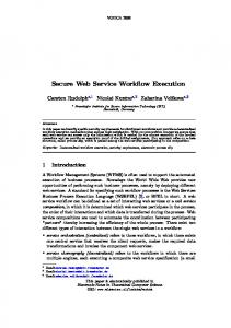
Fig. 2: Extending the two-stage model for different Cloud Providers two, five, ten, twenty five, and a hundred executions on the new cloud. We perform these experiments ten times per cloud provider. Without loss of generality we perform these experiments only for the two-stage approach when using RF, since based on our previous experiments, RF has shown to achieve the best results for the majority of evaluated workflow tasks. For this experiment we will not apply clustering techniques. This is because the executions on the new cloud may form its own cluster, which may not contain enough data to provide accurate predictions. We illustrate here the obtained results for four tasks of the Wien2k workflow. We do not consider the task LapW2Fermi from this workflow due to its short execution time (below 0.7 secs) for which predictions are challenging

to derive for clouds for which no information is available. Figure 2 depicts the obtained results using a Boxplot representation for every cloud provider. The graphs included in that figure illustrate a substantial drop in prediction accuracy (compared to the results reported in Section 6.2) when no data on a given cloud is available. Nevertheless, the obtained predictions are in some cases more accurate than the evaluated related-work based methods as shown in Table 8. If we consider the four evaluated tasks in this section, prediction accuracy ranges between 50% and 14% when no data is available for the new cloud. These results indicate that porting the model to a new provider is a complex issue that may result in low prediction accuracy when no data for the new cloud is available.



On the other hand, the obtained results also show that by performing only a few trial runs on the new provider, the quality of the model quickly improves. In some cases, the RAE falls below 10% with only five task executions on the new provider (see tasks pforLapW1 and Mixer for Amazon EC2 and Rackspace Clouds). Obviously, as depicted by the graph, the more data for the new cloud is included in the training data, the better the resulting prediction accuracy, which tends to converge towards the results reported in Section 6.2. An interesting observation can be made for instance for task pforLapW2 for Amazon EC2 and Rackspace which yields better predictions without data than using a single execution on the new cloud. The reasons for this behavior is the inherent noise of ML methods. With only one execution the model tries to predict for the new cloud, but the data are not enough to generate a suitable model. This effect diminishes when five or more executions in the new cloud are included in the training data.

model. This approach may be sensible for highly dynamic cloud workloads. A possible solution to overcome this problem may require an update of our predictor after every task execution (i.e., retrain the model every time new data is available). This scenario will be a subject to future work. In addition, we will also examine the use of the model proposed in this paper to support different scheduling and resource provisioning techniques.

ACKNOWLEDGMENT This paper has received funding from the European Unions Horizon 2020 research and innovation programme as part of the ENTICE project under grant agreement No 644179.

R EFERENCES [1] [2] [3]

7

C ONCLUSIONS AND F UTURE W ORK

In this paper we have addressed the problem of predicting the execution time of workflow tasks for varying input data for different IaaS clouds. Given a task to be executed on a specific cloud, our method predicts the execution time for different input data in two stages. The first stage predicts the value of the runtime parameters based on historical data for that task on the given cloud or on another cloud. The second stage uses all the predicted runtime parameters together with preruntime parameters to predict the execution time of the task. Experiments for the tasks composing four real workflow applications demonstrate that our two-stage based approach clearly outperforms existing prediction approaches, which are primarily based on pre-runtime parameters. To demonstrate the advantage of our two-stage approach versus a prediction based on pre-runtime parameters, we evaluated the use of different machine learning regression methods such as linear regression, multi-layer perceptron, regression trees, bagging using regression trees, and random forest. The average relative absolute errors over the task of these four workflows show that the two-stage approach achieves better accuracy when using random forest than with other algorithms. We also observed that two types of tasks are harder to predict than others. These types have short execution times (less than one sec.) and/or are bandwidth dependent tasks. In addition, we also demonstrated that our two-stage model can be used to predict task execution times for new IaaS clouds. With only a few executions the model accuracy can be substantially improved. We analyzed this behavior when porting our model to three commercial clouds: Amazon EC2, Google Computing Engine and Rackspace. We showed that the resulting prediction errors with only five task executions on the new cloud can reach an estimation error of less than 10% for some workflow tasks. For increasing training data on the new cloud, the prediction accuracy consistently improves. To build our predictor, we have first collected all the training data and, afterward, we generate the prediction

[4]

[5]

[6]

[7]

[8]

[9]

[10]

[11]

[12]

[13] [14]

J. Qin and T. Fahringer, Scientific Workflow: Programming, Optimization, and Synthesis with ASKALON and AWDL. Springer, 2012. J. Durillo and R. Prodan, “Multi-objective workflow scheduling in amazon ec2,” Cluster Computing, vol. 17, no. 2, pp. 169–189, 2014. L. Breiman, “Random forests,” Machine Learning, vol. 45, no. 1, pp. 5–32, 2001. [Online]. Available: http://dx.doi.org/10.1023/ A%3A1010933404324 K. L. Spafford and J. S. Vetter, “Aspen: A domain specific language for performance modeling,” in Proceedings of the International Conference on High Performance Computing, Networking, Storage and Analysis, ser. SC ’12. Los Alamitos, CA, USA: IEEE Computer Society Press, 2012, pp. 84:1–84:11. [Online]. Available: http://dl.acm.org/citation.cfm?id=2388996.2389110 S. Seneviratne and D. C. Levy, “Task profiling model for load profile prediction,” Future Generation Computer Systems, vol. 27, no. 3, pp. 245–255, 2011. [Online]. Available: http://www. sciencedirect.com/science/article/pii/S0167739X10001743 B.-D. Lee and J. M. Schopf, “Run-time prediction of parallel applications on shared environments,” in Cluster Computing, 2003. Proceedings. 2003 IEEE International Conference on, Dec 2003, pp. 487–491. N. Kapadia, J. Fortes, and C. Brodley, “Predictive applicationperformance modeling in a computational grid environment,” in High Performance Distributed Computing, 1999. Proceedings. The Eighth International Symposium on, 1999, pp. 47–54. H. Li, D. Groep, and L. Wolters, “An evaluation of learning and heuristic techniques for application run time predictions,” in Proceedings of 11 th Annual Conference of the Advance School for Computing and Imaging (ASCI), 2005. T. Miu and P. Missier, “Predicting the execution time of workflow activities based on their input features,” in Proceedings of the 2012 SC Companion: High Performance Computing, Networking Storage and Analysis, ser. SCC ’12. Washington, DC, USA: IEEE Computer Society, 2012, pp. 64–72. [Online]. Available: http://dx.doi.org/10.1109/SC.Companion.2012.21 R. F. da Silva, G. Juve, M. Rynge, E. Deelman, and M. Livny, “Online task resource consumption prediction for scientific workflows,” Parallel Processing Letters, vol. 25, no. 03, p. 1541003, 2015. [Online]. Available: http://www.worldscientific.com/doi/ abs/10.1142/S0129626415410030 A. Matsunaga and J. A. B. Fortes, “On the use of machine learning to predict the time and resources consumed by applications,” in Proceedings of the 2010 10th IEEE/ACM International Conference on Cluster, Cloud and Grid Computing, ser. CCGRID ’10. Washington, DC, USA: IEEE Computer Society, 2010, pp. 495–504. [Online]. Available: http://dx.doi.org/10.1109/CCGRID.2010.98 W. Smith, I. Foster, and V. Taylor, “Predicting application run times with historical information,” J. Parallel Distrib. Comput., vol. 64, no. 9, pp. 1007–1016, Sep. 2004. [Online]. Available: http://dx.doi.org/10.1016/j.jpdc.2004.06.008 P. Dinda, “Online prediction of the running time of tasks,” in High Performance Distributed Computing, 2001. Proceedings. 10th IEEE International Symposium on, 2001, pp. 383–394. P. Dinda and D. O’Hallaron, “An evaluation of linear models for host load prediction,” in High Performance Distributed Computing, 1999. Proceedings. The Eighth International Symposium on, 1999, pp. 87–96.



[15] A. M. Chirkin and S. V. Kovalchuk, “Towards better workflow execution time estimation,” IERI Procedia, vol. 10, pp. 216 – 223, 2014. [Online]. Available: http://www.sciencedirect.com/ science/article/pii/S2212667814001282 [16] I. Pietri, G. Juve, E. Deelman, and R. Sakellariou, “A performance model to estimate execution time of scientific workflows on the cloud,” in Proceedings of the 9th Workshop on Workflows in Support of Large-Scale Science, ser. WORKS ’14. Piscataway, NJ, USA: IEEE Press, 2014, pp. 11–19. [Online]. Available: http://dx.doi.org/10.1109/WORKS.2014.12 ˇ [17] D. A. Monge, M. Holec, F. Zelezn y, ´ and C. Garino, “Ensemble learning of runtime prediction models for gene-expression analysis workflows,” Cluster Computing, vol. 18, no. 4, pp. 1317–1329, 2015. [Online]. Available: http://dx.doi.org/10.1007/ s10586-015-0481-5 [18] S. Lee, J. S. Meredith, and J. S. Vetter, “Compass: A framework for automated performance modeling and prediction,” in Proceedings of the 29th ACM on International Conference on Supercomputing, ser. ICS ’15. New York, NY, USA: ACM, 2015, pp. 405–414. [Online]. Available: http://doi.acm.org/10.1145/2751205.2751220 [19] N. R. Tallent and A. Hoisie, “Palm: Easing the burden of analytical performance modeling,” in Proceedings of the 28th ACM International Conference on Supercomputing, ser. ICS ’14. New York, NY, USA: ACM, 2014, pp. 221–230. [Online]. Available: http://doi.acm.org/10.1145/2597652.2597683 [20] A. Bhattacharyya and T. Hoefler, “Pemogen: Automatic adaptive performance modeling during program runtime,” in Proceedings of the 23rd International Conference on Parallel Architectures and Compilation, ser. PACT ’14. New York, NY, USA: ACM, 2014, pp. 393–404. [Online]. Available: http://doi.acm.org/10.1145/ 2628071.2628100 [21] A. Li, X. Zong, S. Kandula, X. Yang, and M. Zhang, “Cloudprophet: Towards application performance prediction in cloud,” SIGCOMM Comput. Commun. Rev., vol. 41, no. 4, pp. 426–427, Aug. 2011. [Online]. Available: http://doi.acm.org/10. 1145/2043164.2018502 [22] I. H. Witten, E. Frank, and M. A. Hall, Data Mining: Practical Machine Learning Tools and Techniques, 3rd ed. San Francisco, CA, USA: Morgan Kaufmann Publishers Inc., 2011. [23] S. Salzberg, “C4.5: Programs for machine learning by j. ross quinlan. morgan kaufmann publishers, inc., 1993,” Machine Learning, vol. 16, no. 3, pp. 235–240, 1994. [Online]. Available: http://dx.doi.org/10.1007/BF00993309 [24] J. W. Shavlik, R. J. Mooney, and G. G. Towell, “Symbolic and neural learning algorithms: An experimental comparison,” Machine learning, vol. 6, no. 2, pp. 111–143, 1991. [25] T. M. Mitchell, Machine Learning, 1st ed. New York, NY, USA: McGraw-Hill, Inc., 1997. [26] H. Trevor, T. Robert, and F. Jerome, The Elements of Statistical Learning, 2nd ed. Springer, 2009. [27] L. Breiman, “Bagging predictors,” Machine Learning, vol. 24, no. 2, pp. 123–140, 1996. [Online]. Available: http://dx.doi.org/ 10.1007/BF00058655 [28] T. G. Dietterich, “Ensemble methods in machine learning,” in Proceedings of the First International Workshop on Multiple Classifier Systems, ser. MCS ’00. London, UK, UK: Springer-Verlag, 2000, pp. 1–15. [Online]. Available: http://dl.acm.org/citation.cfm?id= 648054.743935 [29] J. C. Jacob, D. S. Katz, G. B. Berriman, J. C. Good, A. C. Laity, E. Deelman, C. Kesselman, G. Singh, M. Su, T. A. Prince, and R. Williams, “Montage: a grid portal and software toolkit for science;grade astronomical image mosaicking,” Int. J. Comput. Sci. Eng., vol. 4, no. 2, pp. 73–87, Jul. 2009. [Online]. Available: http://dx.doi.org/10.1504/IJCSE.2009.026999 [30] P. Blaha, K. Schwarz, G. Madsen, D. Kvasnicka, and J. Luitz, “Wien2k,” An augmented plane wave+ local orbitals program for calculating crystal properties, 2001. [31] P. T., “Povray - persistence of vision parallel raytracer,” in Proceedings of Computer Graphics International Conference, ser. CGI ’98, 1998, pp. 123–129. [32] S. Loew, “Rendering blender on the grid, Master Thesis, University of Innsbruck,” 2008. [33] I. Guyon and A. Elisseeff, “An introduction to variable and feature selection,” Journal of machine learning research, vol. 3, no. Mar, pp. 1157–1182, 2003. [34] T. Fahringer, R. Prodan, R. Duan, F. Nerieri, S. Podlipnig, J. Qin, M. Siddiqui, H.-L. Truong, A. Villazon, and M. Wieczorek,

“Askalon: A grid application development and computing environment,” in Proceedings of the 6th IEEE/ACM International Workshop on Grid Computing, ser. GRID ’05. Washington, DC, USA: IEEE Computer Society, 2005, pp. 122–131. [Online]. Available: http://dx.doi.org/10.1109/GRID.2005.1542733 [35] J. S. Armstrong and F. Collopy, “Error measures for generalizing about forecasting methods: Empirical comparisons,” International Journal of Forecasting, vol. 8, pp. 69–80, 1992. [36] M. Ester, H.-P. Kriegel, J. Sander, and X. Xu, “A density-based algorithm for discovering clusters in large spatial databases with noise.” AAAI Press, 1996, pp. 226–231. [37] A. P. Dempster, N. M. Laird, and D. B. Rubin, “Maximum likelihood from incomplete data via the em algorithm,” JOURNAL OF THE ROYAL STATISTICAL SOCIETY, SERIES B, vol. 39, no. 1, pp. 1–38, 1977.

Thanh-Phuong Pham received the Master degree at faculty of computer science and engineering, University of Technology, Vietnam in 2011. He received the second master in computer science from University of Nice Sophia Antipolis, France, in 2012. He is currently PhD student in the Distributed and Parallel Systems Group at the University of Innsbruck, Austria. His research interests include fault tolerance, machine learning, data analysis and performance prediction for distributed computing.

Juan J. Durillo received PhD in Computer Science from the University of Mlaga ,Spain in 2011. Currently, he is an assistant professor in the Distributed and Parallel Systems Group at the University of Innsbruck, Austria. His main research interests are Single and Multi-criterion Optimization , Parallel and Distributed Computing , Cloud Computing, Software Auto-tuning,Search Based Software Engineering, Green Computing, GPU Computing

Thomas Fahringer received his PhD degree from the Vienna University of Technology in 1993. Since 2003, he has been a full professor of computer science at the Institute of Computer Science, University of Innsbruck, Austria. His main research interests include software architectures, programming paradigms, compiler technology, performance analysis, and prediction for parallel and distributed systems. He is a member of the IEEE.


Predicting Workflow Task Execution Time in the Cloud using A Two

Predicting Workflow Task Execution Time in the Cloud using A Two

Suggest Documents

Predicting Task Execution Time on Handheld Devices Using the ...

Predicting the Execution Time of Grid Workflow ... - Semantic Scholar

Towards Better Workflow Execution Time Estimation - ScienceDirect

Estimating the Execution Time Distribution for a Task ... - CiteSeerX

Fault-Tolerant BPEL Workflow Execution via Cloud ... - Semantic Scholar

A Retargetable Technique for Predicting Execution Time - Computer

A Workflow Approach towards GLIF Execution

Secure Web Service Workflow Execution

Contextualised Workflow Execution in MyGrid - CiteSeerX

Execution Time Estimation for Workflow Scheduling - Semantic Scholar

Execution Time Estimation for Workflow Scheduling 1 ...

Contextualised Workflow Execution in MyGrid - Semantic Scholar

Optimal Workflow Execution in Grid Environments

In-Execution Malware Detection using Task Structures of Linux ...

In-Execution Malware Detection using Task Structures of ... - CiteSeerX

Enhancing the flexibility of workflow execution by

Task Balanced Workflow Scheduling Technique considering Task ...

Software Execution Protection in the Cloud - CiteSeerX

Predicting detection task performance using a visual ...

Interactive Execution Time Predictions using Reference ... - CiteSeerX

Static Worst-Case Execution Time Optimization using

Visualizing Parallel Execution Traces using Logical Time

Predicting Query Execution Time: Are Optimizer Cost ... - CiteSeerX

Robust Scheduling of Task Graphs under Execution Time Uncertainty